Determination of Monitoring Control Value for Concrete Gravity Dam Spatial Deformation Based on POT Model

1  Introduction

To ensure the safety operation of dams, it is necessary to understand the service behavior of dams by analyzing monitoring data in real time [1–5]. Dam deformation is one of the main means to monitor and judge the operation behavior of the dam. The deformation monitoring control value is a crucial index to evaluate and monitor dam safety. If the control value is too large, the danger cannot be found in time. If the control value is too small, it tends to be conservative. Therefore, the determination of appropriate monitoring control value is pivotal for evaluating the service safety of the dam.

The commonly used methods to estimate the control value of monitoring effect quantity are mathematical statistics and structural analysis. For the long-term monitoring data series, mathematical statistics is usually used to formulate the control value of dam deformation monitoring effect quantity. Yang et al. [6] proposed an expression of temperature entropy in concrete dams based on the synergetics and entropy, and determined the sequential value and the early-warning index value of temperature entropy with this expression via the small probability method. Lei et al. [7] established an entropy formula to measure the deformation of high concrete dam, and suggested a method of calculating early warning index of spatial deformation by low probability principle based on series of calculated deformation entropy values. Qin et al. [8] presented a multi-block combined diagnosis indexes based on dam block comprehensive displacement of concrete dams, which is made up of single-point displacements with different weights determined with improved projection pursuit method (PPM). Su et al. [9] extracted inherent characteristics of deformation and seepage accurately using the kernel principal component analysis (KPCA) method and determined the spatial multi-point security warning domain of deformation and seepage in typical dam sections. Li et al. [10] proposed an online robust recognition and early warning model based on an M-estimator and a confidence interval, and a threshold 3ST+D is set by the scale estimator ST based on the location M-estimator and the derived confidence interval calculation formula D based on the robust regression. Chen et al. [11] constructed a new early warning index of dam deformation using the forward-simulated deformation and other components of the statistical model. Chen et al. [12] proposed a novel dynamic early-warning model using deep learning and spatiotemporal features fusion for dam deformation, and determined early-warning indicator using cloud synthesis. Su et al. [13] presented the early-warning index of structural response under the load combinations by analyzing the capacity bearing the past loads and estimating the capacity bearing the future possible loads for one dam body-foundation system. Yang et al. [14] proposed a method for determining multistage warning indicators for the overall deformation of concrete dam considering fuzziness and randomness. Wang et al. [15] examined safety monitoring index of high concrete gravity dam based on failure mechanism of instability, and the progressive instability failures of concrete gravity dams under various failure modes were investigated with the FEM combined with strength reduction and overloading methods. Li et al. [16] proposed 12 key evaluation indexes of a dynamic early warning system to efficiently predict an early dam break signal for a tailings dam based on the dynamic grey relation analysis method.

Many monitoring points are often arranged for dam monitoring, but the traditional dam monitoring control values are mostly based on a single monitoring point on deformation, seepage or stress, ignoring the spatial correlation between the monitoring points. Fully considering the correlation characteristics of time and space distribution of monitoring information at multiple measuring points, comprehensively reflecting the integrity of dam deformation can more effectively reflect the overall working behavior of the dam. In this study, the plane deformation field of the positive inverted vertical line measuring points in the concrete gravity dam is constructed. The projection pursuit method (PPM) [17] combined with the grey wolf optimization (GWO) algorithm [18] is used to project the deformation field data to the low dimensional space, and the peaks over threshold (POT) model [19] is used to comprehensively determine the threshold value. The POT model is improved with the automatic threshold determination method based on the 3σ criterion in probability theory and the GWO algorithm, which can avoid the subjectivity and randomness for determining the threshold. In addition, the proposed method is applied to Wuqiangxi concrete gravity dam to verify its feasibility.

The rest of the manuscript is structured as follows. The methodology is described in Section 2. Case studies and discussion are given in Section 3. Some conclusions are presented in Section 4.

2  Methodology

The traditional dam monitoring control values are determined based on the measured values of single measuring point, ignoring the spatial correlation among measuring points. In this work, the deformation field is constructed according to the characteristics of the measuring points of the positive inverted vertical lines. The PPM combined with the GWO algorithm is used to project the deformation field data into the low dimensional space, and the comprehensive displacement of the dam deformation is determined according to the weight of each measuring point. The POT model is improved by using automatic threshold determination method, which evaluates the threshold based on the 3σ criterion in probability theory and the GWO algorithm. Using the improved POT model, the monitoring control values of the dam deformation field are determined with the obtained comprehensive displacement of the dam deformation.

2.1 Dam Comprehensive Deformation Displacement

A large number of monitoring instruments are arranged at different parts of the dam to jointly monitor the working behavior of the dam. In fact, the deformation of each measuring point is not independent. The correlation of the spatial structure exists. Therefore, it is necessary to comprehensively consider the correlation among spatial monitoring effects, and mine the spatial characteristics and development laws of dam deformation from the data.

With the development of spatial metrology, data representation methods have been expanded from one dimension to a high dimension, from time or cross-section to spatial panel data, and combination of cross-section, time and spatial data. For the dam, the deformation data of each measuring point is not independent of each other, but there is spatial structure correlation under the action of external load. Therefore, it is necessary to comprehensively consider the correlation between different spatial monitoring effects, and mine the spatial characteristics and development laws of dam deformation from the data.

The horizontal displacement vector field δ generated by concrete dam under external load can be decomposed into horizontal along river displacement δu and horizontal across river displacement δv, i.e.,

δ=δu(x,y,z)i+δv(x,y,z)j(1)

where i and j are the unit vectors along the river and across the river, respectively.

The monitoring values of all measuring points at the same time of the dam can generally reflect the spatial deformation behavior of the structural system. For the vertical measuring points of the typical dam section of a concrete gravity dam, by continuously monitoring the downstream or transverse deformation of all measuring points on a vertical line, the downstream or transverse deformation values of different elevations at different times can be obtained as follows:

δ=[δ11⋯δ1T⋮⋮⋮δn1⋯δnT](2)

where n denotes the number of elevations, and T is the number of times.

δ contains the deformation information of different parts of the dam body, so it can fully reflect the dynamic changes of the dam deformation field. The measured values of spatial deformation sequence are transformed into comprehensive deformation δj′ by PPM as follows:

δj′=wiδij(3)

where wi denotes the weight value of the measuring point of ith elevation.

2.2 Determination of Weight Values of Measuring Points Based on PPM-GWO

The information contained in the spatial deformation section data of the dam is mined with the PPM, then the weight distribution of each measuring point at different elevations of a certain section of the dam can be determined. The PPM searches the projection direction that can comprehensively reflect the characteristics or structure of the original high-dimensional data by polarizing a projection index, projects the high-dimensional data to the low-dimensional subspace, and analyzes the high-dimensional data by studying the data structure and projection characteristics of the low-dimensional space.

The samples of all displacement measuring points can be expressed as {δij|i=1,2,...,n;j=1,2,...,p}, n is the number of samples, and p is the number of indexes in the sample. δij is the jth measured value of the ith elevation measuring point. δij is normalized as δ¯ij.

δ¯ij=δij−δiminδimax−δimin(4)

where δimax and δimin are the maximum value and minimum value in the measured value sequence of the ith elevation measuring point, respectively.

Normalized measured value sequence {δ¯ij|i=1,2,...,n;j=1,2,...,p} is integrated into a comprehensive projection value with l=(l1,l2,...,lp) as the projection direction.

Ti=∑j=1pliδ¯ij(5)

where ∑i=1nli2=1.

After the normalized sample set is determined, the value of the projection index function Z(l) will be determined by the projection direction l and will change accordingly. According to the relationship between l and Z(l), the maximum value of Z(l) corresponds to the best projection direction l∗. The objective function h(l) of the problem is expressed as

maxh(l)=STZT(6)

with

ST=1n−1∑i=1n[T(i)−T¯(i)]2(7a)

ZT=∑i=1n∑j=1p(R−rij)f(R−rij)(7b)

where ST and ZT are the divergence of projection value and projection index function, respectively; T¯(i) is the average value of data sequence T(i); R=0.1ST is the window radius of local density; Rij is the distance between projected values; f(t) is the unit step function, which satisfies f(t) = 1(t ≥ 0) and f(t) = 0(t < 0).

The GWO algorithm is a global random search algorithm established by simulating the hunting and search behavior of grey wolves in the process of hunting. The GWO algorithm is similar to the particle swarm optimization (PSO). It is a random search algorithm that converges to the global optimal solution with a large probability. Compared with the PSO, grid search optimization algorithm, the GWO has fewer parameters, simple structure and strong convergence. In this study, the GWO algorithm is used to solve the objective function of the PPM to determine the weight of spatial measurement points.

The best, second and third best solutions are respectively considered as α, β and δ, and other solution is assumed to be ω. In the GWO algorithm, hunting (optimization) is guided by α, β and δ, and ω wolves follow them. In the process of hunting, vector of the grey wolf’s positions X is updated by [18]

X(t+1)=Xp(t)−A⋅D(8)

with

D=|C⋅Xp(t)−X(t)|(9a)

A=2a⋅r1−a(9b)

C=2r2(9c)

where t denotes the number of iterations, Xp(t) is the vector of prey’s positions, a is the vector set to decrease linearly from 2 to 0 over the iterations, and r1 and r2 are the random vectors in [0,1].

To simulate the hunting behavior of grey wolves, α (best candidate for the solution), β, and δ are assumed to have more knowledge about the potential position of the prey. The algorithm saves three best solutions achieved so far and forces others (i.e., ω wolves) to update their positions to achieve the best place in the decision space. In the optimization algorithm, such a hunting behavior can be modeled by [18]

X1(t+1)=Xα(t)−A1⋅Dα(10a)

X2(t+1)=Xβ(t)−A2⋅Dβ(10b)

X3(t+1)=Xδ(t)−A3⋅Dδ(10c)

with

Dα=|C1⋅Xα(t)−X(t)|(11a)

Dβ=|C2⋅Xβ(t)−X(t)|(11b)

Dδ=|C3⋅Xδ(t)−X(t)|(11c)

where Xα(t), Xβ(t) and Xδ(t) are the present positions of α, β and δ, respectively; C1, C2 and C3 are the random vectors.

The main procedures of the GWO algorithm are as follows: (1) Utilize initial parameters (number of grey wolves, number of iterations, etc.); (2) Create initial population of grey wolves with different social hierarchy (α, β, δ and ω); (3) Estimate the prey’s positions by α, β and δ; (4) Estimate the positions of the grey wolves by the prey’s positions; (5) Grade the grey wolves; (6) End when stopping criteria is satisfied, otherwise go to (3).

Mark the obtained best projection direction as l∗, and the projection values of the sample points can be obtained withEq. (5). Then, the weight value of each measuring point is calculated with

wi=T∗(i)∑i=1nT∗(i)(12)

where T∗(i) is the best projection value of the measured value of the ith measuring point.

2.3 Determination of Monitoring Control Values Based on POT Model

The POT model in extreme value theory focuses on the sequence distribution beyond the threshold, which can better consider the occurrence of large measured values, and the calculated results are more close to the actual situation of dam operation and service.

For the comprehensive displacement {x1,x2,...,xn} of the dam deformation field, let its distribution function be F(x), the threshold value is m, and nm is the number of values exceeding the threshold in the sequence {x1,x2,...,xn}. When the dam displacement xi is greater than the threshold value m, the displacement greater than the threshold value is yi, i.e., yi=xi−m (yi≥0). The conditional distribution function of {y1,y2,...,yt} (t < n) can be obtained with [19]

Fm(y)=P(x−m≤y|x>m)=F(x)−F(m)1−F(m)(13)

According to the extreme value theorem, when the threshold is large enough, it converges to the generalized Pareto distribution.

Fm(y)≈Gξ,σ(y)={1−(1+ξσy)−1ξξ≠01−e−yσξ=0(14)

where σ is the scale parameter, ξ is the shape parameter, y∈[0,∞) for ξ≥0, and y∈[0,−σξ] for ξ<0.

As long as the threshold value is determined, the transfinite sequence can be obtained. The shape parameter and scale parameter can be solved by using the maximum likelihood function, which is expressed as

L(ξ,σ|y)={−nlnσ−(1+1ξ)∑i=1nln(1+ξσyi)ξ≠0−nlnσ−1σ∑i=1nyiξ=0(15)

After ξ and σ are known, the over threshold distribution function F(y) can be determined, so that the monitoring control value of F−1(x) under a certain quantile can be solved. The probability function of abnormal dam deformation is

P(x<xα)=Pα=∫xα∞f(x)dx(16)

where xα is the extreme value or warning value of dam displacement monitoring under different probabilities α, Pα is probability, and f(x) is the probability density.

Thus, the estimated value of xα is obtained as follows:

x^α={u+σξ(nnmPα−1)ξ≠0u−σln(nnmPα)ξ=0(17)

In the process of using the POT model to draw up dam displacement monitoring control values, if the threshold value is too large, the variance of estimated values of shape and scale parameters will be too large due to too few samples exceeding the limit value; If the threshold value is too small, the distribution of the over limit value may not converge, resulting in great errors for determining monitoring control values. The methods to determine the threshold value mainly include over limit expectation graph method and Hill graph method. Both of these two methods are graphical methods, which are more intuitive, but require manual judgment, which is easy to cause subjective errors. In this paper, 3σ criterion is used as the theoretical basis to construct the function to determine the threshold, and the GWO algorithm is used to find the optimal threshold.

According to the 3σ criterion in probability, set the mean and standard deviation of the sample as μ and σ. When the number of measurements is large enough, the probability of value interval distribution is as follows: (1) the probability is 0.6826 for [μ−σ,μ+σ]; (2) the probability is 0.9545 for [μ−2σ,μ+2σ]; (3) the probability is 0.9973 for [μ−3σ,μ+3σ]. It is considered that the probabilities of the measured value which is located in [μ−3σ,μ+3σ] and [μ−2σ,μ+2σ] are 0.27% and 4.55%, respectively. Then, ±3σ is used to determine the dangerous value x0.27% in the effect quantity monitoring control value, and ±2σ is used to determine the early warning value x4.55% in the effect quantity monitoring control value. It can be concluded that the difference between the danger value and the early warning value is about the standard deviation of the sample, i.e, Δ=|x0.27%−x4.55%|=σ.

The steps of threshold selection based on the GWO algorithm are as follows: (1) Determine the upper and lower limits of the threshold. The threshold sequence meets the convergence of the conditional distribution function Fm(y) and the generalized Pareto distribution of the transfinite sequence corresponding to the threshold, and the upper and lower limits of the threshold that meet the conditions shall be selected according to the weighted comprehensive displacement. (2) Construct the threshold matrix. According to the upper and lower threshold values, a n × p threshold matrix is established. Each row has p random numbers between the upper and lower threshold values, that is, the threshold matrix is {mij|i=1,2,...,n;j=1,2,...,p}. (3) Calculate the monitoring control values of different thresholds. The early warning value xmij,0.455 and danger value xmij,0.027 of the threshold with probability of 0.455 and 0.027 are calculated, respectively. (4) Construct the fitness function. Δij is calculated. The fitness function of GWO algorithm is expressed as min c=|δ−σ|. (5) Calculate the optimal threshold. The optimal threshold in each line of threshold sequence is found using the GWO algorithm according to the fitness function, and the average value is taken as the optimal threshold.

Fig. 1 shows the workflow of determining the monitoring control value for concrete gravity dam spatial deformation based on POT model.

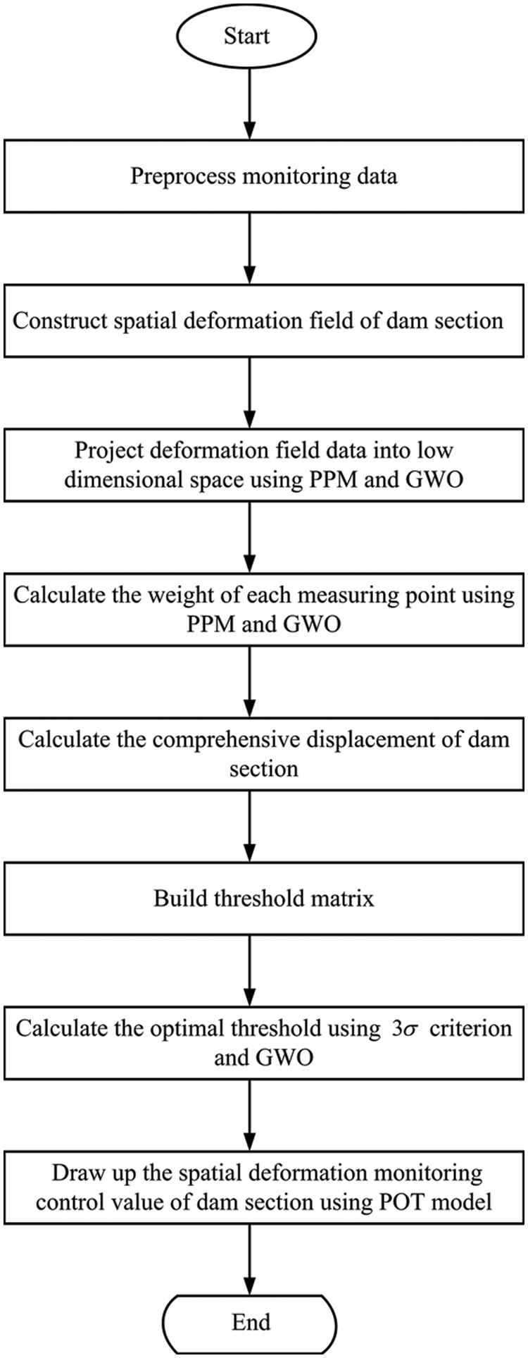
Figure 1: Workflow of determining the monitoring control value for concrete gravity dam spatial deformation based on POT model

3  Case Study and Discussion

3.1 Project Overreview

Fig. 2 presents the location of Wuqiangxi hydropower station, which consists of the river blocking dam, the powerhouse behind the dam and the three-stage ship lock. The schematic diagram of layout of Wuqiangxi hydropower station is shown in Fig. 3. The dam is a concrete gravity dam. The crest elevation is 117.5 m, the highest dam height is 85.83 m, and the total crest length is 719.7 m. The main dam is divided into 33 dam sections, and the layout of dam deformation measuring points is shown in Fig.4.

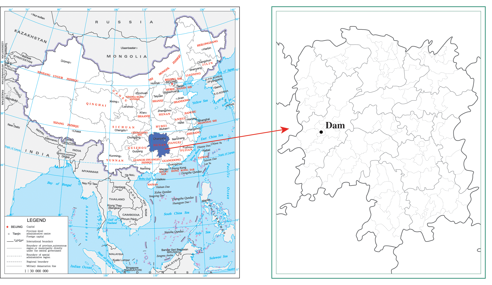
Figure 2: Location of Wuqiangxi hydropower station (the longitude and latitude of the dam are 110.6294 and 28.5783, respectively)

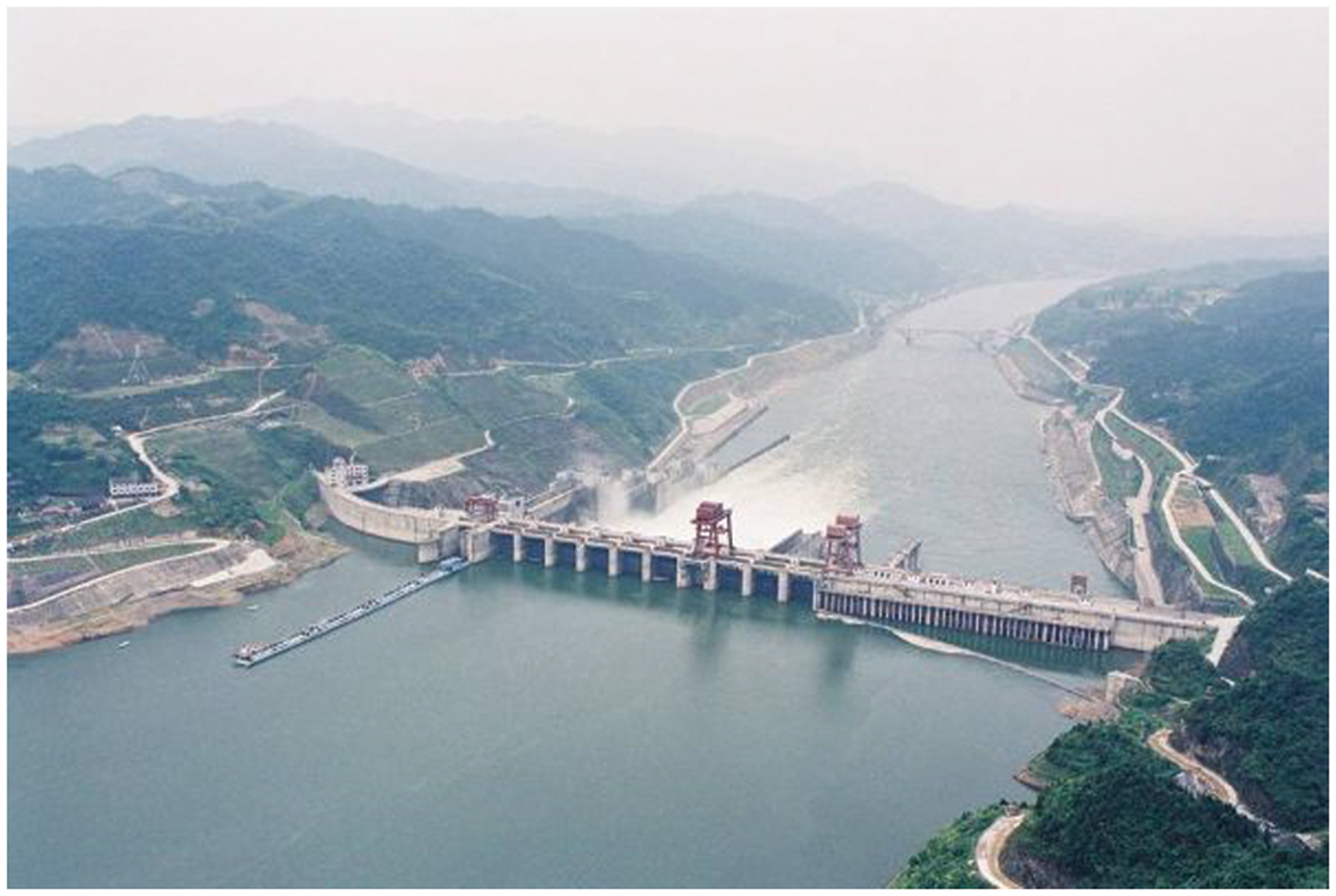
Figure 3: Wuqiangxi hydropower station

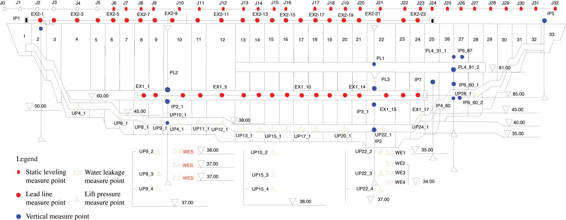
Figure 4: Layout of deformation measuring points

The displacements along the river from January 2011 to December 2020 of the positive inverted vertical lines PL1, PL3, IP3_60 and IP3_39 of dam section 22 (the elevations are 117.5, 81, 61 and 40.2 m, respectively) are taken as the data sample. The gross error is excluded, and the process lines of measured displacements are shown in Fig. 5. The displacement towards the downstream is positive, and the displacement towards the upstream is negative.

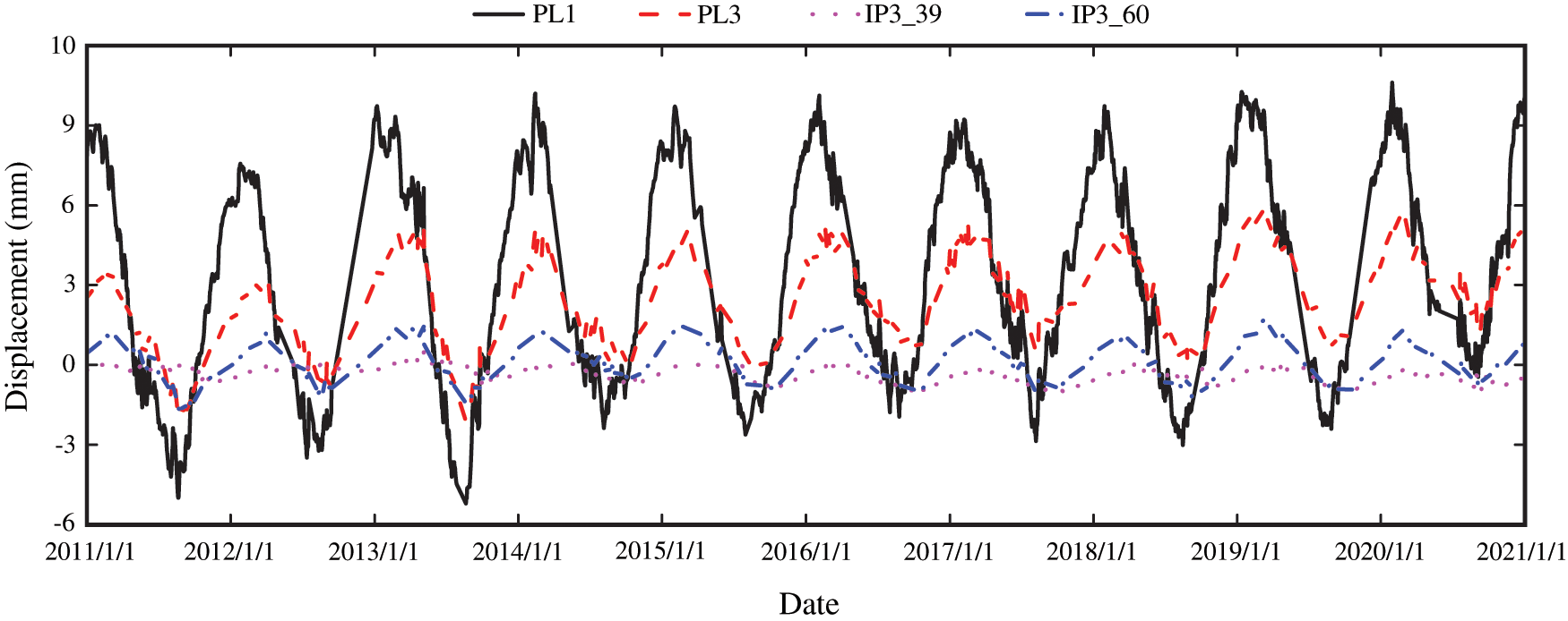
Figure 5: The process lines of measured displacements along the river of all measuring points on dam section 22

3.2 Comparison of Optimization Algorithm Selection

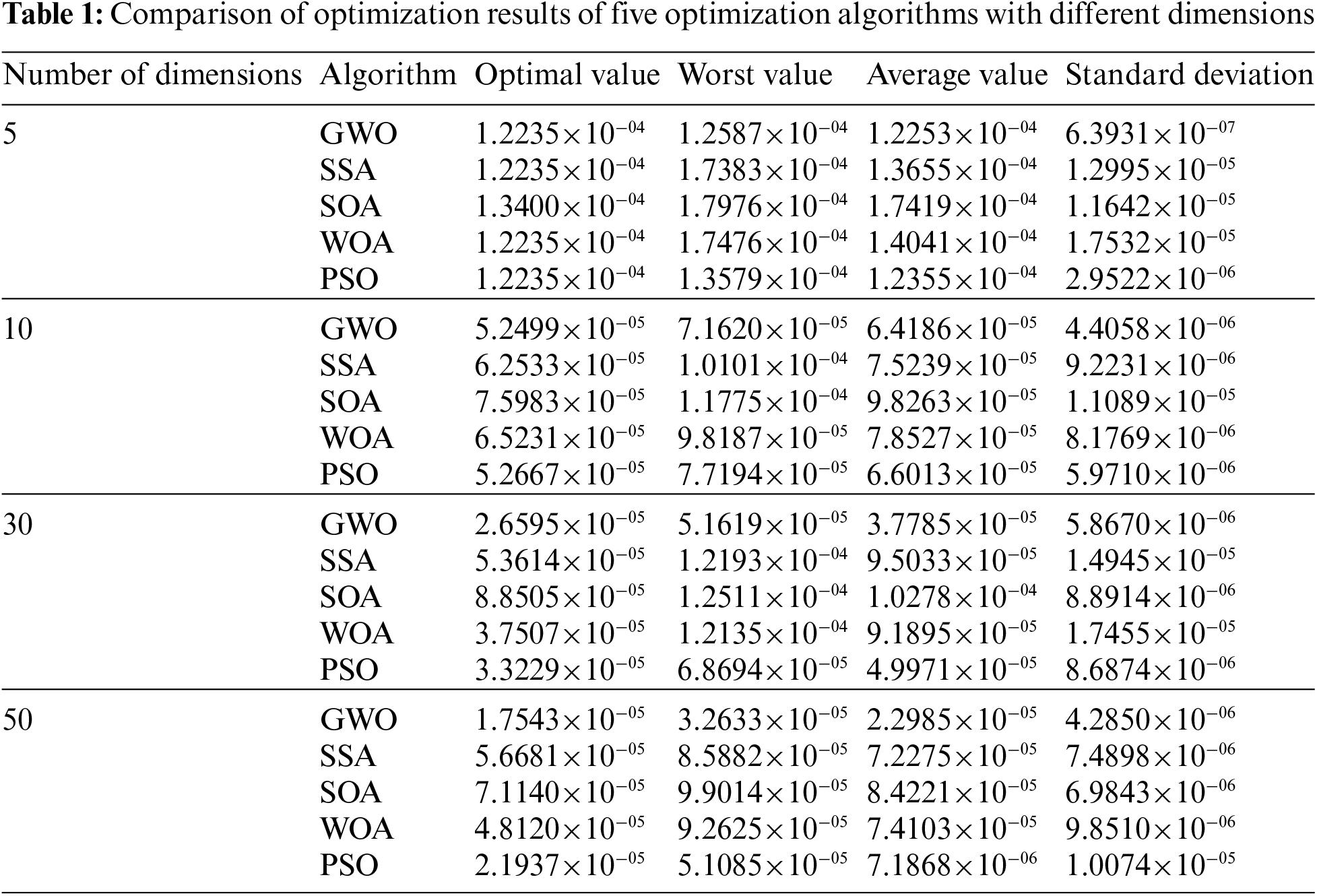
For the PPM to determine the weight of spatial measurement points, we select the sparrow search algorithm (SSA) [20], seagull optimization algorithm (SOA) [21], whale optimization algorithm (WOA) [22] and particle swarm optimization (PSO) algorithm [23] to compare with the GWO algorithm. The function of adjusting the PPM to find the best projection direction changes from finding the maximum value to finding the minimum value. If the upper and lower limits of the test data set are set to [−50, 50], the solution domain is [0.01, 1], the population number is 30, and the maximum number of iterations is 500. For data of different dimensions, each algorithm is solved 30 times independently, and four statistical indicators such as the optimal value, the worst value, the average value and the standard deviation of the fitness are selected to comprehensively evaluate the algorithm.

The variations of fitness values for different algorithms are shown in Fig. 6.

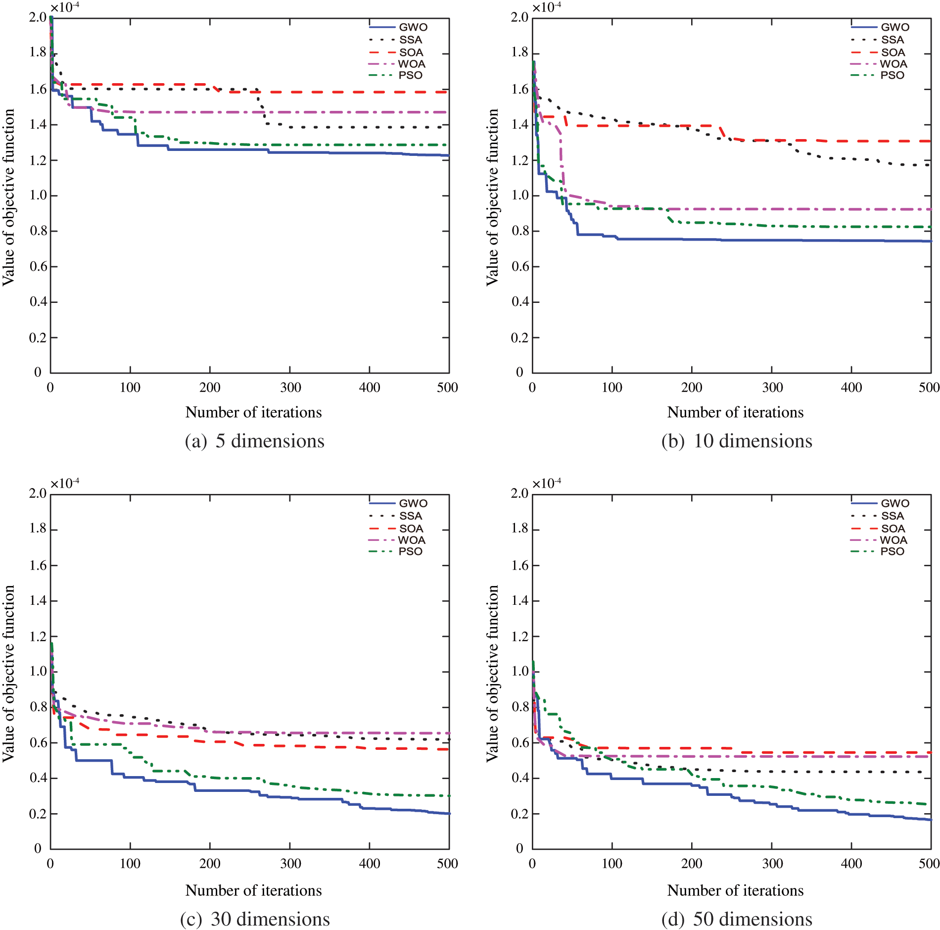
Figure 6: The iteration process of different algorithms

FromTable 1, when the data dimension is low, there is little difference in the optimal values of the fitness of five algorithms, but the worst value and mean value of the GWO’s fitness are the smallest, and the standard deviation of the GWO’s fitness is much smaller than that of the other four algorithms, indicating that the GWO is more stable. With the increase of data dimension, the GWO’s advantages in dealing with the problem of determining the weight of spatial measurement points by PPM are reflected. The optimal value, the worst value, the average value and the standard deviation of the GWO’s fitness are the smallest of the five algorithms, and the higher the dimension, the more obvious the advantages of the GWO. From the iteration curves, it can be found that the GWO algorithm has the best effect. Whether it is high-dimensional or low-dimensional, the GWO has the fastest convergence speed and the highest convergence accuracy at the same iteration times. In conclusion, the GWO has the best effect in dealing with the problem of determining the weight of spatial measurement points by PPM.

3.3 Determination of Measuring Point Weight

The environmental variables have a non-linear relationship with the measuring points at different elevations on the vertical line. In the weighted displacement calculation, the weight should change with the change of environmental quantities, not a fixed value. The environmental quantities in the same month have little difference. Therefore, the data in different months are projected separately. The PPM is used to reduce the dimension of the data of the dam deformation field, and the best projection direction is shown inTable 2. The weight of measuring points in different months is shown in Table 3. According to the weights and data of each measuring point, the comprehensive displacement of the dam section can be obtained, and the process line is shown in Fig.7.

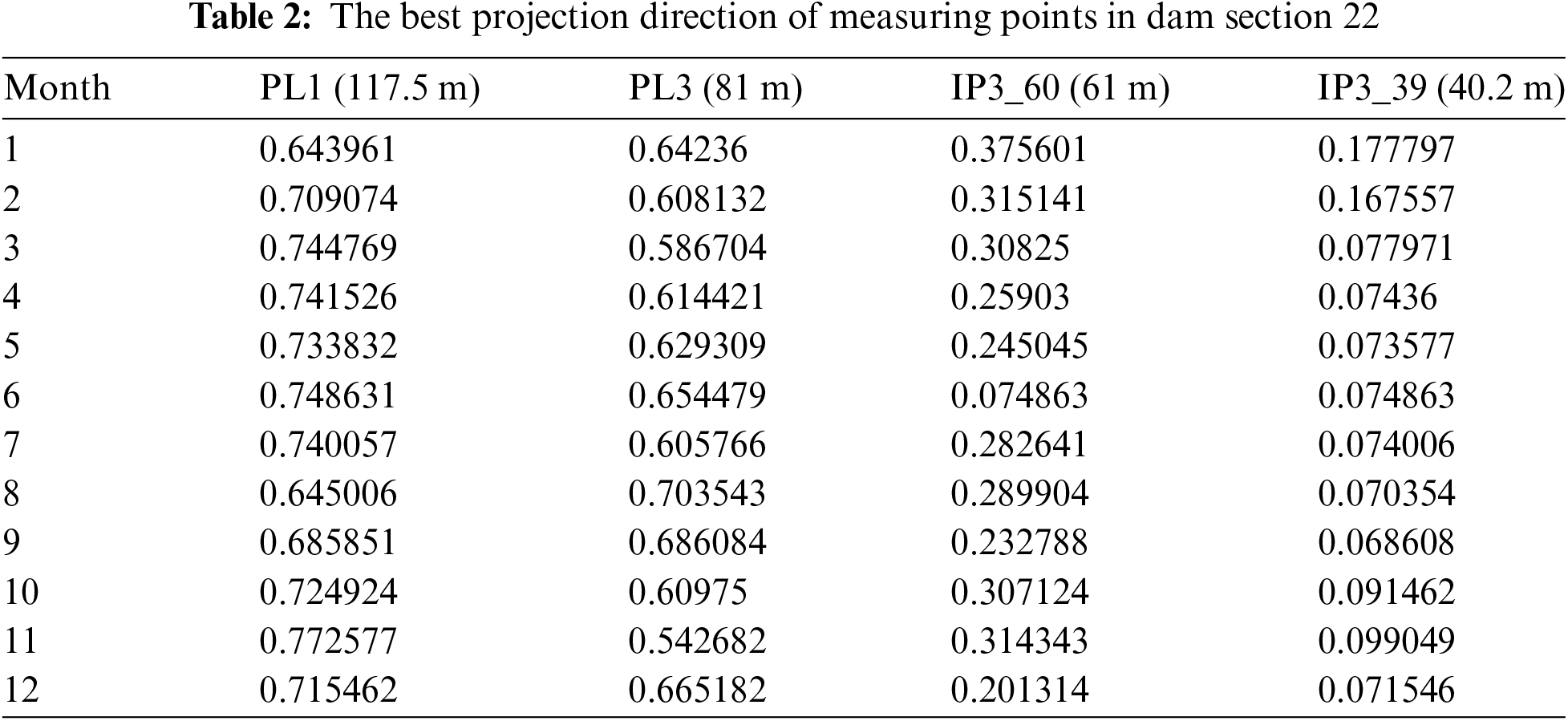
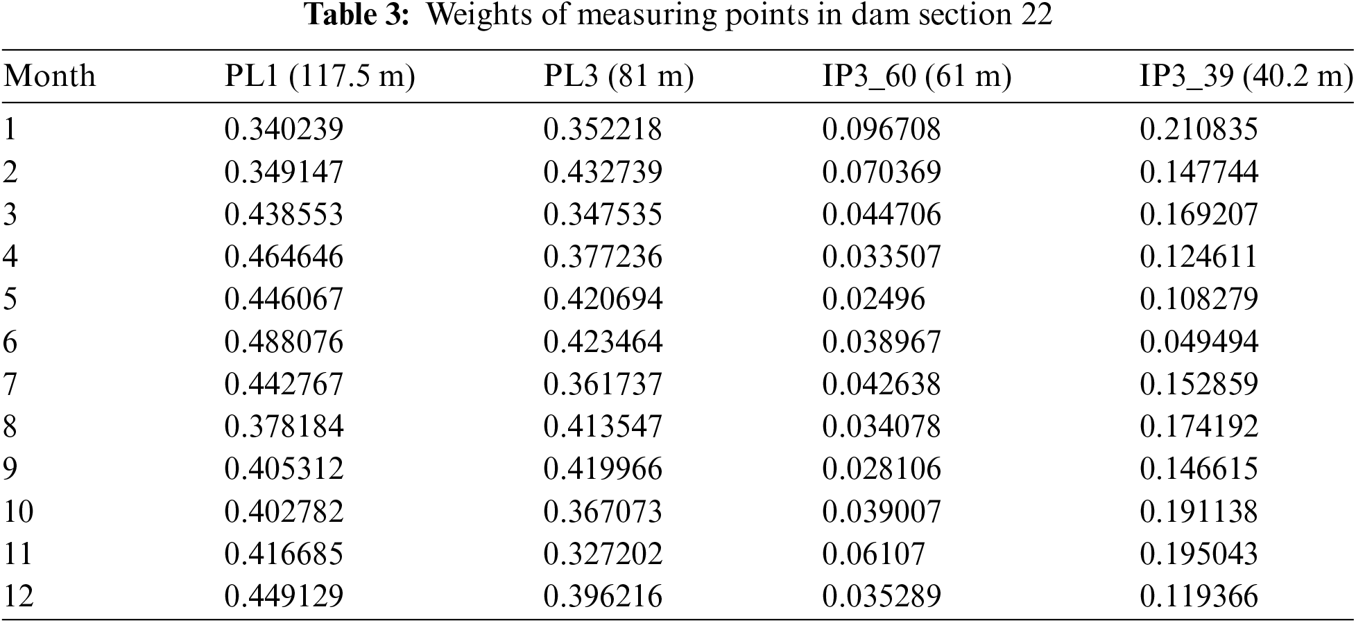
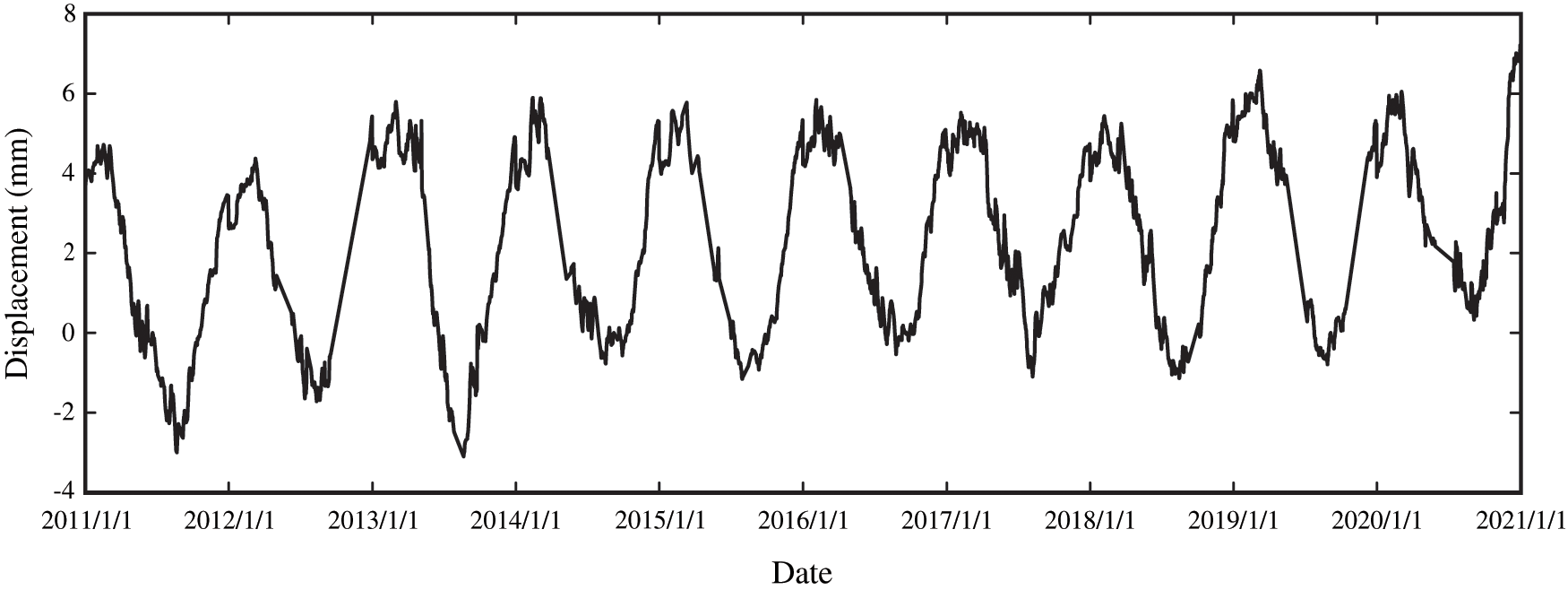
Figure 7: The process line of comprehensive displacement of dam section 22

The obtained comprehensive displacement value integrates the monitoring data of the positive inverted vertical lines of the dam section, and well reflects the variation law of the displacement along the river of the whole dam section. The Q-Q diagram method is used to carry out the heavy-tail test of the downstream displacement data. The results are shown in Fig. 8. It can be seen that the lower end is upward and the upper end is downward on both sides of the diagonal of the comprehensive displacement data, and the middle is approximately in a straight line, which conforms to the characteristics of the heavy-tail distribution of the data and meets the preconditions of the POT model.

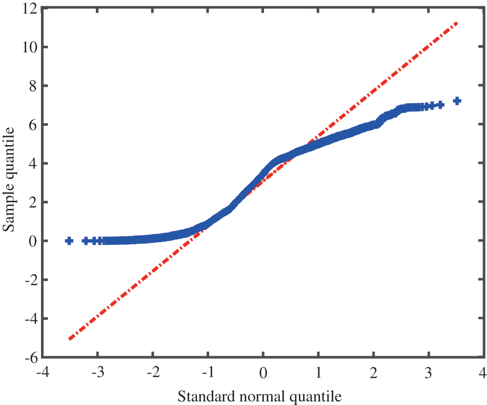
Figure 8: Q-Q diagram of dam section 22

3.4 Determination of Threshold

When determining the threshold, too many or too few tail samples will lead to failure to grasp the characteristics of the tail distribution of the sequence. Generally, it is considered that when the number of tail samples is 10%∼30% of the total samples, the conditional distribution function corresponding to the over threshold sequence converges to the generalized Pareto distribution. Therefore, this paper selects the threshold optimization solution domain as the value corresponding to 30% of the sample data and the value corresponding to the upper limit of 5%, sets the dimension number as 4, and uses the GWO to find the optimal threshold. The transfinite threshold diagram and Hill diagram are drawn according to the downstream displacement data, as shown in Figs. 9 and 10.

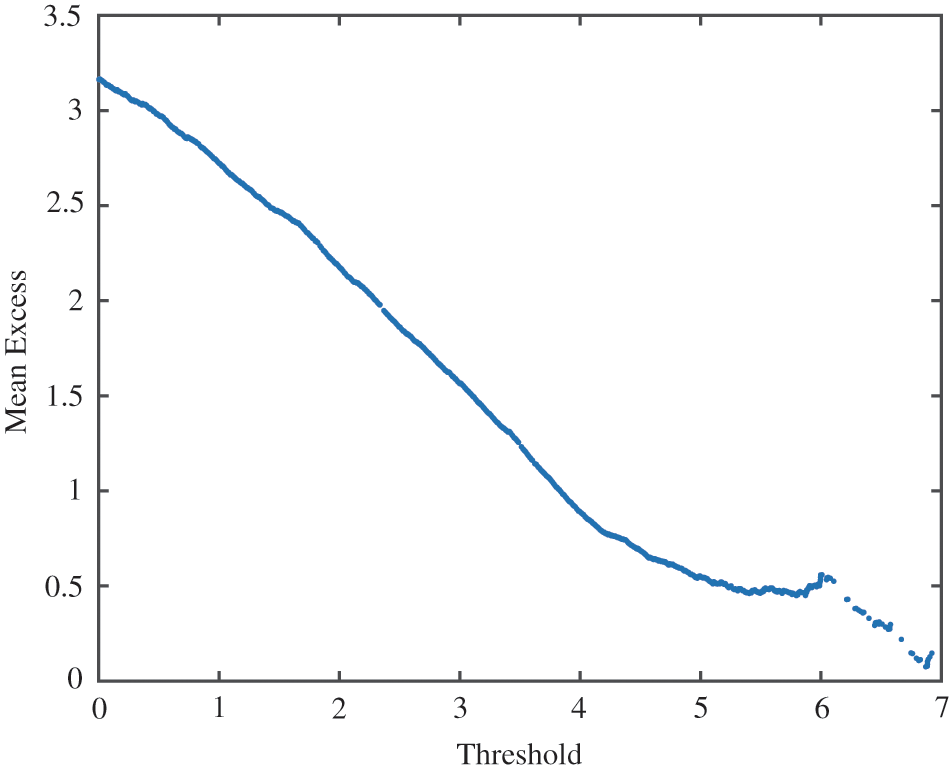
Figure 9: The transfinite threshold diagram of dam section 22

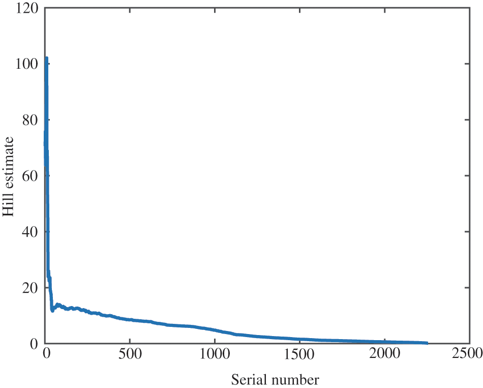
Figure 10: The Hill diagram of dam section 22

The threshold is 5.2886 for the GWO, 5.3 for the transfinite expectation graph, and 5.242 for the Hill diagram. It can be found that the threshold value determined by the threshold value selection method based on the GWO is basically close to the threshold values determined by the transfinite threshold diagram and Hill diagram, which shows that the threshold value selection method based on the GWO is reasonable. After the threshold range is determined, the method automatically finds the optimal threshold value by the GWO. The selected threshold value is more objective and more accurate.

3.5 Determination of Deformation Monitoring Control Value

Taking the probability of 4.55% and 0.27% as the probability of early warning value and danger value, the monitoring index of downstream displacement, the parameters and calculation results of the POT model based on the GWO to determine the threshold are as follows: the number of samples is 2285, the number of over threshold is 2254, the shape parameter is −0.12361, the scale parameter is 0.54055, the early warning value is 7.7416 mm, and the danger value is 9.5338 mm.

In this paper, the cloud model (CM) [24] is used to test the calculation results. The CM model is a model based on the principle of normal distribution. The reverse cloud generator is used to calculate the expectation Ex, entropy En and super entropy He of the weighted displacement value of the dam. The positive cloud generator is used to generate the cloud droplet group and its uncertainty. The monitoring indicators are determined according to the 3En criteria, that is, the early warning value is Ex+2En, the danger value is Ex+3En. According to the comprehensive displacement of dam section 22, the calculation results of cloud model are as follows: Ex=2.3582, En=2.5216, He=2.2822, the early warning value is 7.4014 mm, and the danger value is 9.9230 mm.

The method used in this paper is close to the calculation results of the cloud model, and both of them are greater than the extreme value of the weighted displacement, indicating that there is no alarm at dam section 22. Through the dam safety monitoring system, there is no alarm information at the vertical measuring points of dam section 22 from 2011 to 2020, which proves the effectiveness of the model.

4  Conclusion

This paper presented a new method to determine the monitoring control value for concrete gravity dam based on the deformations of multi-measuring points, which overcomes the limitation of single measuring point information. Based on the spatial correlation distribution characteristics of dam deformation, the weight of each measuring point is determined by the PPM combined with the GWO algorithm. The comprehensive displacement of the dam deformation is determined with the measured values at different measuring points and the corresponding weight of each measuring point. The improved POT model is adopted to determine the monitoring control value with the obtained dam comprehensive deformation displacement, which can avoid subjectivity and randomness in determining the threshold.

With the proposed method, the early warning value and the danger value of dam section 22 in Wuqiangxi hydropower station are 7.7416and 9.5338 mm, respectively, and the results match well with those of the cloud model (the early warning value is 7.4014 mm, and the danger value is 9.9230 mm). The results of the engineering application show the performance of the proposed method.

Acknowledgement: The authors wish to express their appreciation to the reviewers for their helpful suggestions which greatly improved the presentation of this paper.

Funding Statement: The authors received no specific funding for this study.

Conflicts of Interest: The authors declare that they have no conflicts of interest to report regarding the present study.