
 Submit a Paper
 Propose a Special lssue
 Open Access
ARTICLE

Soft Tissue Feature Tracking Based on Deep Matching Network
1 School of Automation, University of Electronic Science and Technology of China, Chengdu, 610054, China
2 College of Computer Science and Cyber Security, Chengdu University of Technology, Chengdu, 610059, China
3 Department of Geography and Anthropology, Louisiana State University, Baton Rouge, LA, 70803, USA
* Corresponding Authors: Mingzhe Liu. Email: ; Wenfeng Zheng. Email:
(This article belongs to the Special Issue: Computer Modeling of Artificial Intelligence and Medical Imaging)
Computer Modeling in Engineering & Sciences 2023, 136(1), 363-379. https://doi.org/10.32604/cmes.2023.025217
Received 28 June 2022; Accepted 15 September 2022; Issue published 05 January 2023
 View Full Text
 Download PDF
Abstract
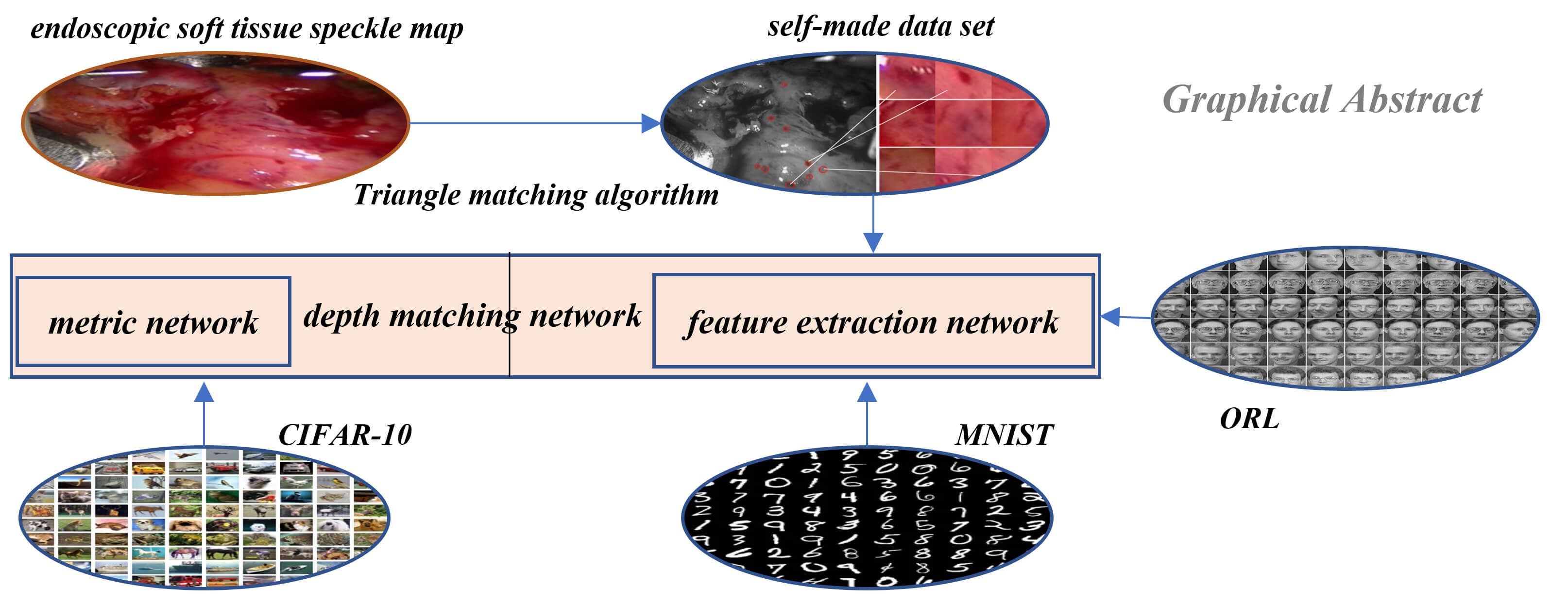
Research in the field of medical image is an important part of the medical robot to operate human organs. A medical robot is the intersection of multi-disciplinary research fields, in which medical image is an important direction and has achieved fruitful results. In this paper, a method of soft tissue surface feature tracking based on a depth matching network is proposed. This method is described based on the triangular matching algorithm. First, we construct a self-made sample set for training the depth matching network from the first N frames of speckle matching data obtained by the triangle matching algorithm. The depth matching network is pre-trained on the ORL face data set and then trained on the self-made training set. After the training, the speckle matching is carried out in the subsequent frames to obtain the speckle matching matrix between the subsequent frames and the first frame. From this matrix, the inter-frame feature matching results can be obtained. In this way, the inter-frame speckle tracking is completed. On this basis, the results of this method are compared with the matching results based on the convolutional neural network. The experimental results show that the proposed method has higher matching accuracy. In particular, the accuracy of the MNIST handwritten data set has reached more than 90%.Graphic Abstract
Keywords
In recent years, surgical robots have begun to be frequently used in minimally invasive surgery to reduce the pain of patients, reduce the work intensity of the surgeon, improve the accuracy of surgical operations, and reduce the difficulty of surgical operations [1–4]. This operation is mainly used for disease monitoring and treatment of various parts of the human body through an endoscope, which enters the human body through a small channel (a natural channel or a channel confirmed by a doctor). Compared with traditional surgery, the position perception of intraoperative equipment and soft tissue surface requires high accuracy, and because the intraoperative field of view is relatively narrow, it causes a lot of difficulties [5]. Therefore, many computer-assisted techniques have been proposed to assist the operation process [6,7], and many advanced robot-assisted surgical techniques have extremely high requirements for the tracking of the soft tissue surface characteristics of the surgical organs, such as abnormal brain detection method for magnetic resonance image and detecting tuberculosis from chest CT images [8,9]. Tracking research on the surface of soft tissue is conducive to the use of surgical robots’ high-precision and high-flexibility characteristics. It can perform precise surgical operations in different organs and tissues of the human body [10–12]. It is conducive to the recovery and reconstruction of surgical organs and tissues, greatly reduces the danger caused by the shaking of the body during the operation of the surgeon, greatly enhances the doctor’s confidence and reduces the surgeon’s fatigue, and enhances the safety and effectiveness of the operation. In addition, the tracking of soft tissue surface features of endoscopic image sequences has very important applications in postoperative surgical effect analysis, surgical training and teaching, and virtual reality soft tissue 3D modeling [11,13].
The tracking problem in the medical field is a hot issue [14], and most of the technical routes adopted are based on the feature as the object to launch the tracking. However, problems such as low matching accuracy and slow speed of feature points in endoscopic images remain.
Recent research has revealed that image-based methods can enhance accuracy and safety in laser microsurgery. Schoob et al. proposed a non-rigid tracking using surgical stereo imaging [15]. A recently developed motion estimation framework based on piecewise affine deformation modeling is extended by a mesh refinement step and considers texture information. This compensates for tracking inaccuracies potentially caused by inconsistent feature matches or drift. To facilitate the online application of the method, the computational load is reduced by concurrent processing and affine-invariant fusion of the tracking and refinement results. The residual latency-dependent tracking error is further minimized by Kalman filter-based upsampling, considering a motion model in disparity space.
The surface feature of the soft tissue image is used as the tracking object to realize the tracking of the surface of the soft tissue [16]. The key step of the soft tissue surface feature tracking process is feature matching. The feature matching method is also applied to feature matching in different views of the same frame. At a certain moment, the coordinates of a three-dimensional space point are mapped to two different perspective images in the left and right views, but they are actually the same space point. Similarly, feature matching is performed on the points of the left and right views to obtain the parallax under different viewing angles. In addition, the internal and external parameters of the camera that shoots the left and right views and the focal length are added to obtain the three-dimensional coordinates of the space points.
Robotic automation in surgery requires the precise tracking of surgical tools and mapping of deformable tissue. Previous works on surgical perception frameworks require significant effort in developing features for surgical tools and tissue tracking. In this work, Lu et al. [17] overcame the challenge by exploiting deep learning methods for surgical perception. They integrated deep neural networks, capable of efficient feature extraction, into the tissue tracking and surgical tool tracking processes. By leveraging transfer learning, the deep-learning-based approach requires minimal training data and reduced feature engineering efforts to fully perceive a surgical scene.
Verdie et al. [18] proposed a learning-based time invariant feature detector (TILDE), which can reliably detect key points in the case of severe changes in external conditions such as illumination. An effective method is proposed to generate the training set of training regression. This method learns three regressors, and the segmented regressor shows the best effect. The author evaluates the regressor on the new outdoor benchmark data set, which shows that the performance of the regressor proposed by the author on the benchmark data set is obviously better than the most excellent algorithm at that time. Savinov et al. proposed Quartnetworks [19]. They first proposed to learn the feature detector from scratch, train a neural network to rank the key points, and then find the key points from the top/bottom bits of the ranking. The workflow of the whole method is to extract random block pairs from two images. Each image block obtains a response through the neural network, then calculates the loss through the sorting consistency function of quadruple and optimizes it by gradient descent method. The algorithm based on data learning can not only learn the feature detector like Quarknetworks, but also learn the feature descriptor. With the improvement of machine learning [20–24], Simoserra et al. proposed Deepdesc [25] for key point descriptor learning. This method uses a convolutional neural network to learn the discriminant representation of image blocks (patches), trains a Siamese network with paired inputs, and processes a large number of paired image blocks by combining the random extraction of training sets and the mining strategy for patch pairs that are difficult to classify. The L2 distance is used in training and testing, and the learned 128-d descriptor is used. Its Euclidean distance reflects the similarity of patch pairs. The feature learning method maps the pixel values of image blocks to description vectors through nonlinear coding. The goal is to learn description vectors. The selection of measurement rules of these description vectors is generally related to the real label vector. The processing process of references [26,27] included multiple parameterization modules such as gradient calculation, spatial pooling, feature normalization and dimension reduction. Trzcinski et al. [28] used a “weak learning” accelerator, including a series of capabilities of gradient direction and spatial position parameterization. In order to find the optimal parameters, different types of optimization algorithms, Powell minimization, boosting and convex optimization are used respectively.
Feature based 3D reconstruction is the last step of soft tissue surface tracking, mainly to build a visual object model with more three-dimensional spatial characteristics. The key point of 3D reconstruction technology is feature matching. In the stereo matching of binocular vision, the corresponding points in space are obtained from the two-dimensional feature matching results and camera parameters, combined with the triangular knowledge of epipolar geometry, multiple feature matching, and then the three-dimensional point cloud set of multiple points is obtained. Finally, the three-dimensional shape of the soft tissue surface is restored through triangulation. The essence of soft tissue surface reconstruction is to accurately estimate the object’s three-dimensional shape. It is a process of converting a two-dimensional image into a three-dimensional image based on feature point matching data. In [29], the authors proposed an intraoperative surface reconstruction method based on stereo endoscope images. At the same time, the author also proposed a new hybrid CPU-GPU algorithm, which unifies the advantages of CPU and GPU versions. An innovative synchronous positioning and mapping algorithm is proposed in [30], which used a series of images of the stereo mirror to reconstruct the surface deformably. The author introduced a distortion field based on embedded deformation nodes, which can restore the three-dimensional shape from continuous paired stereo images.
In this paper, we used the feature matching algorithm based on deep learning, mainly based on the soft tissue tracking of the deep matching network. First, we used the triangle matching algorithm to obtain a self-made data set, then used the ORL face data set to pre-train the deep matching network, and then used the self-made training set to train the deep matching network. After carrying out the two-class feature tracking of the deep matching network, we carried out the multi-class spot tracking based on the convolutional neural network. In the multi-class convolutional neural network part, the same neural network architecture is used, and different pre-training sets, the MNIST handwritten data set and CIFAR-10 data set are used to experiment with the effect of the pre-training set on retraining and get the results. Finally, experiments are carried out on the algorithm of this paper and the influence of the network structure and training data set on the experimental results is analyzed and compared. The innovations are that we used three unrelated data sets to pre-train and retrain the matching network, constructed the training data set to prepare the training samples for the neural training network, improved the depth matching network based on the Siamese network and finally achieved good matching results.
The initialization parameters of the neural network are obtained by training on the ORL face data set [31]. The ORL face data set contains a total of 400 images of 40 different people. Each person has 10 different images. The light, facial expressions and details of the images are different, and the size is 112 * 92 grayscale images. The data set is shown in Fig. 1.
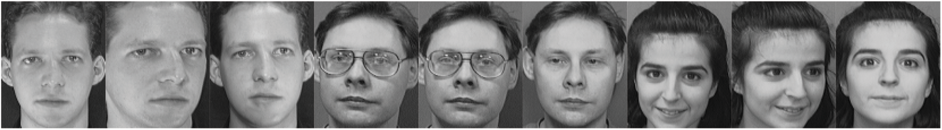
Figure 1: ORL face dataset
The two data sets used in the pre-training in this article are the MNIST data set and the CIFAR-10 data set [32,33]. The data set is shown in Figs. 2 and 3.
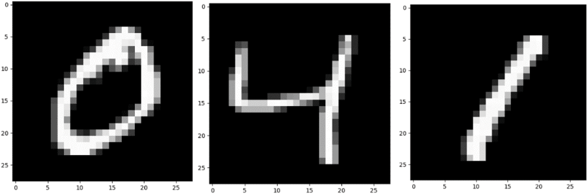
Figure 2: MNIST dataset
Firstly, the MNIST data set of handwritten scanned digits is introduced. NIST, on behalf of the National Institute of standards and technology, is the organization that originally collected these data “M” stands for modified. In order to use machine learning algorithm easier, we first preprocessed the data. The MNIST dataset includes scanning of handwritten digits and related labels (describing which number of 0∼9 is contained in each image). It includes 60000 training images with 28 * 28 pixels and 10000 test images with 28 * 28 pixels. As shown in Fig. 2, these handwritten digits are standardized in size and located in the center of the image, and the pixel value of the image is normalized to 0∼1.
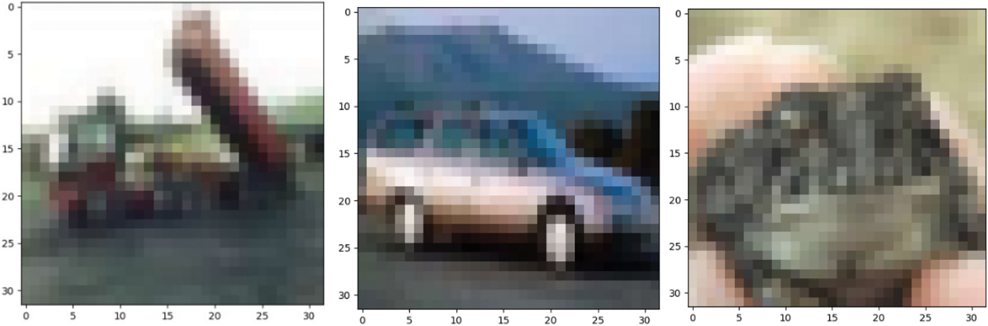
Figure 3: CIFAR-10 dataset
The CIFAR-10 dataset contains 10 categories, aircraft, cars, birds, cats, deer, dogs, frogs, horses, ships, and trucks. A total of 60000 RGB color images, including 50000 training images and 10000 test images.
Medical dataset we used in this paper is a set of actual three-dimensional images of the soft tissue of the heart provided by Hamlyn Center at Imperial College London. They are available on the website: https://imperialcollegelondon.app.box.com/s/kits2r3uha3fn7zkoyuiikjm1gjnyle3.
3.1 Triangular Matching Algorithm
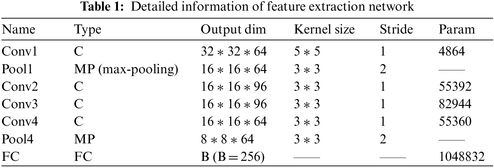
The constructed matching data set is shown in Fig. 4. The first frame is our known frame, as shown in the figure, the 25th and 30th frames are the data sets matched by our triangle matching algorithm. Because the spot detection algorithm is affected by light, etc., the triangle matching can not match the first frame one by one, and there is spot loss in the subsequent frame
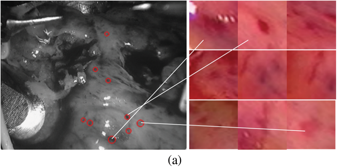
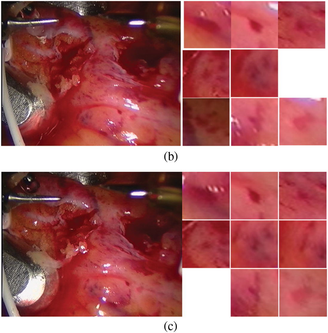
Figure 4: Screenshot and its spots (a) first frame (b) frame 25 (c) frame 30
3.2 Speckle Tracking Based on Depth Matching Network
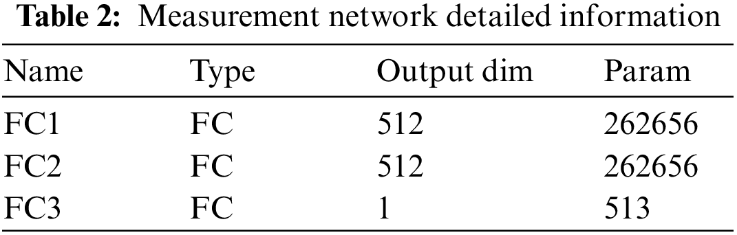
The depth matching network is mainly composed of two parts, feature extraction network and metric network. The feature extraction is composed of two convolutional neural networks [22,34] with shared weights. This thinking comes from the Siamese network and twin neural network, which is very suitable for the binary classification task of image matching. Each image block (patch) inputs a feature extraction network to generate a fixed dimension sift like feature. This feature is a depth feature, but different from sift, the similarity and difference between the two feature description vectors in sift are calculated by the Euclidean distance, while in depth matching network, the metric network is used.
The metric network consists of three fully connected layers. The last layer uses sigmoid function (i.e., Eq. (1)) to output scores to obtain the similarity probability of image blocks.
The feature extraction network includes five convolution layers and two lower sampling layers, and includes an FC layer used to reduce the dimension of the features extracted by the feature extraction network. The function of the FC layer is to reduce the feature dimension extracted by the feature extraction network and control the overfitting of the network, because the number of parameters involved in full connection is large. If the feature dimension is too high, it will easily lead to a large number of parameters and over fitting. The output 256 dimension of FC layer represents the advanced features of the input image block, and each image block represents the spots detected in the frame. Therefore, FC layer represents the spot depth features “integrated” by the feature extraction network.
Because our input image is small, the size of the convolution kernel we use is relatively small, which is also to comprehensively and carefully obtain the feature information in the image block (patch). The convolution kernel after filling and then convolution greatly increases the nonlinear characteristics without losing the resolution while keeping the scale of the feature map unchanged; A convolution kernel corresponds to a feature map after convolution. Different convolution kernels (with different weights and bias) will get different feature maps after convolution to extract different features.
We use the RELU (rectified linear units) function [35] as the activation function of the convolution layer. Similarly, the sign function of the full connection layer is also RELU. The introduction of the activation function is to increase the nonlinearity of the convolution layer. Without the activation function, each convolution layer is equivalent to matrix multiplication, and the output of each layer only goes through a linear transformation. No matter how many layers the neural network has, the linear transformation is of little significance as a whole. Obviously, we want to learn the nonlinear characteristics of image blocks. By adding an activation function, nonlinear changes are introduced into neurons, so the neural network can be used to simulate any nonlinear function arbitrarily.
The details of the depth matching network, such as parameters, convolution kernel size, convolution step size and so on, are listed in Tables 1 and 2.
After the detailed information description of the network layer is completed, we make necessary explanations for the training method. We select positive and negative samples with batch size from the training sample set to build a group of training samples. The number of positive and negative samples in each batch size is equal.
Depth matching network is based on minimizing the cross entropy loss function to train network parameters. The cross-entropy function [36] is:
where
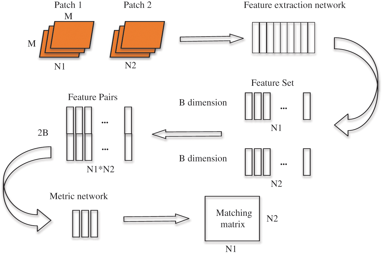
Figure 5: Schematic diagram of depth matching network training process
We calculate the matching matrix between
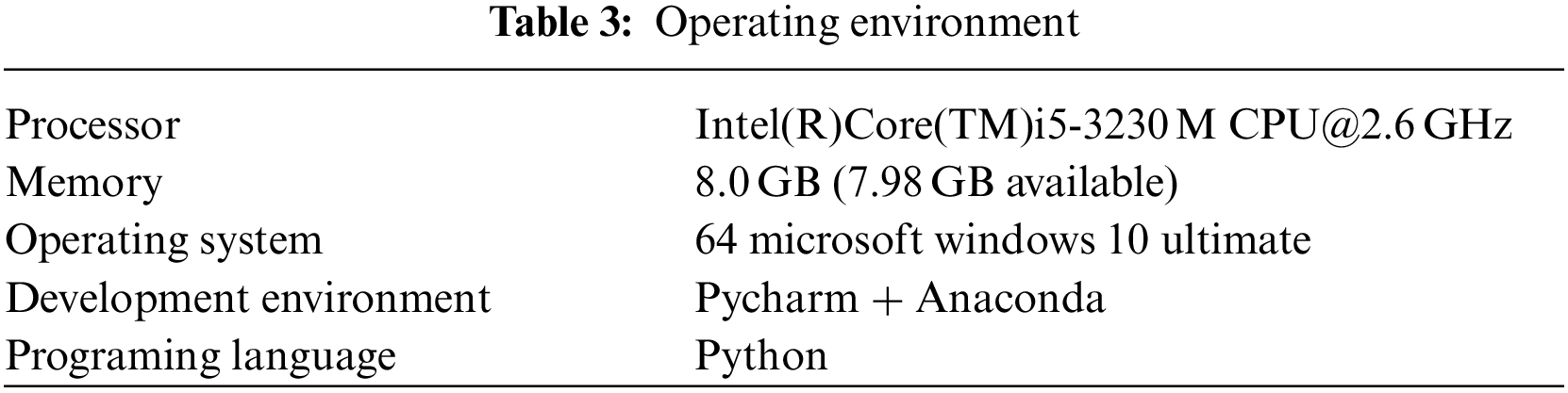
Our experiment is based on TensorFlow 2.1, python 3.7, NVIDIA Geforce GTX 1060ti and other platforms. The program running environment is shown in Table 3.
When constructing the sample set, we need to first expand the edges of the bottom of the input image. Our input picture is 288 * 320, and the spot coordinates near the bottom edge of the detected spots are close to the y value (288) in the picture coordinate system, where the origin of the picture coordinate system is in the upper left corner. The y-value index of the spot coordinate has the hidden danger of crossing the boundary. Therefore, before capturing the picture, fill in the bottom of the picture. In this article, we choose the boundary pixel extension [37], which is conducive to the feature extraction network to fully extract the pixel information around the spots. The edge filling result is shown in Fig. 6.
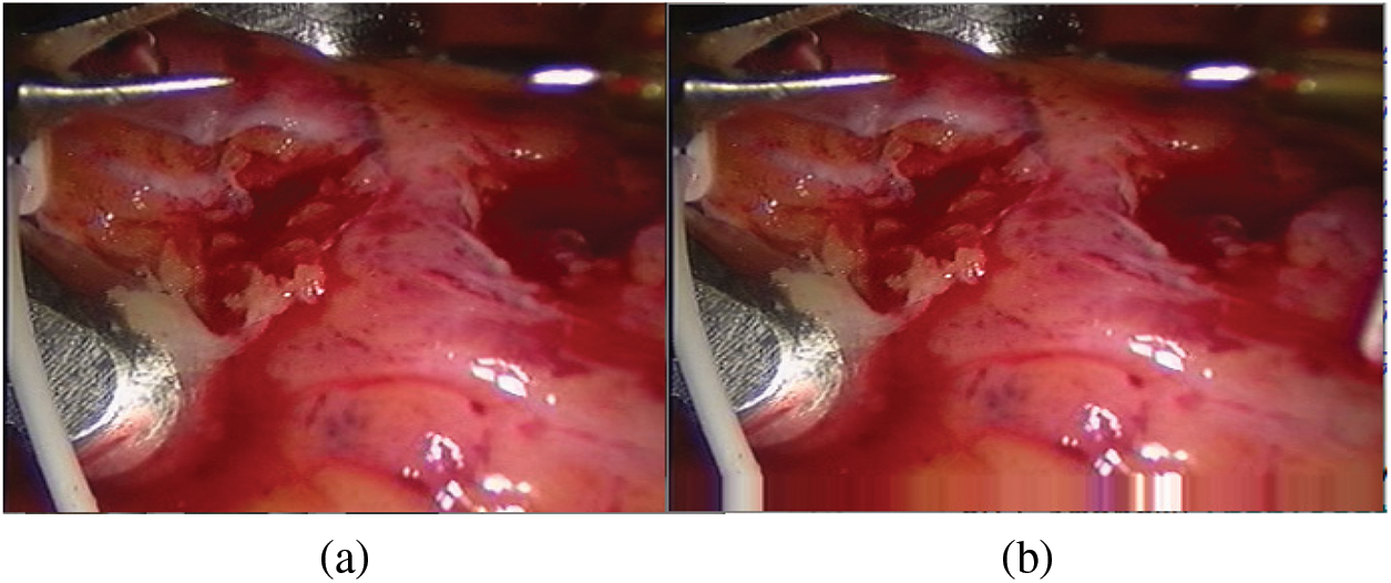
Figure 6: Bottom edge filling (a) Original drawing (b) Boundary pixel expansion
According to the feature point matching results of the first 100 frames, the image block with the size of M * M = 32 * 32 is intercepted with the position coordinates of the matched feature points as the center, and the positive samples and negative samples are constructed by combining them. The spots in the positive samples are the corresponding vertices of the two triangles matched with each other, marked as 1. The spots in the negative sample are the corresponding vertices of two mismatched triangles, marked as 0. Finally, all the positive and negative samples are used to construct the training sample set. For our proposed depth matching network, we use the network pre-training to obtain the initialization parameters in the network. The depth matching network is pretrained on ORL face data set. The pre-training results are shown in Fig. 7 and the re-training results are shown in Fig. 8. It can be seen from Figs. 7 and 8 that although the pre-training stage has performed well, under the retraining of the self-made training set, the curve is smoother and converges faster from the accuracy curve and loss curve. Therefore, the weight parameters obtained by pre-training are effective, which speeds up the training progress and convergence speed.
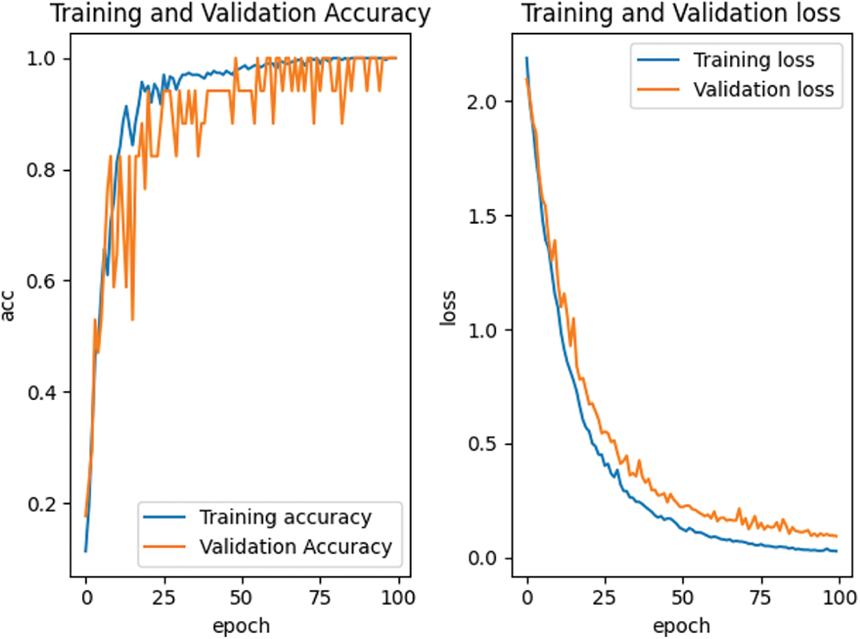
Figure 7: Accuracy and loss curve in pre-training stage
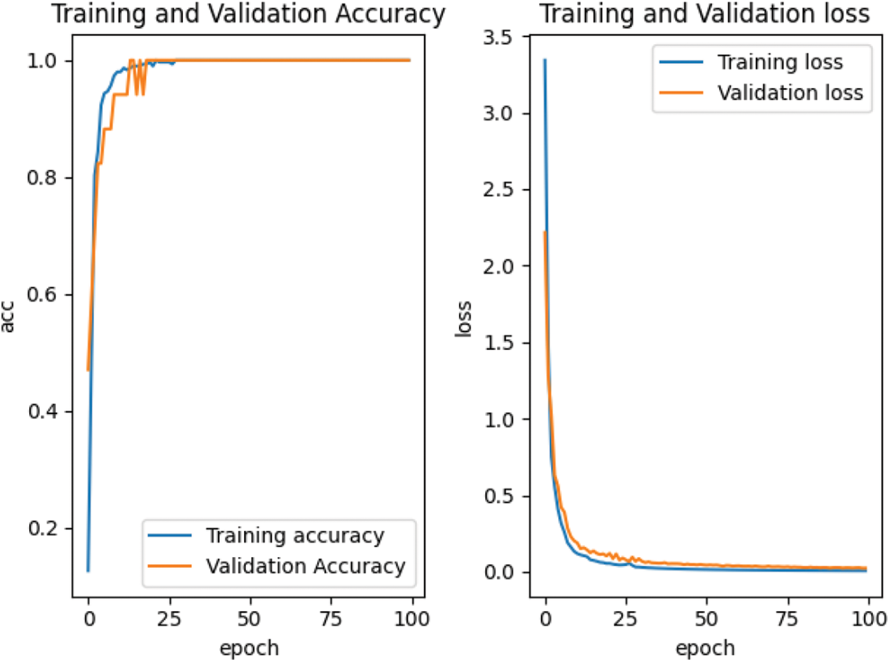
Figure 8: Accuracy and loss curve in retraining stage
For the traditional neural network, 32 * 32 * 3 endoscopic soft tissue speckle map is used as the input, and the previous n = 100 frame matching result is used as the training set. Due to the loss of spots, a total of 750 speckle maps are used as the training set, and 180 speckle images of the subsequent 20 frames are used as the test set to train and test the convolutional neural network.
The two data sets used for pre-training are the MNIST data set and the CIFAR-10 dataset. We will perform pre-training on the two data sets respectively, and then use our self-made training set for retraining. On the same network structure, different data sets are used for pre-training, and the influence of the pre-training data set on the convolutional neural network training can be compared; After the retraining stage, we can see the impact of pre-training on retraining.
In the network setting, the learning rate is 0.0001, the optimizer adopts Adam optimizer and small batch training method, batchsize = 32, and the maximum training epoch = 100. The training results are shown in Fig. 9.
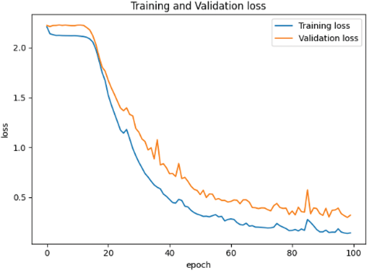
Figure 9: Loss reduction curve based on MNIST data set
When training the convolutional neural network based on CIFAR-10 data set, the input is changed from single channel gray image to 3-channel RGB image. The learning rate, optimizer and other parameter settings remain unchanged, and the training results are shown in Fig. 10.
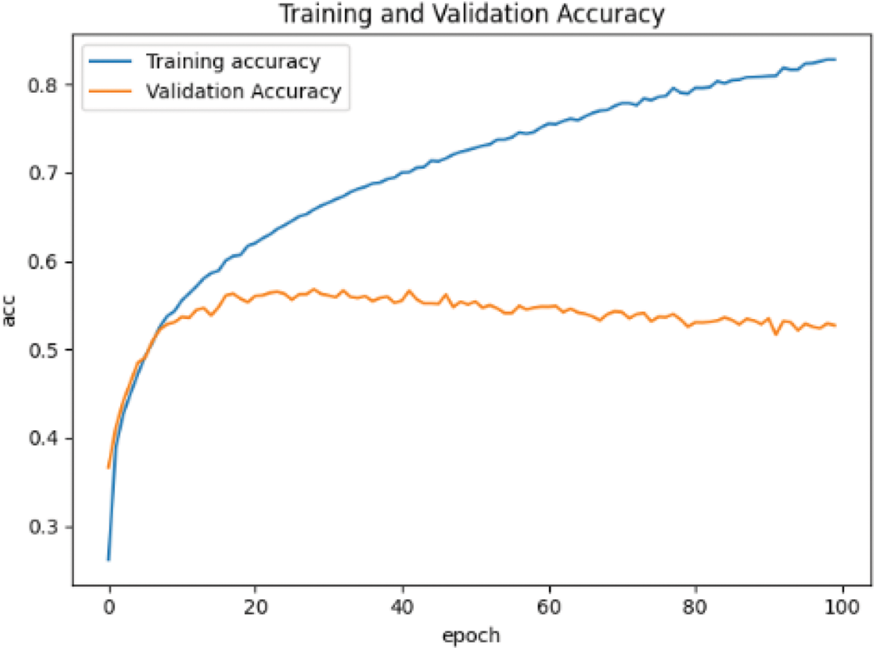
Figure 10: Accuracy curve based on CIFAR-10 data set
Save the weight of the pre-training and use the self-made training set for retraining. The results of retraining are shown in Fig. 11.
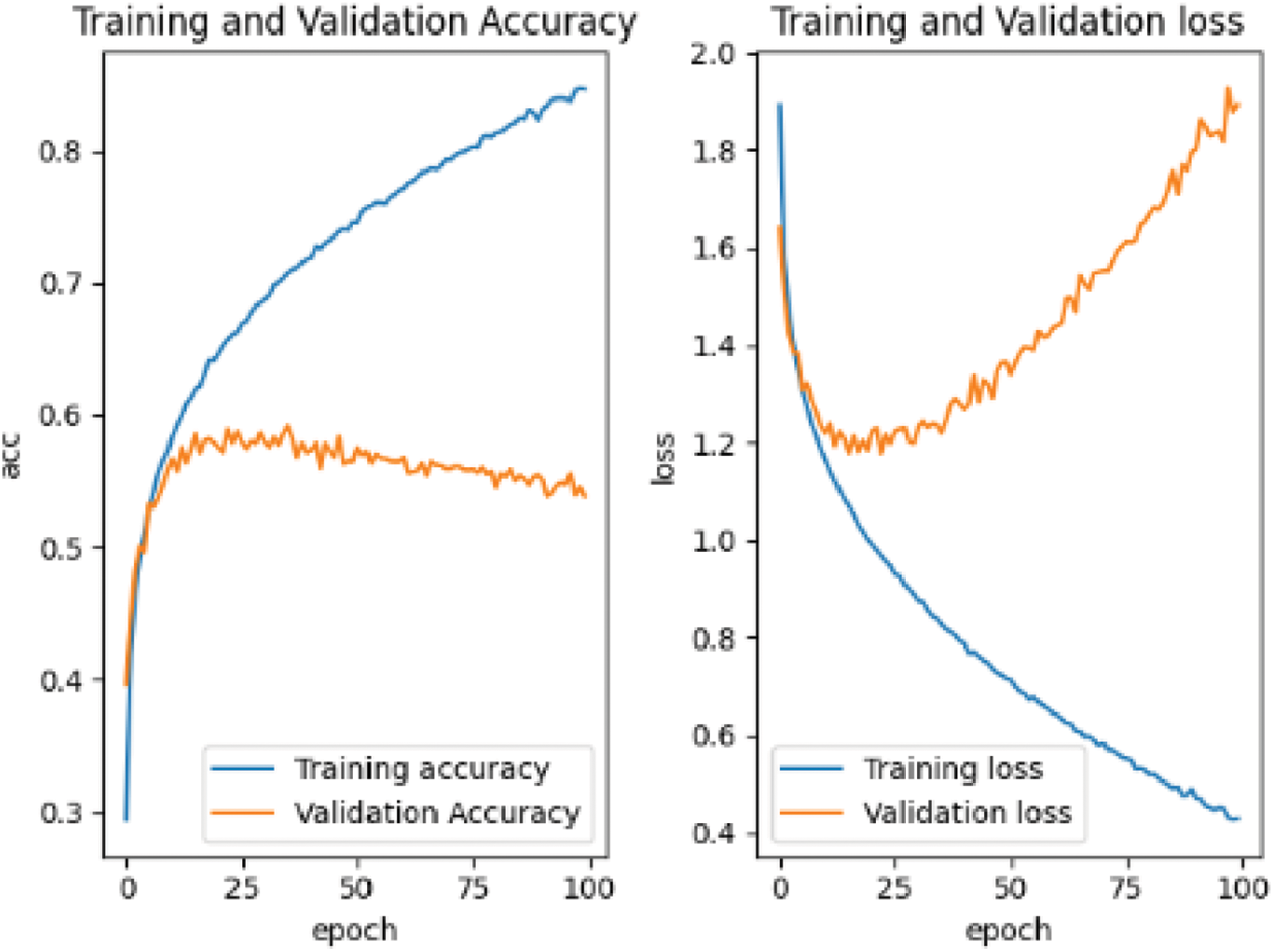
Figure 11: Retraining loss and accuracy curve based on CIFAR-10 data set
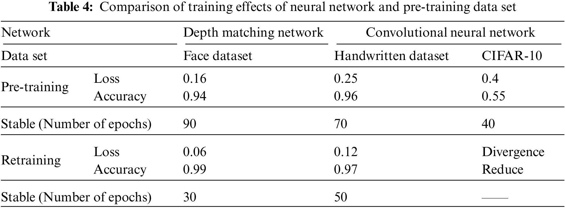
As mentioned in the previous paper, we use three different data sets to study inter frame speckle matching on two neural networks. The differences between neural networks and the comparison of data sets are shown in Table 4.
In the subsequent frames, in order to ensure the universality of the test, any frame is selected. In the experiment, any frame selected by the program is
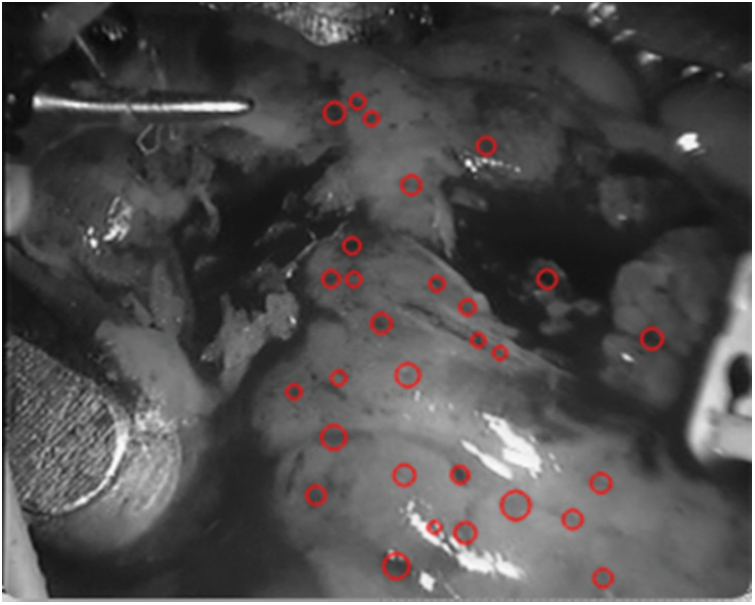
Figure 12: Detection spot map in
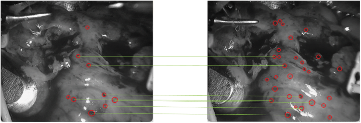
Figure 13: Speckle matching diagram obtained by matching score matrix
Spot 1 is most stably detected in the first frame, so we still track spot 1 in subsequent frames, as shown in Fig. 14, which shows the tracking of spots with serial number 1 detected in the first frame. The horizontal axis is the number of frames, the vertical axis is the pixel coordinate of the spot,the vertical axis of the left figure is the X coordinate of the pixel coordinate, and the vertical axis of the right figure is the Y coordinate of the pixel coordinate. The origin of pixel coordinates is located in the upper left corner of the image, and the X and Y of pixel coordinates are just opposite to the row and column values of accessing the two-dimensional image matrix.
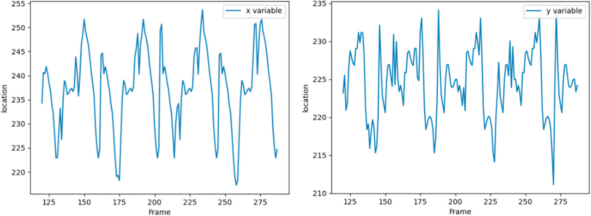
Figure 14: Pixel coordinate tracking results of subsequent frames of speckle 1
From Figs. 9 and 10, the accuracy of the two data sets in the pre-training stage is different. The accuracy of the MNIST handwritten data set has reached more than 90%, which can be considered that the purpose of pre-training has been achieved. However, the accuracy rate on the CIFAR-10 data set is only 50%, and even the accuracy of the test set tends to decline.
As can be seen from Fig. 12, retraining has obvious divergence and overfitting. The reason is that the pre-training of the pre-training data set is not in place. We can also see from the pre-training curve that its accuracy curve and the trend of decline appear. Only the pre-training sample set is large, and it may continue to be pre-trained for hundreds of rounds, which will be the same as that of retraining. In the complex feature information, the pre-trained sample data set has a considerable impact on the subsequent retraining.
It can be seen from Figs. 10–12 that the grid multi-classification effect based on CIFAR-10 data set is obviously inferior to that based on the MNIST handwritten data set. It shows that the pre-training of the data set still has a significant impact on the subsequent retraining.
It can be seen from Table 4 that in the pre-training stage, the training results of the depth matching network on the face data set are excellent. If we continue to use the self-made training set, the convergence is faster, the accuracy curve is steeper, and its initial starting point is also relatively high, It shows that the weight parameter obtained by pre-training on the gray image face data set is an effective weight parameter for soft tissue image speckle training set, and shortens the retraining time; Convolutional neural network also performs well on MNIST handwritten gray-scale images, but it performs poorly on the RGB CIFAR-10 data set for two reasons: the first reason is that the characteristics of the MNIST handwritten digits are as simple as those of soft tissue image surface spots, and the gray-scale information is regional, while the image information of cars, animals and other images in CIFAR-10 data set is more complex, And the characteristics of surface spots in soft tissue images; The second reason is that the structure of convolutional neural network itself is relatively simple, which can only deal with images with simple feature information. For complex feature information such as images in CIFAR-10 dataset, it is easy to overfit, resulting in non-convergence or even divergence.
As shown in Fig. 12, it can be seen that the spots detected in
In the experiment, spot 1 is tracked from frame 121. From the pixel coordinates, the heartbeat range is still about 30 pixels, which means that the soft tissue feature tracking algorithm based on depth matching network is successful.
This paper constructs the training data set to prepare the training samples for the neural training network. After that, we improve the depth matching network based on the Siamese network to adapt to the feature extraction and measurement of soft tissue surface images. Firstly, we pre-train on the ORL face data set to get better results and then retrain on our own data set to get a smoother and steeper loss curve and accuracy curve so as to achieve the purpose of retraining. Furthermore, we compared the spot-matching algorithms of classified convolutional neural networks. In terms of convolutional neural networks, Lenet was used as the basic structure and slightly modified, pre-trained on the MNIST handwritten data set and the CIFAR-10 data set respectively, and then retrained with a self-made training set. The pre-training based on the MNIST data set performed well in the retraining stage. However, the pre-training accuracy based on the CIFAR-10 data set reaches 50%, and the loss in the retraining stage shows a divergent form, and the accuracy decreases significantly. It can be seen that the data set has a significant impact on the results of pre-training and retraining. Therefore, in the follow-up research, we can further select more data sets to train the deep matching network for better performance.
Acknowledgement: Thank all the authors for their contributions to the paper.
Funding Statement: This work was jointly supported by the Sichuan Science and Technology Program (Grant: 2021YFQ0003; Acquired by Wenfeng Zheng).
Conflicts of Interest: The authors declare that they have no conflicts of interest to report regarding the present study.
References
1. Zhang, W., Yao, G., Yang, B., Zheng, W., Liu, C. (2022). Motion prediction of beating heart using spatio-temporal LSTM. IEEE Signal Processing Letters, 29, 787–791. DOI 10.1109/LSP.2022.3154317. [Google Scholar] [CrossRef]
2. Guo, F., Yang, B., Zheng, W., Liu, S. (2021). Power frequency estimation using sine filtering of optimal initial phase. Measurement, 186, 110165. DOI 10.1016/j.measurement.2021.110165. [Google Scholar] [CrossRef]
3. Tang, Y., Liu, S., Deng, Y., Zhang, Y., Yin, L. et al. (2020). Construction of force haptic reappearance system based on geomagic touch haptic device. Computer Methods and Programs in Biomedicine, 190, 105344. DOI 10.1016/j.cmpb.2020.105344. [Google Scholar] [CrossRef]
4. Deng, Y., Tang, Y., Yang, B., Zheng, W., Liu, S. et al. (2021). A review of bilateral teleoperation control strategies with soft environment. 2021 6th IEEE International Conference on Advanced Robotics and Mechatronics (ICARM), pp. 459–464. Chongqing, China. [Google Scholar]
5. Zlatintsi, A., Dometios, A. C., Kardaris, N., Rodomagoulakis, I., Koutras, P. et al. (2020). I-support: A robotic platform of an assistive bathing robot for the elderly population. Robotics and Autonomous Systems, 126, 103451. DOI 10.1016/j.robot.2020.103451. [Google Scholar] [CrossRef]
6. Zheng, W., Yang, B., Xiao, Y., Tian, J., Liu, S. et al. (2022 Apr 9). Low-dose CT image post-processing based on learn-type sparse transform. Sensors, 22(8), 2883. DOI 10.3390/s22082883. [Google Scholar] [CrossRef]
7. Xu, S., Yang, B., Xu, C., Tian, J., Liu, Y. et al. (2022). Sparse angle CBCT reconstruction based on guided image filtering. Frontiers in Oncology, 12, 832037. DOI 10.3389/fonc.2022.832037. [Google Scholar] [CrossRef]
8. Lu, S., Wang, S. H., Zhang, Y. D. (2020). Detection of abnormal brain in MRI via improved AlexNet and ELM optimized by chaotic bat algorithm. Neural Computing and Applications, 33, 10799–10811. [Google Scholar]
9. Lu, S. Y., Wang, S. H., Zhang, X., Zhang, Y. D. (2021). TBNet: A context-aware graph network for tuberculosis diagnosis. Computer Methods and Programs in Biomedicine, 214, 106587. [Google Scholar]
10. Li, Y., Zheng, W., Liu, X., Mou, Y., Yin, L. et al. (2021). Research and improvement of feature detection algorithm based on FAST. Rendiconti Lincei. Scienze Fisiche e Naturali, 32(4), 775–789. DOI 10.1007/s12210-021-01020-1. [Google Scholar] [CrossRef]
11. Zhang, Z., Liu, Y., Tian, J., Liu, S., Yang, B. et al. (2021). Study on reconstruction and feature tracking of silicone heart 3D surface. Sensors, 21(22), 7570. DOI 10.3390/s21227570. [Google Scholar] [CrossRef]
12. Liu, S., Wang, L., Liu, H., Su, H., Li, X. et al. (2018). Deriving bathymetry from optical images with a localized neural network algorithm. IEEE Transactions on Geoscience and Remote Sensing, 56(9), 5334–5342. DOI 10.1109/TGRS.36. [Google Scholar] [CrossRef]
13. Yang, B., Liu, C., Zheng, W., Liu, S., Huang, K. (2018). Reconstructing a 3D heart surface with stereo-endoscope by learning eigen-shapes. Biomedical Optics Express, 9(12), 6222–6236. DOI 10.1364/BOE.9.006222. [Google Scholar] [CrossRef]
14. Schwab, K., Smith, R., Brown, V., Whyte, M., Jourdan, I. (2017). Evolution of stereoscopic imaging in surgery and recent advances. World Journal of Gastrointestinal Endoscopy, 9(8), 368–377. DOI 10.4253/wjge.v9.i8.368. [Google Scholar] [CrossRef]
15. Schoob, A., Kundrat, D., Kahrs, L. A., Ortmaier, T. (2017). Stereo vision-based tracking of soft tissue motion with application to online ablation control in laser microsurgery med. Medical Image Analysis, 40, 80–95. DOI 10.1016/j.media.2017.06.004. [Google Scholar] [CrossRef]
16. Yang, B., Liu, C., Huang, K., Zheng, W. (2017). A triangular radial cubic spline deformation model for efficient 3D beating heart tracking. Signal, Image and Video Processing, 11(7), 1329–1336. DOI 10.1007/s11760-017-1090-y. [Google Scholar] [CrossRef]
17. Lu, J., Jayakumari, A., Richter, F., Li, Y., Yip, M. C. (2021). SuPer deep: A surgical perception framework for robotic tissue manipulation using deep learning for feature extraction. 2021 IEEE International Conference on Robotics and Automation (ICRA), pp. 4783–4789. Xi'an, China. DOI 10.1109/ICRA48506.2021.9561249. [Google Scholar] [CrossRef]
18. Verdie, Y., Yi, K. M., Fua, P., Lepetit, V. (2015). TILDE: A temporally invariant learned DEtector. 2015 IEEE Conference on Computer Vision and Pattern Recognition (CVPR), pp. 5279–5288. DOI 10.1109/CVPR.2015.7299165. [Google Scholar] [CrossRef]
19. Savinov, N., Seki, A., Ladicky, L., Sattler, T., Pollefeys, M. (2017). Quad-networks: Unsupervised learning to rank for interest point detection. 2017 IEEE Conference on Computer Vision and Pattern Recognition (CVPR), Honolulu, HI, USA. [Google Scholar]
20. Dankwa, S., Zheng, W. (2019). Special issue on using machine learning algorithms in the prediction of kyphosis disease: A comparative study. Applied Sciences, 9(16), 3322. DOI 10.3390/app9163322. [Google Scholar] [CrossRef]
21. Xu, J., Liu, Z., Yin, L., Liu, Y., Tian, J. et al. (2021). Grey correlation analysis of haze impact factor PM2.5. Atmosphere, 12, 1513. DOI 10.3390/atmos12111513. [Google Scholar] [CrossRef]
22. Wang, Y., Tian, J., Liu, Y., Yang, B., Liu, S. et al. (2021). Adaptive neural network control of time delay teleoperation system based on model approximation. Sensors, 21(22), 7443. DOI 10.3390/s21227443. [Google Scholar] [CrossRef]
23. Chen, H., Chen, J., Ding, J. (2021). Data evaluation and enhancement for quality improvement of machine learning. IEEE Transactions on Reliability, 70(2), 831–847. DOI 10.1109/TR.2021.3070863. [Google Scholar] [CrossRef]
24. Sheth, S., Lee, P., Bajaj, A., Cuchel, M., Hajj, J. (2021). Implementation of a machine-learning algorithm in the electronic health record for targeted screening for familial hypercholesterolemia: A quality improvement study. Circulation: Cardiovascular Quality and Outcomes, 14, e007641. DOI 10.1161/CIRCOUTCOMES.120.007641. [Google Scholar] [CrossRef]
25. Simoserra, E., Trulls, E., Ferraz, L., Kokkinos, I., Fua, P. et al. (2016). Discriminative learning of deep convolutional feature point descriptors. 2015 IEEE International Conference on Computer Vision (ICCV), pp. 118–126. Santiago, Chile. [Google Scholar]
26. Brown, M., Hua, G., Winder, S. (2010). Discriminative learning of local image descriptors. IEEE Transactions on Pattern Analysis & Machine Intelligence, 33(1), 43–57. DOI 10.1109/TPAMI.2010.54. [Google Scholar] [CrossRef]
27. Simonyan, K., Vedaldi, A., Zisserman, A. (2014). Learning local feature descriptors using convex optimisation. IEEE Transactions on Pattern Analysis and Machine Intelligence, 36(8), 1573–1585. DOI 10.1109/TPAMI.2014.2301163. [Google Scholar] [CrossRef]
28. Trzcinski, T., Christoudias, M., Lepetit, V. (2012). Learning image descriptors with the boosting-trick. IEEE Transactions on Pattern Analysis and Machine Intelligence, 37(3), 1. [Google Scholar]
29. Rohl, S., Bodenstedt, S., Suwelack, S., Dillmann, R., Speidel, S. et al. (2012). Dense GPU-enhanced surface reconstruction from stereo endoscopic images for intraoperative registration. Medical Physics, 39(3), 1632–1645. DOI 10.1118/1.3681017. [Google Scholar] [CrossRef]
30. Song, J., Wang, J., Zhao, L., Huang, S., Dissanayake, G. (2018). Dynamic reconstruction of deformable soft-tissue with stereo scope in minimal invasive surgery. IEEE Robotics & Automation Letters, 4(1), 33–40. DOI 10.1109/LRA.2018.2876888. [Google Scholar] [CrossRef]
31. Dubey, S. R., Mukherjee, S. (2018). A multi-face challenging dataset for robust face recognition. 2018 15th International Conference on Control, Automation, Robotics and Vision (ICARCV), pp. 168–173. Singapore. DOI 10.1109/ICARCV.2018.8581283. [Google Scholar] [CrossRef]
32. Lu, J., Batra, D., Parikh, D., Lee, S. (2019). ViLBERT: Pretraining task-agnostic visiolinguistic representations for vision-and-language tasks. arXiv:1908.02265. [Google Scholar]
33. Cao, J., Gan, Z., Cheng, Y., Yu, L., Chen, Y. et al. (2020). Behind the scene: Revealing the secrets of pre-trained vision-and-language models. Cham: Springer. [Google Scholar]
34. Huang, R., Li, J., Wang, S., Li, G., Li, W., (2020). A robust weight-shared capsule network for intelligent machinery fault diagnosis. IEEE Transactions on Industrial Informatics, 16(10), 6466–6475. DOI 10.1109/TII.2020.2964117. [Google Scholar] [CrossRef]
35. Tian, Y. (2020). Artificial intelligence image recognition method based on convolutional neural network algorithm. IEEE Access, 8, 125731–125744. DOI 10.1109/ACCESS.2020.3006097. [Google Scholar] [CrossRef]
36. Ding, Y., Tian, X., Yin, L., Chen, X., Liu, S. et al. (2019). Multi-scale relation network for few-shot learning based on meta-learning. International Conference on Computer Vision Systems, pp. 343–352. Cham, Springer. [Google Scholar]
37. Dong, Z., Li, J., Fang, T., Shao, X. (2021). Lightweight boundary refinement module based on point supervision for semantic segmentation. Image and Vision Computing, 110, 104169. DOI 10.1016/j.imavis.2021.104169. [Google Scholar] [CrossRef]
Cite This Article
 Copyright © 2023 The Author(s). Published by Tech Science Press.
This work is licensed under a Creative Commons Attribution 4.0 International License , which permits unrestricted use, distribution, and reproduction in any medium, provided the original work is properly cited.
 Downloads
 Citation Tools