Nonlinear Flow Properties of Newtonian Fluids through Rough Crossed Fractures

1  Introduction

In deep rock masses, Darcy’s law and cubic law are typically applied to estimate the hydraulic properties of engineering sites, which are only applicable for fluids in a linear flow regime with a sufficiently small flow velocity [1,2]. When the inertial effects are not negligible with a relatively high flow velocity, the fluid flow is within the nonlinear flow regime and Darcy’s law and cubic law are not suitable. Instead, the nonlinear flow governing equations of fluids, such as Navier-Stokes equations, should be solved [3,4]. The nonlinear fluid flow through single fractures has been studied in the past decades to some extent [5–8]. However, the fracture networks are composed of single fractures and fracture intersections. Therefore, the nonlinear fluid flow through crossed fractures that can be regarded as a simple fracture network should also be investigated.

Kosakowski et al. [9] numerically solved Navier-Stokes equations to examine the variabilities of flow patterns in artificial fracture intersection geometries. They reported that the nonlinear inertial effects play an important role when the Reynolds number is as low as 1–100, which commonly exists in natural karst systems and the vicinity of wells during pump tests. Johnson et al. [10] carried out flow and solute transport experiments through epoxy replicas of intersecting natural fractures. The results show that surface roughness–induced aperture variability in the intersecting fractures may allow pure fingers of one solution to cross straightly through the intersection and block the flow from the adjacent inlet. Johnson et al. [11] developed a numerical method for solute mixing in fracture intersections, which agrees well with the experimental results both in average mixing amount and dye streamline distributions. They concluded that the roughness of fracture surfaces enhances the mixing to a great extent by reducing solute dilution and increasing solute dispersion. Liu et al. [12] investigated the effect of intersection on nonlinear flow properties of crossed fractures, both experimentally and numerically. They reported that when the Reynolds number of the inlet is larger than 1, the nonlinear flow regime appears and the ratio of flow rates between the two outlets changes nonlinearly. Zou et al. [13] presented numerical modeling of fluid flow and solute transport in rock fracture-matrix systems, in which the intersection is formed by two rough-walled fractures. They found that the channeling of fluid flow can significantly influence the mixing processes at the intersections. Li et al. [14] addressed the significance of surface roughness on fluid flow and solute transport through crossed rock fractures by numerically solving the Navier-Stokes equations. The results show that the previously widely used smooth parallel-plate computational domain deviates greatly in predicting the solute transport properties within crossed fractures. This is because in the natural cases, the intersections are formed by unmated fracture surfaces. However, in the above studies, there are still two unsolved issues. On the one hand, the nonlinear flow properties of fluids through intersections are not characterized, although the Navier-Stokes equations are solved. On the other hand, although the nonlinear fluid flow is considered and investigated, the intersection geometry is simple or a small number of influencing factors are taken into consideration. Thus, it is of special importance to systematically study the nonlinear streamline distributions and nonlinear fluid flow properties through crossed fractures by considering the effects of length, aperture, and surface roughness of fractures.

In the present study, the nonlinear flow of Newtonian fluids through crossed fractures is simulated using 36 computational domains. The model length changes from 20 to 100 mm and the fracture aperture varies from 1 to 5 mm. The fracture surface roughness coefficient (JRC) is within the range of 3.20–20.91. The hydraulic gradient varies from 10−6 to 100 spanning 7 orders of magnitude. The nonlinear relationships between flow rate and hydraulic gradient, as well as the variations in the ratio of flow rate to hydraulic gradient, are analyzed. Finally, the empirical expression of critical hydraulic gradient that can quantify the onset of nonlinear fluid flow is proposed as a function of the length and aperture of fractures.

2  Theoretical Backgrounds

The Navier-Stokes equations and continuity equation as shown in Eqs. (1) and (2) can be solved to model the flow of incompressible Newtonian fluids through rock fractures [15,16]

ρ[∂u/∂t+(u⋅∇)u]=−∇p+∇⋅T+ρf(1)

∇⋅u=0(2)

where u is the flow velocity tensor, ρ is the fluid density, p is the hydraulic pressure tensor, T is the shear stress tensor, t is the time, and f is the body force tensor.

Eqs. (1) and (2) are vector equations containing four unknowns and solving them without any restrictions is not an easy task. By assuming (i) the fluid flow velocity is relatively small, (ii) the two walls of a fracture are smooth and parallel, (iii) the fluid flow is in a steady-state, (iv) there are no-slip boundaries, (v) the dimension in the aperture direction is much smaller than that in the other two perpendicular directions, (vi) the hydraulic head loss along the aperture direction is negligible, Eq. (1) can be reduced to the following cubic law [17]:

Q=−we312μΔPΔL(3)

where Q is the flow rate, w is the width of fractures, e is the hydraulic aperture, μ is the dynamic viscosity, L is the fracture length.

Eq. (3) can also be written in the form of

−ΔPΔL=aQ(4)

where a is the linear coefficient.

When the flow velocity is relatively large and the inertial force cannot be negligible compared with the viscous force, the nonlinear term bQ2 should be added to the right term of Eq. (4), which is the famous Forchheimer’s law as follows [18–20]:

−ΔPΔL=aQ+bQ2(5)

where b is the nonlinear coefficient. Note that Eq. (5) is an empirical function, which cannot be directly derived from Eq. (1) or Eq. (3).

Since the hydraulic gradient (J) defined as the ratio of water head difference to the length of a fracture (Δh/ΔL) is linearly proportional to ΔP/ΔL, Eqs. (4) and (5) can be re-written as

−J=a′Q(6)

−J=a′Q+b′Q2(7)

where a’ = a/(ρg) and b’ = b/(ρg), respectively. Eq. (7) is Forchheimer’s law–based equation. Note that the typical Forchheimer’s law is not directly used because the hydraulic pressure drop in the left term of Eq. (5) is not a dimensionless parameter. However, the J in the left term of Eq. (7) is a dimensionless parameter, which can be used to quantify the flow regimes of fluids that can consider the scale effect.

For a fixed computational domain, with the increment of J, the flow velocity increases and fluid flow transits from a linear regime to a nonlinear regime. The critical hydraulic gradient (Jc) is defined to quantify the onset of the nonlinear flow of fluids, below which the fluid flow is in the linear regime and above which the fluid flow is in the nonlinear flow regime.

3  Computational Domains and Calculation Procedures

Fig. 1 shows schematic illustrations of the computational domains with different mechanical apertures (E), JRC, and L. The first two lines present computational domains with L = 100 mm. The third and fourth lines show computational domains with L = 50 mm. The last two lines exhibit computational domains with L = 20 mm. The E equals 5, 2, and 1 mm, and the JRC equals 3.20, 11.21, 14.08, and 20.91, respectively. The JRC is calculated by the following Eqs. (8) and (9) [21,22]:

JRC=32.2+32.47logZ2(8)

Z2=[1M∑(zi−1−zixi−1−x)2]1/2(9)

where Z2 is typical fracture surface roughness parameter, M is the number of sampling point along the length direction, xi and zi are the coordinates of the fracture surface profile.

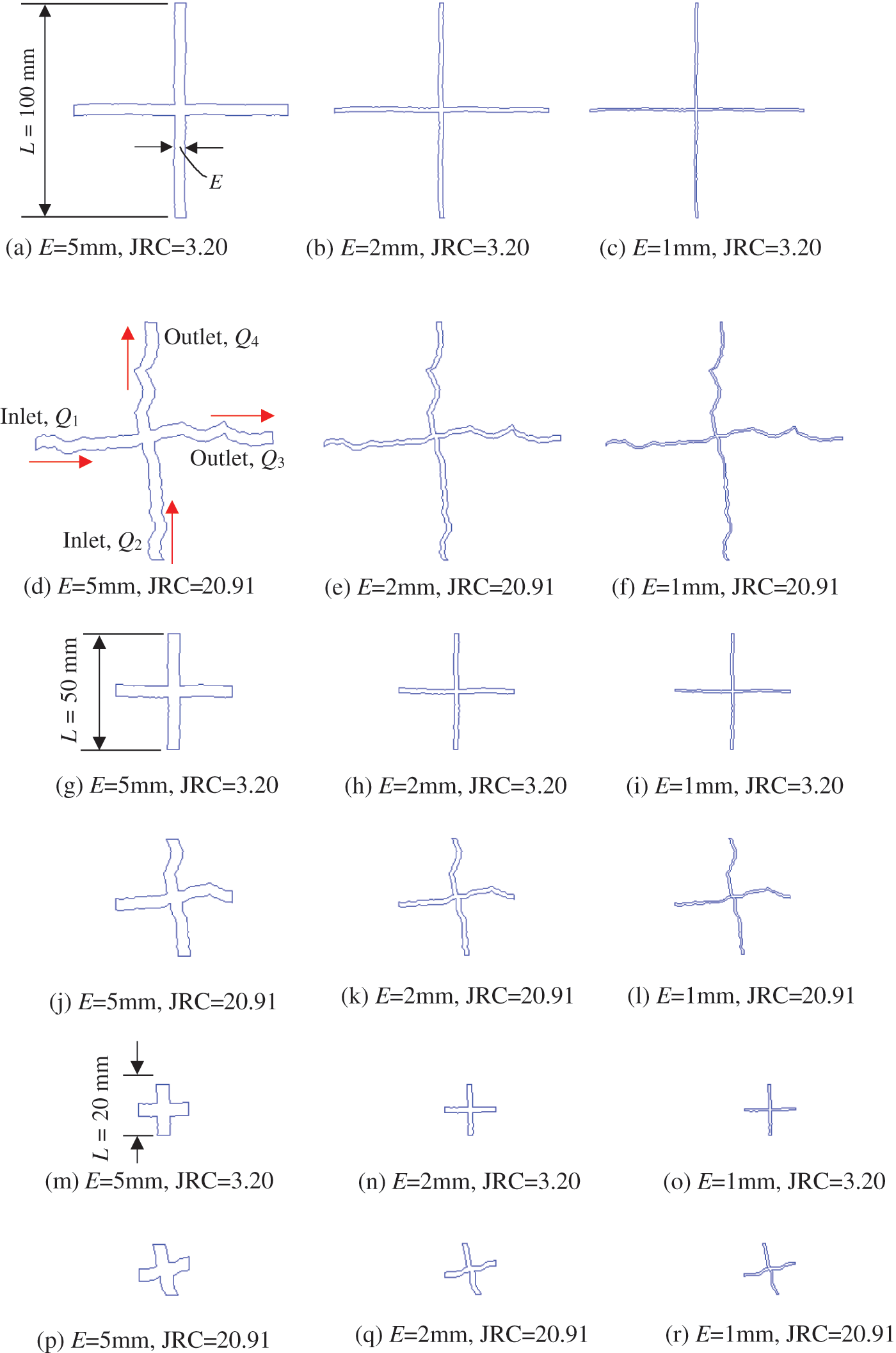
Figure 1: Crossed fractures with different E, JRC, and L. The first two lines present computational domains with L = 100 mm, and the third and fourth lines show computational domains with L = 50 mm, while the last two lines exhibit computational domains with L = 20 mm

In the present study, the JRC of fractures with L = 100 mm is calculated. The JRC of fractures with smaller sizes, such as L = 50 and 20 mm, are not calculated and the values are assumed to be equal to those for L = 100 mm. The rough surfaces of fractures are from or cut from the Barton curves [23], which show curves with different JRCs. The two walls of a fracture are assumed to be well-mated with a distance of E. The two fractures are perpendicular to each other. The computational domains with L = 50 and 20 mm are extracted from the central parts of the computational domains with L = 100 mm. Therefore, a total of 36 computational domains were prepared. Note that only two JRC structures of the upper bound and lower bound with JRC = 3.20 and 20.91 are presented. The other two JRC structures with JRC = 11.21 and 14.08 that are within the two bounds are not presented for simplification. However, the variations in the Q/J and normalized Q/J vs. J for all cases are presented and discussed in the following analysis.

The fluid is assumed to flow into the computational domain through two adjacent inlets and out of the computational domain through the other two adjacent outlets, as shown in Fig. 1d. The same boundary conditions have been widely accepted in previous works such as Johnson et al. [11], Kosakowski et al. [9] and Zou et al. [13]. The other boundaries of the fractures are assumed to be non-slip and impermeable. The fluid flow process is simulated with the help of ANSYSFLUENT module, which is a commercial software. The Navier-Stokes equations are solved using the finite element volume (FVM) method. Initially, the same hydraulic pressure is applied on the two inlets and the hydraulic pressure of both outlets equals zero. When the fluid flow is in a steady state, the total flow rate Q = Q1 + Q2 = Q3 + Q4. The pressure-based solver is used and the SIMPLE scheme is chosen for the modeling. It has been reported that when the number of layers along the aperture direction is larger than 20, the numerical simulation can have a relatively high accuracy [24]. Therefore, in the present study, the number of layers along the aperture direction is chosen to be 25. As a result, the maximum meshing size is 0.2, 0.08, and 0.04 mm for the computational domains with E = 5, 2, and 1 mm, respectively, when the quadrilateral meshes are used. Taking the case of E = 5 mm, JRC = 20.91, and L = 100 mm as an example, there are a total of 28099 meshes and 26066 nodes, and it takes about 16 min for the calculation. The numerical simulation method for modeling nonlinear fluid flow through rock fractures using the ANSYS FLUENT module has been verified to be valid in our previous works ([12]; [24–26]), which is not repeatedly presented here. To fully cover both the linear and nonlinear flow regimes, the J is applied spanning 7 orders of magnitude, which varies from 10−6 to 100 for the 36 computational domains. Therefore, a total of 252 computational runs are performed and fluid flow processes are simulated. The water at room temperature is used as the fluids, which has a density of 998.2 kg/m3 and a viscosity of 0.001 Pa·s.

4  Results and Analysis

4.1 Nonlinear Q–J Relationships

Fig. 2 presents the nonlinear Q–J relationships for L = 100 mm (the first line), 50 mm (the second line) and 20 mm (the third line) with JRC = 3.20 (the first column) and 20.91 (the last column), indicating that the fluid flow is in the strongly nonlinear regime. The Q has a quadratic relationship with J having a zero-intercept, following Eq. (7). With the decrease in L from 100 to 20 mm, the Q decreases for a fixed J (i.e., J = 100). This is because the intersection plays a more significant role in the energy losses than the fracture segment. When the geometry of the intersection is fixed and the length of fracture segments increases, the degree of energy loss decreases, and the permeability/conductivity increases. As a result, the Q is larger for a longer L when J is fixed. All curves clearly show that with increasing E from 1 to 5 mm, the Q increases. As JRC increases, the Q decreases when J is fixed. This is reasonable because the larger JRC, the rougher fracture surface and the more energy losses.

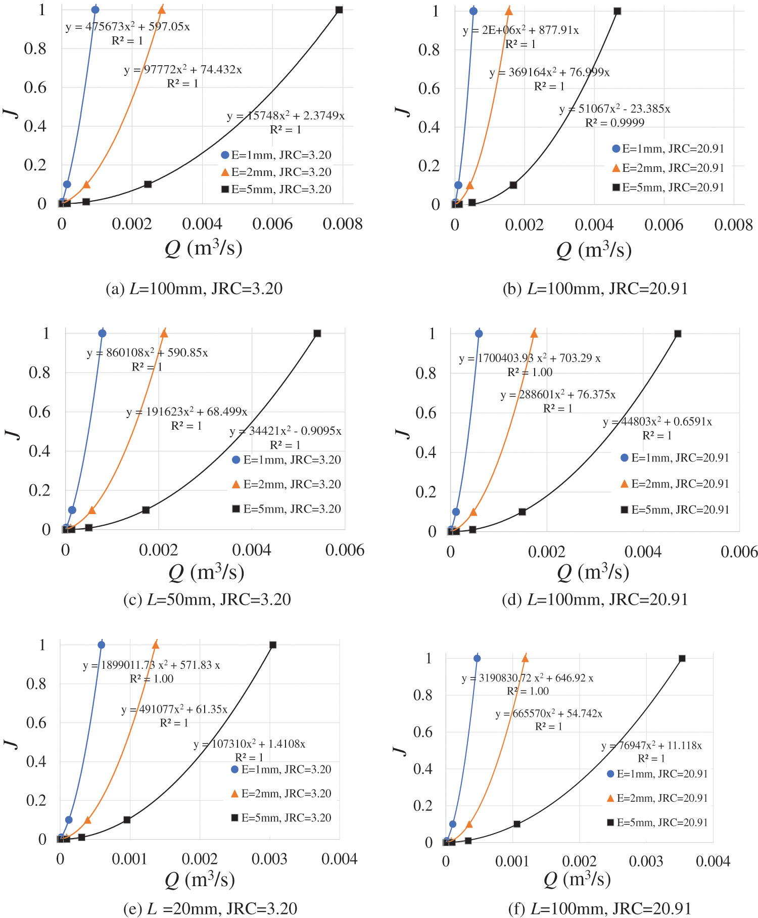
Figure 2: Q–J curves for L = 100 mm (the first line), 50 mm (the second line) and 20 mm (the third line) with JRC = 3.20 (the first column) and 20.91 (the last column)

However, the decrease degree in Q induced by the increment of JRC decreases with the increase in L. For example, when L = 50 mm, the Q varies slightly when JRC = 3.20–20.91. The Q evenly increases with the increment of JRC when L = 20 mm. This is because the small computational domains are extracted from the large computational domains. Thus, the JRC of fractures in small-scale computational domains may vary with respect to that of large-scale computational domains. For example, when L = 20 mm, the actual surface roughness of fractures with JRC = 20.91 does not differ significantly from that of JRC = 3.20. So, the effect of JRC decreases for a relatively small L.

4.2 Nonlinear Streamline Distributions

Fig. 3 exhibits the streamline distributions for crossed fractures with different E, JRC, L, and J. (a)–(f) show the smaller computational domains extracted from the original large computational domains, with streamline distributions for different J. (g)–(j) compare the streamline distributions with different E and J. When J = 10−6, the streamlines are parallel to the walls of fractures and smoothly move from the inlets to the outlets. There are no eddies formed because the inertial forces are negligible and fluid flow is in the linear flow regime. When J = 100, the fluid flow enters the nonlinear flow regime and obvious eddies exist in the outlet branches, which is induced by the significant effect of inertial force. However, the eddies are not formed in the inlets. With the increment of L from 20 to 100 mm, the streamline distributions do not change robustly for J = 10−6. However, the streamline distributions including the number of eddies and eddy distributions change significantly for J = 100. Such changes will influence the nonlinear hydraulic properties of fluid flow.

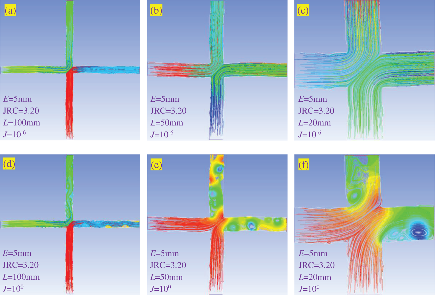
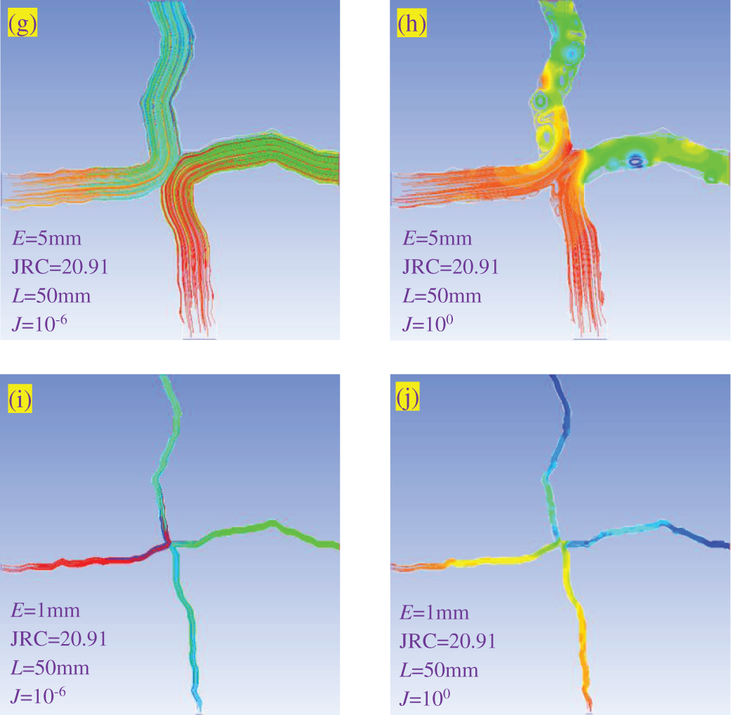
Figure 3: Streamline distributions for crossed fractures with different E, JRC, L, and J. (a)–(f) show the smaller computational domains extracted from the original large computational domains, with streamline distributions for different J. (g)–(j) compare the streamline distributions with different E and J

Figs. 3b, 3e, 3g, and 3h depict the effect of JRC on the streamline distributions by fixing E = 5 mm and L = 50 mm. When J = 10−6, the streamlines are rougher for a larger JRC, whereas the streamlines are still parallel to the walls of fractures. When J = 100, the eddies are mostly formed in the outlets with a smaller number of eddies formed in the inlets. With the increment of JRC, the number of eddies increases for both inlets and outlets, due to that the change in fracture walls will promote the formation of eddies. Therefore, it is understandable that the larger JRC, the more energy losses and the smaller permeability/conductivity. Figs. 3g–3j show the streamline distributions with E varying from 1 to 5 mm when JRC = 20.91 and L = 50 mm. When J = 10−6, the streamline distributions are the same as those shown in Figs. 3a–3c. When J = 100, the magnitude of eddies decreases with the decrease in E because the small E narrows the void spaces for fluid flow. The ratio of the area occupied by eddies to the other area decreases with decreasing E. Therefore, the E can also affect the streamline distributions and nonlinear hydraulic properties of crossed fractures, depending on surface roughness and length of fractures.

4.3 Variations in Q/J

As shown in Eq. (6), Q/J is a constant when fluid flow is in the linear flow regime. When fluid flow enters the nonlinear flow regime, Eq. (7) is applicable. Q/J, which decreases with increasing J (or Q), is no longer a constant. Therefore, the variations in Q/J vs. J can be utilized to quantify the nonlinear flow characterizations of fluids. Figs. 4a–4c show the variations in Q/J vs. J varying from 10−6 to 100 with L = 100, 50, and 20 mm, respectively. The results show that when J < 10−5, the values of Q/J are constants, despite of the magnitude of J. In such a case, Eq. (6) can be used to simulate fluid flow. When 10−5 < J < 10−3, the Q/J decreases slightly and fluid flow enters the weak nonlinear flow regime. With continuously increasing J (i.e., J > 10−3), the Q/J decreases significantly and fluid flow enters the strong nonlinear flow regime. As E increases from 1 to 5 mm, the Q/J increases robustly because the Q/J is proportional to the permeability of fractures. When L = 100 mm, the Q/J decreases as the JRC increases from 3.20 to 20.91, due to the increase in the tortuous flow length. However, the decreasing degree induced by JRC decreases as L decreases (i.e., from 100 to 20 mm). Fig. 4d shows the effect of JRC on Q/J for different L. With the increment of JRC from 3.20 to 14.08, the variations in Q/J are almost the same in both the trends and magnitudes for L = 20–100 mm. When JRC = 3.20–14.08, the Q/J decreases from 0.00165 to 0.00147 m3/s, from 0.00164 to 0.00143 m3/s, and from 0.00165 to 0.00145 m3/s by rates of 11.38%, 12.94% and 12.17% for L = 100, 50 and 20 mm, respectively. For JRC = 14.08–20.91, the variations in Q/J for L = 50 and 20 mm are similar, which however are different from those for L = 100 mm. The Q/J decreases from 0.00143 to 0.00133 m3/s and from 0.00145 to 0.00134 m3/s by rates of 7.19% and 7.65% for L = 50 and 20 mm, respectively, whereas the Q/J decreases from 0.00147 to 0.00106 by a rate of 27.87% for L = 100 mm. This indicates that the JRC plays a more important role in a larger computational domain. This can also be reflected in Fig. 1 that the surfaces of fractures are rougher for a larger computational domain. However, the effect of JRC vanishes for a relatively small computational domain (i.e., L = 20 mm).

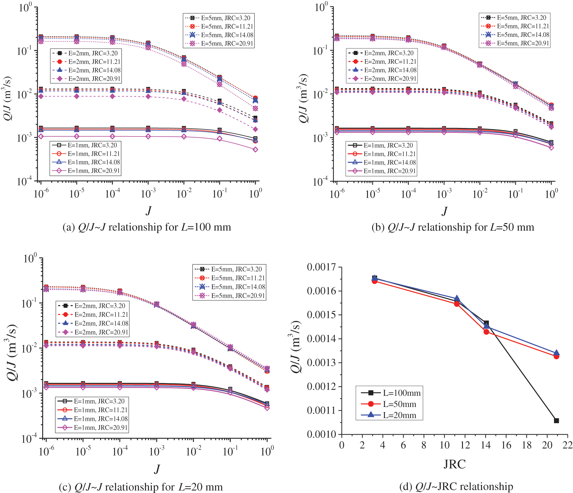
Figure 4: (a)–(c) Variations in Q/J vs. J varying from 10−6 to 100 with L = 100, 50, and 20 mm, respectively; (d) Effect of JRC on Q/J with different L

4.4 Determination of Jc

As mentioned in the above section, the variations in Q/J can be used to quantify the nonlinear flow of fluids through crossed fractures. The normalized Q/J is defined as the ratio of Q/J to the initial Q/J, where the initial Q/J corresponds to the value of Q/J for fluid flow in the linear flow regime. In the present work, the initial Q/J is calculated for J = 10−6. The variations in normalized Q/J vs. J are plotted in Figs. 5a–5c. With the increment of J, the normalized Q/J decreases, depending on the values of L and E, whereas the JRC plays a negligible role. The normalized Q/J that equals to 0.9 is adopted as the critical value that fluid flow transits from a linear regime to a nonlinear regime. The corresponding J is the critical hydraulic gradient (Jc) [27]. The results show that Jc increases with decreasing E and increasing L as presented in Fig. 5d. The Jc has power-law relationships with E, as follows:

Jc=mE−n(10)

where m and n are coefficients correlating to L. The validity of Eq. (10) can be verified by comparisons with the results reported by Liu et al. [28], which shows a good agreement. The data are obtained from Liu et al. [28] when the number of intersections is 1.

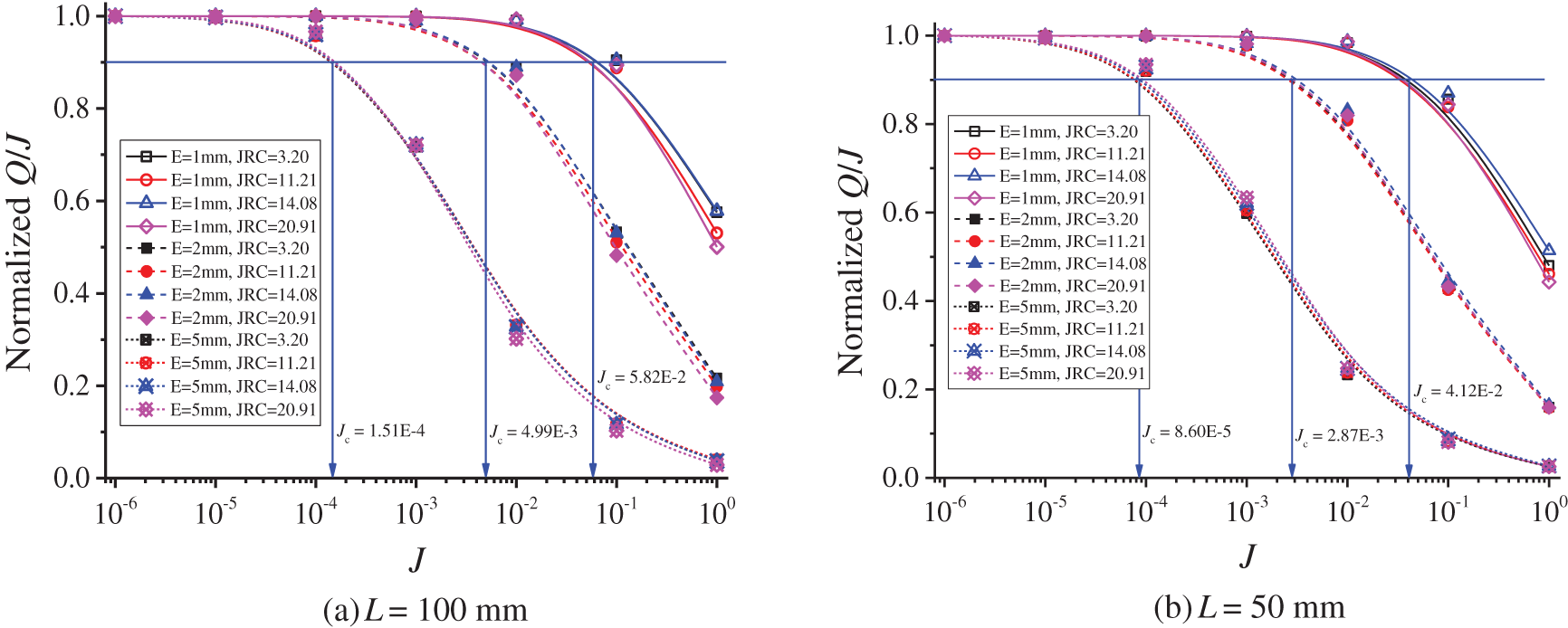
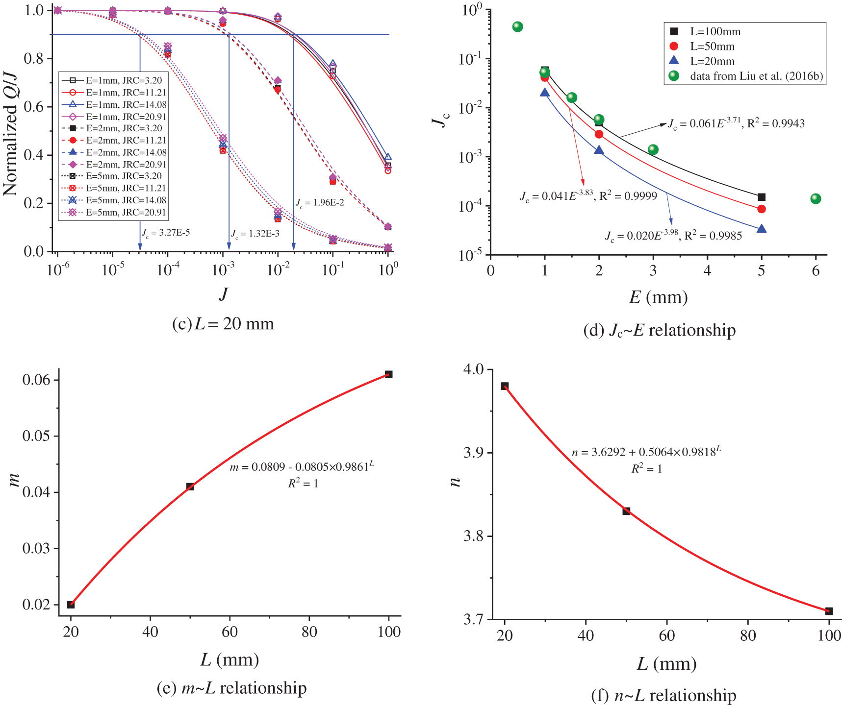
Figure 5: (a)–(c) Variations in normalized Q/J vs. J varying from 10−6 to 100 with L = 100, 50, and 20 mm, respectively; (d) Effect of E on Jc with different L; (e) Variations in m as a function of L; (f) Variations in n as a function of L

The variations in m and n vs. L are plotted in Figs. 5e and 5f, following exponential functions as:

m=0.0809−0.0805×0.9861L(11)

n=3.6292+0.5064×0.9818L(12)

Substituting Eqs. (11) and (12) into Eq. (10) yields the expression of Jc as a function of E and L, as follows:

Jc=(0.0809−0.0805×0.9861L)E−(3.6292+0.5064×0.9818L)(13)

Note that Eq. (13) is an empirical function and the unit of L is mm. Eq. (13) can be used to calculate Jc as long as E and L are determined. Here, Jc is utilized to quantify the onset of nonlinear fluid flow through fractures. As shown in Figs. 5a–5c, the Jc is more significantly influenced by E and L than JRC. In other words, although the JRC can influence the streamline distributions, the effect of JRC on Jc is negligible. Therefore, as a first-order estimation of Jc, the JRC is not taken into account.

5  Conclusions

The present study investigated the effects of length, aperture and surface roughness of fractures on the streamline distributions and nonlinear hydraulic properties of fluids through crossed fractures. The nonlinear relationships between flow rate and hydraulic gradient, the variations in the ratio of flow rate to hydraulic gradient vs. hydraulic gradient, and empirical expressions of critical hydraulic gradient as functions of length, aperture, and surface roughness of fractures, are analyzed and discussed.

The results show that the flow rate has quadratic relationships with hydraulic gradient with a zero intercept, indicating that the fluid flow is in the nonlinear flow regime. The larger hydraulic gradient, the stronger nonlinearity of fluid flow. The relationships between flow rate and hydraulic gradient move rightwards with increasing aperture and move downwards with the increasing length of computational domains. The streamlines are continuous from inlets to outlets for a relatively small hydraulic gradient, i.e., 10−6, while the streamlines are disturbed by eddies when the hydraulic gradient is relatively large, i.e., 100. The patterns of nonlinear streamlines, as well as the number and magnitude of eddies, depend on the associated parameters such as length, aperture, and surface roughness of fractures. As the hydraulic gradient increases, the fluid flow experiences a linear flow regime (hydraulic gradient = 10−6–10−5), a weak nonlinear flow regime (hydraulic gradient = 10−5–10−3), and a strong nonlinear flow regime (hydraulic gradient = 10−3–100). The joint roughness coefficient significantly influences the ratio of flow rate to hydraulic gradient, yet has a negligible effect on the critical hydraulic gradient. The critical hydraulic gradient is correlated with the fracture aperture, following power-law functions. The linear coefficient and the exponent coefficient are both correlated to the length of computational domains. The critical hydraulic gradient can be determined as function of fracture aperture and length of computational domains.

Although the effects of length, aperture, and surface roughness of fractures of crossed fractures are considered, the present study assumed that the two walls of fractures are well-mated. The anisotropy of the local aperture induced by shear or pressure solution should be taken into account to facilitate the expressions of the critical hydraulic gradient in future works. Besides, the size effect on the evolutions of JRC and corresponding hydraulic properties should be studied in the future.

Funding Statement: This study has been partially funded by National Key Research and Development Program of China, China (Grant No. 2020YFA0711800), Natural Science Foundation of China, China (Grant Nos. 51979272 and 51879150), Natural Science Foundation of Jiangsu Province, China (Grant No. BK20211584), Xuzhou Science and Technology Planning Project, China (Grant No. KC21004). These supports are gratefully acknowledged.

Conflicts of Interest: The authors declare that they have no conflicts of interest to report regarding the present study.

References

    1. Long, J. C. S., Remer, J. S., Wilson, C. R., Witherspoon, P. A. (1982). Porous media equivalents for networks of discontinuous fractures. Water Resources Research, 18(3), 645–658. DOI 10.1029/WR018i003p00645. [Google Scholar] [CrossRef]

    2. Min, K. B., Jing, L., Stephansson, O. (2004). Determining the equivalent permeability tensor for fractured rock masses using a stochastic REV approach: Method and application to the field data from sellafield, UK. Hydrogeology Journal, 12 (5), 497–510. DOI 10.1007/s10040-004-0331-7. [Google Scholar] [CrossRef]

    3. Chen, Y. F., Hu, S. H., Hu, R., Zhou, C. B. (2015). Estimating hydraulic conductivity of fractured rocks from high-pressure packer tests with an Izbash’s law-based empirical model. Water Resources Research, 51(4), 2096–2118. DOI 10.1002/2014WR016458. [Google Scholar] [CrossRef]

    4. Zhou, J. Q., Hu, S. H., Fang, S., Chen, Y. F., Zhou, C. B. (2015). Nonlinear flow behavior at low reynolds numbers through rough-walled fractures subjected to normal compressive loading. International Journal of Rock Mechanics and Mining Sciences, 80, 202–218. DOI 10.1016/j.ijrmms.2015.09.027. [Google Scholar] [CrossRef]

    5. Koyama, T., Neretnieks, I., Jing, L. (2008). A numerical study on differences in using Navier–Stokes and reynolds equations for modeling the fluid flow and particle transport in single rock fractures with shear. International Journal of Rock Mechanics and Mining Sciences, 45(7), 1082–1101. DOI 10.1016/j.ijrmms.2007.11.006. [Google Scholar] [CrossRef]

    6. Xiong, X., Li, B., Jiang, Y., Koyama, T., Zhang, C. (2011). Experimental and numerical study of the geometrical and hydraulic characteristics of a single rock fracture during shear. International Journal of Rock Mechanics and Mining Sciences, 48(8), 1292–1302. DOI 10.1016/j.ijrmms.2011.09.009. [Google Scholar] [CrossRef]

    7. Javadi, M., Sharifzadeh, M., Shahriar, K., Mitani, Y. (2014). Critical reynolds number for nonlinear flow through rough-walled fractures: The role of shear processes. Water Resources Research, 50(2), 1789–1804. DOI 10.1002/2013WR014610. [Google Scholar] [CrossRef]

    8. Liu, R., Huang, N., Jiang, Y., Jing, H., Yu, L. (2020). A numerical study of shear-induced evolutions of geometric and hydraulic properties of self-affine rough-walled rock fractures. International Journal of Rock Mechanics and Mining Sciences, 127, 104211. DOI 10.1007/s12303-015-0057-7. [Google Scholar] [CrossRef]

    9. Kosakowski, G., Berkowitz, B. (1999). Flow pattern variability in natural fracture intersections. Geophysical Research Letters, 26(12), 1765–1768. DOI 10.1029/1999GL900344. [Google Scholar] [CrossRef]

  10. Johnson, J., Brown, S. (2001). Experimental mixing variability in intersecting natural fractures. Geophysical Research Letters, 28(22), 4303–4306. DOI 10.1029/2001gl013446. [Google Scholar] [CrossRef]

  11. Johnson, J., Brown, S., Stockman, H. (2006). Fluid flow and mixing in rough-walled fracture intersections. Journal of Geophysical Research: Solid Earth, 111(B12), B12206. DOI 10.1029/2005JB004087. [Google Scholar] [CrossRef]

  12. Liu, R., Jiang, Y., Li, B. (2016a). Effects of intersection and dead-end of fractures on nonlinear flow and particle transport in rock fracture networks. Geosciences Journal, 20(3), 415–426. DOI 10.1007/s12303-015-0057-7. [Google Scholar] [CrossRef]

  13. Zou, L., Jing, L., Cvetkovic, V. (2017). Modeling of flow and mixing in 3D rough-walled rock fracture intersections. Advances in Water Resources, 107, 1–9. DOI 10.1016/j.advwatres.2017.06.003. [Google Scholar] [CrossRef]

  14. Li, B., Mo, Y., Zou, L., Liu, R., Cvetkovic, V. (2019). Influence of surface roughness on fluid flow and solute transport through 3D crossed rock fractures. Journal of Hydrology, 582, 124284. DOI 10.1016/j.jhydrol.2019.124284. [Google Scholar] [CrossRef]

  15. Bear, J. (1972). Dynamics of fluids in porous media. London: Elsevier. [Google Scholar]

  16. Zhou, J. Q., Li, C. D., Wang, L. C., Tang, H. M., Zhang, M. (2021). Effect of slippery boundary on solute transport in rough-walled rock fractures under different flow regimes. Journal of Hydrology, 598, 126456. DOI 10.1016/j.jhydrol.2021.126456. [Google Scholar] [CrossRef]

  17. Zimmerman, R. W., Bodvarsson, G. S. (1996). Hydraulic conductivity of rock fractures. Transport in Porous Media, 23(1), 1–30. DOI 10.1007/BF00145263. [Google Scholar] [CrossRef]

  18. Zimmerman, R. W., Al-Yaarubi, A., Pain, C. C., Grattoni, C. A. (2004). Non-linear regimes of fluid flow in rock fractures. International Journal of Rock Mechanics and Mining Sciences, 41(3), 163–169. DOI 10.1016/j.ijrmms.2004.03.036. [Google Scholar] [CrossRef]

  19. Qian, J., Zhan, H., Chen, Z., Ye, H. (2011). Experimental study of solute transport under non-darcian flow in a single fracture. Journal of Hydrology, 399(3), 246–254. DOI 10.1016/j.jhydrol.2011.01.003. [Google Scholar] [CrossRef]

  20. Adler, P. M., Malevich, A. E., Mityushev, V. V. (2013). Nonlinear correction to Darcy’s law for channels with wavy walls. Acta Mechanica, 224(8), 1823–1848. DOI 10.1007/s00707-013-0840-3. [Google Scholar] [CrossRef]

  21. Myers, N. O. (1962). Characterization of surface roughness. Wear, 5(3), 78–89. DOI 10.1016/0043-1648(62)90002-9. [Google Scholar] [CrossRef]

  22. Tse, R., Cruden, D. M. (1979). Estimating joint roughness coefficients. International Journal of Rock Mechanics and Mining Sciences, 16(5), 108–118. DOI 10.1016/0148-9062(79)90241-9. [Google Scholar] [CrossRef]

  23. Barton, N. (1973). Review of a new shear-strength criterion for rock joints. Engineering Geology, 7(4), 287–332. DOI 10.1016/0013-7952(73)90013-6. [Google Scholar] [CrossRef]

  24. Li, J., Li, X., Zhang, B., Sui, B., Wang, P. et al. (2021). Effect of lower surface roughness on nonlinear hydraulic properties of fractures. Geofluids, 2021, 6612378. DOI 10.1155/2021/6612378. [Google Scholar] [CrossRef]

  25. Liu, R., Wang, Y., Li, B., Jing, H., Li, S. et al. (2022a). Linear and nonlinear flow responses of connected fractures subject to shearing under constant normal load and constant normal stiffness boundary conditions. Computers and Geotechnics, 141, 104517. DOI 10.1016/j.compgeo.2021.104517. [Google Scholar] [CrossRef]

  26. Liu, Z., Li, S., Feng, X., Liu, R. (2022b). Numerical study on shear-induced nonlinear hydraulic properties of fluid flow through fractures: The role of initial normal stress. Geotechnique Letters, 12(3), 1–20. DOI 10.1680/jgele.21.00148. [Google Scholar] [CrossRef]

  27. Liu, R., Li, B., Jiang, Y., Yu, L. (2018). A numerical approach for assessing effects of shear on equivalent permeability and nonlinear flow characteristics of 2-D fracture networks. Advances in Water Resources, 111, 289–300. DOI 10.1016/j.advwatres.2017.11.022. [Google Scholar] [CrossRef]

  28. Liu, R., Li, B., Jiang, Y. (2016b). Critical hydraulic gradient for nonlinear flow through rock fracture networks: The roles of aperture, surface roughness, and number of intersections. Advances in Water Resources, 88, 53–65. DOI 10.1016/j.advwatres.2015.12.002. [Google Scholar] [CrossRef]