Research on Adaptive TSSA-HKRVM Model for Regression Prediction of Crane Load Spectrum

1  Introduction

The hoisting machinery is widely available for equipment manufacturing, transportation, aerospace, nuclear power construction, and other pillar industries of the national economy. It plays a vital role in economic development. The safety of its product service process is crucial to ensure the smooth implementation of the project [1]. Using the obtained load characteristics information, accurately portraying the load spectrum is a prerequisite for exploring whether its design scheme is reasonable and whether the service process is safe or not. Currently, in the world, there is no uniform standard for the compilation method and principle of load spectrum. The load data and compilation rules belong to the scope of confidentiality and intellectual property protection. In China, due to insufficient investment in software and hardware facilities for the collection, treatment, and excavation of the crane load information, the researches on load spectrum compilation methods and standards are less [2].

In the field of mechanical equipment, the load spectrum description methods generally include three categories: the method based on measured load information, based on simulation, and based on intelligent optimization algorithm and machine learning prediction technology [3].

The description method based on the measured load information is a simple, efficient, and intuitionistic load spectrum acquisition method. This method directly uses sensors to measure generalized load information, such as load changes and stress changes, which is widely available for the life assessment of various structures. In [4], the processing method of random load signals for uncertainty is proposed to predict the fatigue life of mechanical structures more accurately, which lays a foundation for load signals processing and fatigue life prediction of parts. The novel compiling method of the dynamic cutting load spectrum of the MC spindle is proposed in [5]. And it is applied to fatigue life prediction, which improves the accuracy of the load spectrum because of the mixture Weibull distribution instead of single distribution, and the complete load spectrum compilation process also improves the life prediction accuracy. As described in [6], the non-proportional loading path and the additional hardening effect lead to a sharp decrease in life. For this, the fatigue life model can consider non-proportional paths, and additional hardening effects are proposed. And the model uses multiaxial fatigue test data to verify the validity and adaptability of the new model. The life prediction accuracy and material application range are satisfactory. In [7], the load signal of the suspension lower control arm is acquired by the collection test for the road load spectrum of an all-terrain vehicle. And a fatigue life analysis method of the suspension lower control arm is established in line with the load spectrum, which can accurately predict the residual fatigue life of the control arm in the actual driving process. In [8], the stress spectrum at local nodes of the jacket platform structure is determined through strain gauges. And the hot spot stress method is employed to calculate the fatigue life. The vibration data are combined to realize the health monitoring and maintenance of the structure in service. However, because the resistance strain gauge is subject to the limitation on its life, it can only monitor the stress change of short-term measuring points. Moreover, the sticking process of the strain gauge is complex and time-consuming, so it is not suitable for occasions with narrow patch space and limited operation. The distributed optical fiber sensor is arranged on the outer wall of the cast iron pipe to obtain the stress spectrum at the initial defect of the pipe in case of severe corrosion, thus studying the crack propagation law in [9]. However, the fiber grating sensor being vulnerable and expensive, it needs to cooperate with the heavier demodulation equipment to complete the optical-electrical signal conversion, which does not apply to the long-period load spectrum collection.

The description method based on simulation is the theory or finite element simulation to simulate the actual working state of equipment, which is easy to operate. The load spectrums of diversity speed levels, line conditions, fault conditions, and tread conditions are analyzed in [10] by dynamic simulation under the same working condition. And the fatigue damage degree of the car body under various working conditions is obtained through load spectrum application and damage assessment on the test platform. As described in [11], the principal component analysis method is adopted to establish the mathematical model of the multi-parameter load spectrum of the engine. And the model is employed to simulate the load spectrum of normal, non-normal, and measured related multi-parameter. The results show that the simulation method can not only ensure the correlation between the load spectrum parameters being unchanged but also that the cumulative frequency distribution of the simulated load spectrum is consistent with the original spectrum. The method of generating load spectrum data for dynamic load simulation is proposed in [12]. Based on the single load spectrum data for vehicles on the test road, the original load spectrum data of the test road is acquired by extrapolating the single load spectrum data to a preset multiple. The single load spectrum is segmented in the time domain to analyze and compare the damage values after segmentation. The pavement segments with greater contributions are selected, and the corresponding cycle times are calculated according to the equal damage principle to obtain the accelerated load spectrum data. This method will not generate additional dynamic load, nor change the failure mechanism of parts, and ensure the equivalent damage before and after reduction, with high reliability. It is suitable for dynamic load simulation. The above methods have shown good applicability in their respective application fields. But there are a lot of simplifications in the simulation process of complex working conditions, and it is impossible to truly restore the actual working cycle process, which leads to the credibility of the simulation results being questionable. Moreover, when the model has a high degree of nonlinearity, the accuracy of the simulation results is seriously lost, and singular values are easy to appear.

The description method based on intelligent optimization algorithm and machine learning prediction technology is a technology integrating mathematical statistics, machine learning, intelligent optimization, etc. And it is applicable to the implementation scheme with few measured load samples, obviously data nonlinearity, and good popularization. The prediction method of the crane load spectrum is constructed in [13] based on the drosophila correlation vector machine with adaptive step size. But the mixed kernel function is directly selected, which leads to poor precision of the prediction results due to greater subjective dependence. The load spectrum of tower crane based on radial basis function neural network is predicted in [14], which minimizes the model error by modifying the number of neurons in the middle layer. Although the approximation ability and learning speed of radial basis function neural network are better than BP network, the model has a poor interpretation, large demand for data samples, and data morbid phenomenon occurs in the optimization process. In [15], the improved drosophila algorithm and the penalty function are applied to the parameter optimization of the v-SVRM model to achieve the construction of the load spectrum of the bridge crane, but the SVRM model is too sensitive to parameters and kernel functions, which reduces the prediction stability. As given in [16], the least squares support vector machine (LSSVM) is used as the prediction model to analyze the main factors that affect its regression prediction performance. The LSSVM prediction model is improved by the independently improved beetle antennae search algorithm (IBAS) to build the model for IBAS-LSSVM load spectrum prediction. The measured load spectrum data of small samples is employed to complete the training of the prediction model. Then, the expansion of the load spectrum is handled by Latin hypercube sampling in the regular inspection cycle of the general bridge crane. The large sample load spectrum with high accuracy is determined and conforms to the actual project. However, due to the lack of sparsity of LSSVM, the computational complexity is increased.

Thus, it can be seen that, with the rapid development of computer technology and the continuous expansion of the field of artificial intelligence, machine learning technology combined with intelligent optimization algorithms has been widely used in various fields of target prediction. The former excavates the potential laws between data through data statistics and learning and gives a mapping mechanism between input and output. The latter solves the nonconvex optimization and combinatorial optimization problems in machine learning. The combination of the two has higher accuracy and robustness for nonlinear data processing and has gradually become a new hotspot in load spectrum and other related prediction research fields [17]. Among machine learning algorithms, the relevance vector machine (RVM) is a model based on the sparse Bayesian probability learning theory of the Gaussian process, which is proposed by introducing the kernel function. This model uses the kernel function mapping method to overcome the problems of poor nonlinearity, underfitting, and high-dimensional disasters for the traditional regression model. At the same time, a priori probability is introduced to solve the problems of the difficulty in determining the regularization coefficient of SVM and the restriction of the Mercer condition of the kernel function. In [18], a prediction method for the transmission line icing fault probability is proposed based on an adaptive correlation vector machine. This method is based on the RVM model and combines the quantum particle swarm optimization algorithm with K-fold cross-validation to optimize model parameters. The weight vector of the icing prediction model is corrected through repeated training to acquire accurate prediction results of ice thickness with its probability distribution. In light of the high nonlinearity and randomness of natural gas load and the challenge of accurate prediction by conventional regression models, the hybrid prediction model that integrates the improved whale algorithm and correlation vector machine is proposed in [19] to improve the prediction accuracy of smaller and larger data sets. The above RVM has achieved excellent results in different prediction occasions. If it is to be successfully applied in crane load spectrum prediction, the following problems still exist:

1) For the kernel function, subjective selection based on experience tends to lead to errors in kernel function selection, which is too random and limited, and the single-core and multi-core selection mechanisms are fuzzy. 2) For kernel parameter optimization, the intelligent algorithm has few parameters and is simple to operate, which can achieve rapid optimization of RVM kernel function parameters. However, diversity optimization algorithms have different applications. Inappropriate optimization algorithms will lead to premature convergence in the later iteration, resulting in reduced reliability of RVM parameters and affecting the optimization accuracy. 3) For load spectrum prediction, the load spectrum describing the whole life cycle of the equipment is predicted by relying on the measured load information of the equipment in a fixed period, which will lead to the difference between the prediction results and the actual load conditions being larger with time. And the accuracy of long-term prediction decreases.

Given the above problems, if a prediction method of crane equivalent load spectrum with high prediction accuracy and a good fit with the actual working process can be created, it is of great significance to judge whether the equipment can be used safely from the perspective of fatigue life. Therefore, this paper proposes the adaptive TSSA-HKRVM model for load spectrum regression prediction of the crane. Firstly, four frequently-used kernels are adopted to analyze the performance of single or mixed kernels. And the complementary advantages of various kernels are used to build HKRVM with comprehensive expression ability. Secondly, the combination strategy of ‘refraction reverse learning, golden sine, and Cauchy variation + logistic chaotic perturbation’ is introduced to form the multi-strategy improved sparrow algorithm (TSSA), thus obtaining relevant parameters of the HKRVM prediction model through optimization. Then, the TSSA-HKMRVM model is defined. Thirdly, an adaptive updating mechanism of the prediction model is designed by the sliding window design theory from the standpoint of ‘prediction + monitoring’. Finally, using the QD20/10 t × 43 m × 12 m general bridge crane as an example, the applicability and validity of the proposed method are confirmed by comparison.

2  Equivalent Load Spectrum Prediction Based on Adaptive TSSA-HKRVM

2.1 Equivalent Load Spectrum Prediction Model

It is difficult to carry out large-scale load spectrum tests of equal-scale cases in the whole life cycle of general bridge cranes, which will reduce the accuracy of prediction results to predict large samples only through fixed measured small samples over time. Considering this, the adaptive TSSA-HKRVM model for the load spectrum regression prediction of the crane is constructed from the aspects of the construction of HKRVM (see Section 2.2), the optimization of kernel parameters and weight parameters (see Section 2.3), and the definition of the adaptive mechanism (see Section 2.4). The specific process is shown in Fig. 1.

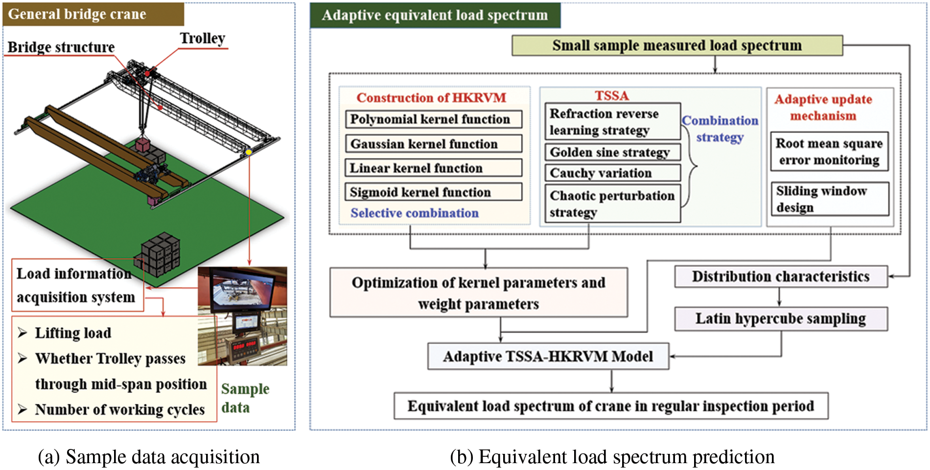
Figure 1: Equivalent load spectrum prediction model based on adaptive TSSA-HKRVM

As given in Fig. 1a, the load information acquisition system is employed to collect the sample data of load spectrum characteristic parameters, such as lifting load, whether the trolley passes through the mid-span position or not, and the corresponding number of working cycles. And the sample data are compiled into the measured load spectrum of small samples. The linear kernel function, polynomial kernel function, Gaussian kernel function, and sigmoid kernel function are adopted to examine the performance of single and mixed kernels. And the heterogeneous kernel RVM (HKRVM) model with complete expression capabilities is built on the complementary benefits of diverse kernel functions. The TSSA algorithm with global search ability is designed based on the SSA optimization algorithm by introducing the combination strategy of ‘refraction back learning, golden sine, and Cauchy variation + logistic chaotic perturbation’. And the optimization results of the relevant parameters of the HKRVM model are determined. The adaptive updating mechanism of the HKRVM model is defined by the sliding window design to create an adaptive TSSA-HKRVM model from the standpoint of ‘prediction + monitoring’. In line with the distribution characteristics of sample data of load spectrum characteristic parameters, the equivalent load spectrum prediction of the crane under the regular inspection cycle is completed by LHS sampling and the trained TSSA-HKRVM model, as presented in Fig. 1b.

2.2 Construction of HKRVM

In the description of the crane load spectrum, the machine learning algorithm is an emerging technology to solve regression prediction problems at present, mainly including BP neural network, support vector machine (SVM), and correlation vector machine (RVM) [20]. RVM is a model for learning probabilities sparsely. Its generalization and approximation abilities for small sample data are greater than those of the BP neural network built on conventional statistical theory. In addition, while maintaining the properties of SVM, RVM gets around issues with estimating the penalty coefficient of SVM and the need for the kernel function to satisfy Mercer's theorem. It is easier to use and makes predictions more accurate [21]. In choosing the optimal RVM kernel function, as compared to the single kernel learning approach, the use of multiple kernel functions may prevent blind selection. And it allows for the simultaneous processing of the heterogeneous information present in the data and improves prediction performance [22].

RVM model defines that under the condition of the input vector x, the form of the conditional probability distribution p of target variable t is:

{p(t|x,ω,σ2)=N[f(x,ω),σ2]f(x,ω)=∑i=1nωigi(x)+ω0(1)

where N[f(x,ω),σ2] is the normal distribution function. f(x,ω) is the mapping function. σ2 is the variance of target variable t. gi(x) is the ith basis function, i = 1, 2, …, n. n is the number of base functions. ωi is the ith weight corresponding to gi(x). t follows the normal distribution with mean f(x,ω) and variance σ2.

RVM model has m independent input vector sets X={xj},(j=1,2,…,m) and corresponding target vectors T={tj}. The maximum likelihood function pml of T is:

pml(T)=Πj=1mp(tj|xj,ω,σ2)(2)

To solve the weight vector, the prior probability distribution with the mean value of 0 and variance of αi2 is introduced. The posterior probability of ωi can be obtained after inputting the vector set X and T. Through the maximum likelihood boundary, it is found that most of αi approach 0, that is, the corresponding basis function has no effect on the RVM model prediction, which is converted into a sparse model, greatly simplifying the prediction calculation. When the input vector of the RVM model is x∗, its predicted output is t∗, and the relationship between the two is:

{p(t∗)=N[σ−2TG∑Tg⌢(x∗),ζ2]ζ2=[m−∑i=1n+1(1−∑ii)][‖T−σ−2G∑GTT‖2]−1+g⌢(x∗)T∑g⌢(x∗)(3)

where ζ2 is the variance of predicted results of RVM model. ∑ is a covariance matrix, ∑=[diag(α1,α2,…,αi)+σ−2GTG]−1. diag(α1,α2,…,αi) is the diagonal matrix with diagonal element αi. G is the kernel function matrix, Gji=gi(xj), Gjn=1. g⌢(x)T=[1,g1(x),…,gn(x)]. ‖T−σ−2G∑GTT‖ is the modulus. t∗ obeys the normal distribution with mean σ−2TG∑Tg⌢(x∗) and variance ζ2. ∑ii is the diagonal elements of the covariance matrix.

In RVM, as a bridge from low-dimensional to high-dimensional space, the kernel function is the pivot of transforming the nonlinear relationship into the linear relationship, which is the critical link affecting its regression prediction performance. As described in [23], RVM is more relaxed in the selection of kernel functions, but some more basic kernel functions are often applied in practical applications, such as: linear kernel function KPoly, polynomial kernel function KPoly_n, Gaussian kernel function KGauss, and Sigmoid kernel function KSigmoid. For any kernel function, it has applicability and limitations. The linear kernel function is simple and efficient, only applicable to linear and low-degree nonlinear prediction. The Gaussian kernel function has strong nonlinear approximation and generalization ability, which takes a long time and has poor global characteristics. For the Sigmoid kernel function, the global performance is better. The parameters are limited, and the nonlinear fitting degree of the complex problem is lower. The polynomial kernel function has good global characteristics. But it has too many parameters and lower performance of nonlinear fitting. Therefore, in practical engineering applications, for the single kernel function, the limitation is obvious, the fitting accuracy is lower, and there are problems such as inappropriate selection of the best kernel function. Based on the kernel function theory, the multi-core model is designed, and several common kernel functions are complementary according to different characteristics of the kernel functions to construct heterogeneous kernel functions with comprehensive expression ability, as shown in Eq. (4).

{KPoly(xi,xj)=xi⋅xjTKPoly_n(xi,xj)=[(cxi⋅xjT)+1]dKGauss(xi,xj)=exp⁡(−‖xi−xjT‖/2σ2)σ>0KSigmoid(xi,xj)=tanh⁡(γxi⋅xjT+θ)γ>0,θ<0K~(xi,xj)=∑q=1zwqKq(xi,xj)(4)

where, c, d are the coefficients of the Polynomial function. σ is the width factor of the Gaussian function, which controls the scope of the function. γ and θ are the parameters of the Sigmoid function. z is the number of kernel functions, z=2,3,4. wq is the corresponding weight parameter and ∑q=1zwq=1,0≤wq≤1, q=1,2,…,z.

Based on the regression prediction theory of RVM (see Eqs. (1)~(3)) and following the heterogeneous principle of the kernel function (see Eq. (4)), the HKRVM with comprehensive expression ability is constructed by the test on the sample data of crane load spectrum. And Section 4.2.1 gives the results.

2.3 Optimization of Kernel Parameters and Weight Parameters

The type of kernel function and the value of the kernel parameter have an influence at different levels on the prediction performance of HKRVM. The kernel parameters determine the ability of kernel function mapping, which indirectly affects the prediction performance to a greater extent. The traditional generalized root means square method, subjective assignment method, cross-validation method, and gradient descent method all have problems, such as higher calculation cost, greater training error, and stronger human interference in the optimization of kernel parameters and weight parameters. Therefore, the combination strategy is introduced to improve the sparrow optimization algorithm (SSA [24]), thus forming the TSSA algorithm to automatically optimize the kernel and weight parameters. The prediction accuracy of the HKRVM model is improved and the influence of subjective factors and other random factors is eliminated effectively.

2.3.1 Basic Principles of SSA

SSA is a novel intelligent optimization algorithm that mimics sparrow hunting and anti-hunting operations. Discoverers, followers, and scouters are the population members. The basic principle is to abstract the foraging and anti-predation processes of sparrows, such as discoverers searching for food, followers joining foraging, and scouts deciding whether to change the safe area [25].

In SSA, the position of the sparrow population corresponds to the effective solution of the search space. The sparrow population position Xi and the fitness of all sparrows F(Xi) can be expressed as:

{Xi=[x1,…,xd]F(Xi)=[f(x1),f(x2),…,f(xd)](5)

where, i=1,…,n and n is the number of sparrow population. d is the spatial dimension. f(xi) is the fitness function.

When the energy reserve of the discoverer is higher, the corresponding fitness value of the individual is larger, and the updated equation is:

Xi,jt+1={Xi,jtexp⁡(−i/(α⋅Max_iter)),R2<STXi,jt+QL,R2≥ST(6)

where, t is the current iteration number. Max_iter is the maximum number of iterations. Xi,j is the position of the ith sparrow in j-dimensional space, and α is a random number. Q is a random number, satisfying the normal distribution. L is d-dimensional full 1 matrix. R2 is the position warning value 0≤R2≤1. ST is the position safety value, which meets 0.5≤ST≤1.

The remaining individuals of the sparrow population are followers, and the updated equation is:

Xi,jt+1={Xi,jexp⁡((Xworst−Xi,jt)/i2)i>n/2Xpt+1+|Xi,j−Xpt+1|A+Li≤n/2(7)

where, Xp is the global optimal location of the discoverer for iteration t+1. Xworst is the worst global location in the current iteration. A+=AT(AAT)−1 and A is the matrix with each element being randomly values 1 or −1.

For i>n/2, the ith follower is starving and is unable to eat enough food and it will fly to other secure locations for feeding. For i≤n/2, it indicates that the ith follower is an ordinary or competitive member. The competitive members serve as scouter to enable food competition and early warning, making up typically 10% to 20% of the whole population, while the ordinary members follow the followers to collect sufficient energy. The equation for updates is:

Xi,jt+1={Xbestt+1+β|Xi,jt−Xbestt|fi≠fgXpt+1+K(|Xi,jt−Xworstt|/((fi−fw)+ε))fi=fg(8)

where Xbest is the global optimal position. K is random step size, −1≤K≤1. β is the control parameter for step size, being the normal distribution. ε is a minimum constant. fi is the fitness value of the ith individual. fg is the optimal fitness value of the population. fw is the worst fitness value of the population.

For fi≠fg , the sparrow is on the edge of the sparrow population and is vulnerable to predators. For fi=fg, the individual in the inner part of the population is aware of the threat of predators and approaches the surrounding sparrows in time to avoid being attacked.

2.3.2 Combination Strategy of Improving SSA

Although SSA has a fast convergence speed and strong search ability, as a swarm intelligence optimization algorithm, its global search ability is poor, and it is easy to fall into local optimization. The following improvement strategies are introduced to overcome these disadvantages.

1) Refraction reverse learning strategy

For the refraction reverse learning strategy [26], the reverse solution is constructed through reverse learning to improve the quality and diversity of the population of SSA. Meanwhile, based on the reverse solution, the refraction theorem of light is introduced to reduce the probability of falling into the local extreme value.

Assuming that the current feasible solution is Xi=(x1,x2,…,xm), the current optimal solution is Xbesti=(x1best,x2best,…,xmbest). Using reverse learning, the reverse optimal solution is:

{Xbesti′(t)=b+r⋅(a−Xbesti)Xbesti=(a+b)/2+(a+b)/2λ−Xbest/λλ=2π(1−sinc[(Max_iter−t)2/Max_iter2])xi,jt+1=Xbest′(t)+r⊕[Xbest(t)−Xbest′(t)](9)

where, b and a are the upper and lower bounds of the search space. Xbesti′(t) is the reverse solution of the current optimal solution. λ is the scaling factor. r is the dynamic random coefficient, 0≤r≤1.

2) Golden sine strategy

In Eq. (6), the discoverer will walk randomly according to the normal distribution. This randomness affects the search trend of the entire population, resulting in poor optimization performance, slower convergence speed, and an increased probability of falling into the local optimum. The golden sine strategy [27] has the characteristics of good robustness and fast convergence. It can be introduced into the discoverer update formula, and the oscillation change characteristics of the sine model can be applied to the location change of the discoverer, thus improving the diversity of the discoverer population and increasing the optimization area. At the same time, the golden section number can reduce the search space and accelerate the convergence speed, to achieve a good balance between ‘local search’ and ‘global development’. The improved equation is as follows:

Xi,jt+1={Xi,jtexp⁡[−i/(αMax_iter)]R2<STXi,jt|sin⁡(C1)|+Rsin⁡(C2)(C3Xp−C4Xi,jt)R2≥ST(10)

where, C1 is the distance control parameter, 0≤C1≤2π. C2 is the direction control parameter, 0≤C2≤π. C3 is the golden section coefficient, C3=−π+2π(1−u). u is the number of golden sections, u=(5−1)/2. C4 is the golden section coefficient, C4=−π+2πu.

3) Cauchy variation + logistic chaotic perturbation strategy

In the algorithm iteration process of SSA, the early-stage deviates from the target value, and various local optimizations in the later stage are nearly invalid. The simple and high-sensitive logistic chaotic map [28] is adopted to adjust Cauchy perturbation [29], which gives full play to the fine performance of the original Cauchy perturbation and has good chaotic ergodicity. The improved formula is as follows:

Xi,jt+1=τXbest(t)+(1−τ)cauchy(0,1)⊕Xbest(t)(11)

where, cauchy(0,1) follows the typical Cauchy distribution. τ conforms to logistic chaotic mapping, τi+1=κτi(1−τi), taking κ=4. ⊕ is the operator.

The combination strategy of ‘refraction reverse learning, golden sine, and Cauchy variation + logistic chaotic perturbation’ is introduced to improve SSA, thus forming TSSA. With the kernel parameters and weight parameters as the design variables and the root mean square error of HKRVM prediction results as the objective function, the optimization of parameters is completed through TSSA within the range of corresponding parameter settings. On this basis, the TSSA-HKMRVM model is constructed to forecast the crane load spectrum.

2.4 Definition of Adaptive Mechanism

The existing crane load prediction methods based on machine learning all predict large samples with fixed small samples. The optimization of relevant parameters of the machine learning model is realized by an intelligent optimization algorithm, which reflects the adaptability of the model parameters. But the increase in prediction steps for the long-term prediction process makes it difficult to ensure prediction accuracy. The reason is the diversity, randomness, and uncertainty of the load of the general bridge crane in the working cycle. Under various working cycle processes (as shown in Fig. 2), the lifting load will change unpredictably, namely that its probability density function will also be inconsistent. Therefore, from the standpoint of ‘prediction + monitoring’, the sliding window design [30] is employed to provide an adaptive update mechanism of the TSSA-HKRVM prediction model. The particular implementation approach is presented in Fig. 3.

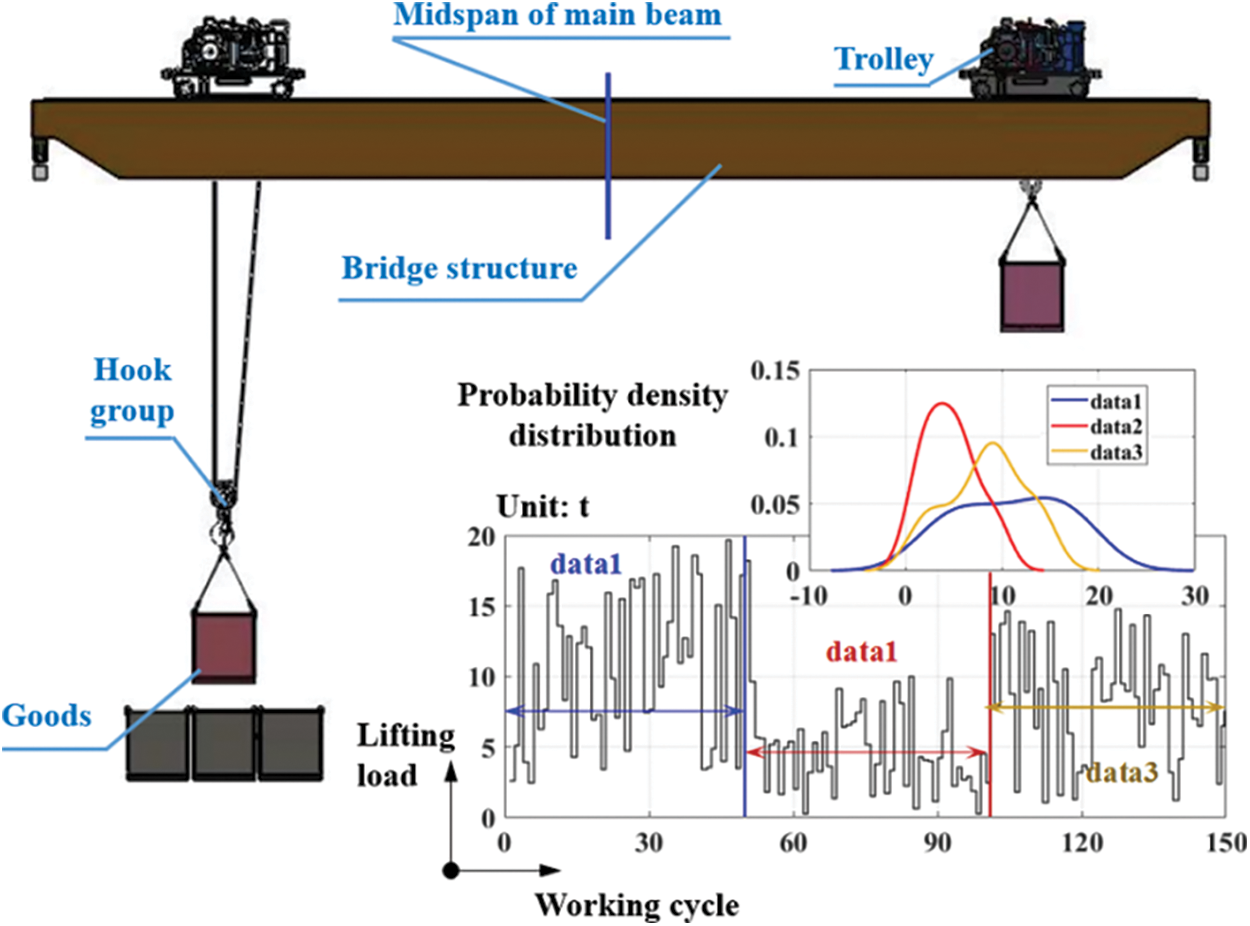
Figure 2: Load characteristic description

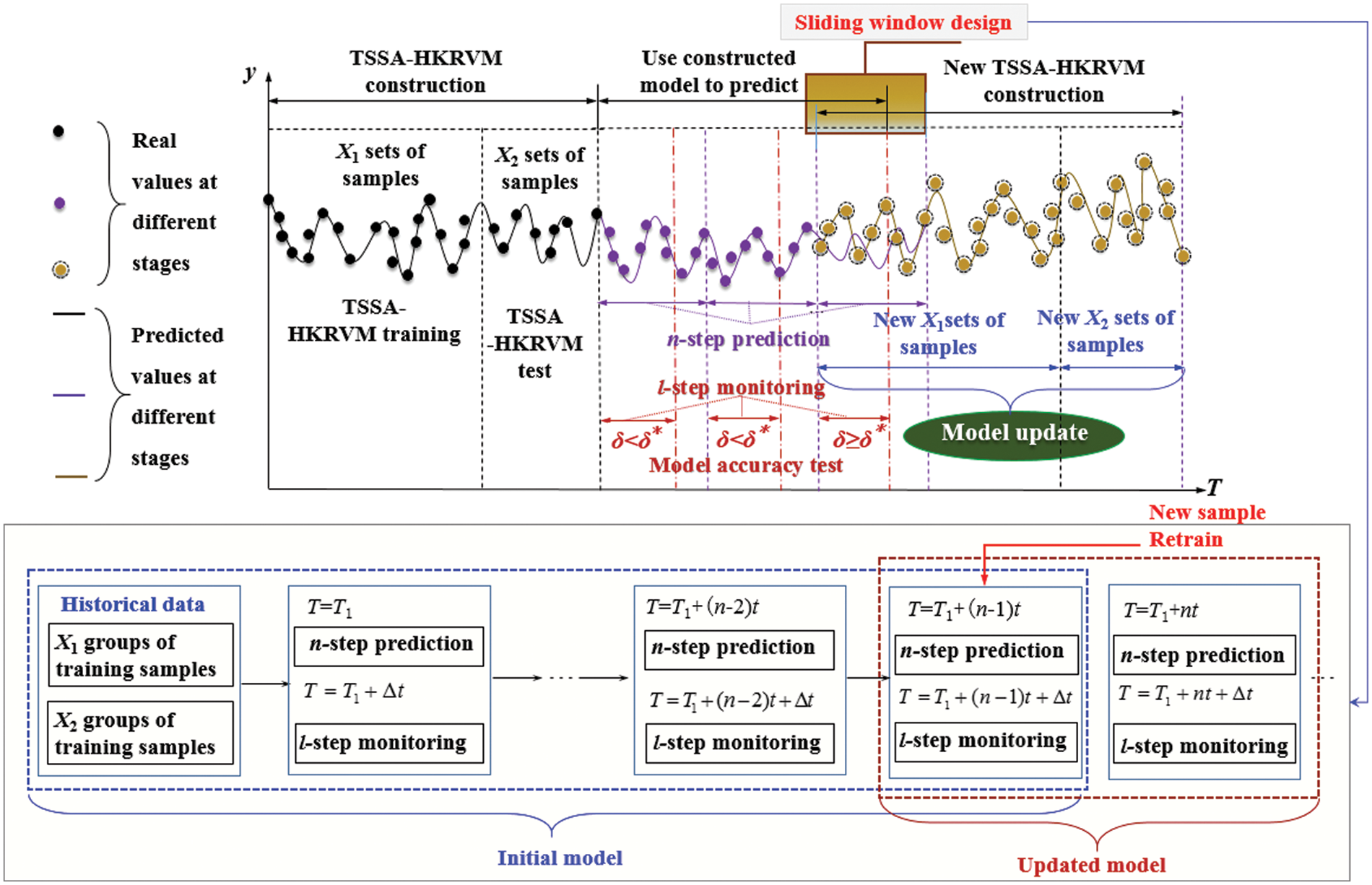
Figure 3: Adaptive update mechanism of prediction model

As illustrated in Fig. 3, the adaptive updating mechanism of the prediction model of the crane load spectrum includes three stages: ① TSSA-HKRVM construction, ② using the constructed model to predict, and ③ new TSSA-HKRVM construction.

In ① stage, the measured load spectrum of small samples is as the sample data set {(Xi,Yi)}i=1N. The total sample data is N = X1+X2, in which X1 groups are randomly selected for TSSA-HKRVM model training, and the remaining X2 groups are applied for model testing.

In ② stage, the TSSA-HKRVM model constructed in ① stage is employed to predict the n-step load spectrum, and the first l-step of n-step prediction is applied for monitoring, n≥l. In l-step monitoring, the root mean square test is performed on the prediction results to determine whether the test result δ is under the given constraint condition δ∗ (the threshold value set according to the actual load measurement accuracy requirements). For δ<δ∗, the model has good prediction performance and can continue to predict, by analogy, δ≥δ∗ appears for the first time in the kth n-step, indicating that continuous prediction will lead to significant errors.

In ③ stage, since δ≥δ∗ occurs in the kth n-step of ② stage, the sliding window design should be introduced at the end of the (k−1)th n-step, and the TSSA-HKRVM model should be re-established using the new sample data set {(Xi⌢,Yi⌢)}i=1N. So, the adaptive update of the TSSA-HKRVM model can be achieved by updating the measured samples of the load spectrum.

3  Implementation Process of Equivalent Load Prediction

The definition of crane load spectrum currently refers to the relationship between the load on the metal structure and the cumulative frequency of the load under the corresponding working cycle in the actual service process [31]. However, for general bridge cranes, one working cycle is a complete process from lifting one object on the ground to lifting the next, including the operation and regular stop of cranes and trolleys, as shown in Fig. 3. From the perspective of fatigue life, one of the critical parameters to judge whether the crane bridge structure can safely serve is the stress amplitude spectrum at the dangerous points of the structure during the working cycle. The main factors affecting the stress amplitude include the load size and the range of the loaded trolley movement. Namely, the damage to the bridge structure caused by the loaded trolley ‘passing through the middle of the main beam’ and ‘not passing through the middle of the main beam’ is different during the working cycle. Therefore, for the crane load spectrum, it is limited to only using the load size and the corresponding frequency to characterize.

Given this, through structural fatigue life analysis from the aspect of safe service of the crane bridge structure, in accordance with ‘GB/T30024-2020 cranes—proof of competence of steel structures’ [32] and in combination with the stress changes at dangerous points, it is determined that the characteristic parameters affecting the stress amplitude are ‘lifting load x1’, ‘whether the loaded trolley passes the mid-span position x2’ and the corresponding ‘number of working cycles y’. So, the relationship among x1, x2, and y is defined as the equivalent load spectrum.

Before forecasting the crane equivalent load spectrum under the periodic inspection cycle, the load information collection system has been built as shown in Fig. 4, according to the process of ‘collected objects→sensor layout→data acquisition→data processing→data presentation’ to obtain the characteristic parameter data of the load spectrum and compile it into the small samples measured load spectrum {x1i,x2i,yi}i=1N.

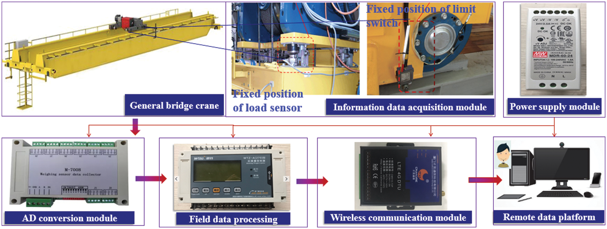
Figure 4: Crane load information acquisition system

As illustrated in Fig. 4, the crane load information acquisition system consists of a general bridge crane, information data acquisition module, AD conversion module, field data processing module, wireless communication module, remote data platform, and power supply module. 1) The information data acquisition module is composed of load sensors and cross-limiters. The load sensors are fixed at the drum support position of the crane trolley. The reading on the load sensor changing from 0 to 0 again corresponds to a complete working cycle of the crane. The load sensor measures the size of the current lifting load. The cross-limiters are installed near the left and right wheels of the trolley, the striker is mounted at the mid-span position of the main beam, and they are employed to record whether the trolley passes the mid-span section of the main beam in every working cycle. When the cross-limiter contacts the striker, it is recorded as 1, indicating that the loaded trolley passes the mid-span position. Otherwise, it is recorded as 0, implying that the loaded trolley does not go through the mid-span position. 2) The AD conversion module receives the low-level signals collected by each sensor, outputs them as digital signals, and transmits them to the field data processing instrument. 3) The field data processing module displays the collected data and sends it to the wireless communication module after completing the protocol conversion. 4) The wireless communication module transmits and stores the load information data to the remote data platform, and completes the collection of small sample load information clusters after data preprocessing. 5) The power supply module converts AC220V into DC24V and provides it to all instruments and modules on site.

Based on the measured load spectrum of the small sample {x1i,x2i,yi}i=1N, the TSSA-HKRVM model (Sections 2.2 and 2.3) and its adaptive update mechanism (Section 2.4) are utilized to predict the equivalent load spectrum of the general bridge crane under the regular inspection cycle (1 year) in combination with Latin hypercube sampling. The process is described in Fig. 5, and the specific steps are as follows:

1) Sample data without rigid quantification processing.

Normalize the small sample measured load spectrum {x1i,x2i,yi}i=1N, divide the processed sample into two parts, and randomly select group X1 as one part, and the remaining group X2 as the other part, so as to complete the data preparation.

2) TSSA-HKRVM construction, including HKRVM construction and parameter optimization.

Step 1. Based on the linear kernel function KPoly, polynomial kernel function KPoly_n, Gaussian kernel function KGauss, and Sigmoid kernel function KSigmoid, according to the characteristics of complementary advantages of kernel functions, mixed kernel functions are established by linear combination, and single and mixed kernel functions are tested with the prepared data to obtain the optimal kernel function, so as to complete the construction of HKRVM model and determine the required optimal kernel parameters and weight parameters.

Step 2. Initialization of population position and parameters of TSSA, such as population number N, maximum iterations Max_iter, error accuracy e, discoverer-follower ratio Rf and Rg, and safety value ST.

Step 3. According to the refraction reverse learning strategy (see Section 2.3.2, Part 1)), the initial position of the population members is modified by Eq. (9), and the fitness function is constructed through the root mean square error of the predicted results of the HKRVM model to calculate the fitness of the population individuals and determine the optimal individual position.

Step 4. Determine the number of discoverers, followers, and scouts in the population. According to the golden sine strategy (see Section 2.3.2, Part 2)), update the position of discoverers with Eq. (10), and update the positions of followers and scouts with Eqs. (7) and (8), respectively.

Step 5. Calculate the fitness of the individual population, determine the location of the best individual, and compare it with the fitness of the first five times. If the fitness does not change at this time, it is judged that it has fallen into the local optimum, and Step 6 is executed. If the fitness is optimal at this time, the iteration termination condition shall be judged. For the error accuracy or the maximum number of iterations meeting the requirements, output the specific values of the core parameters and weight parameters. For the iteration termination conditions being not met, execute Step 3.

Step 6. In case of falling into local optimum, Step 3 shall be executed after generating a new individual position with Eq. (11) according to Cauchy mutation and logistic chaotic perturbation strategy (see Section 2.3.2, Part 3).

3) Equivalent load spectrum prediction based on adaptive TSSA-HKRVM.

Step 1. The sample distribution information with ‘lifting load x1’ and ‘whether the trolley passes the mid-span position x2’ as the input variables are obtained by analyzing the sample data of the characteristic parameters of the load spectrum. According to the distribution characteristics, the input variables for the load spectrum to be predicted are generated through LHS sampling. And the trained TSSA-HKRVM model is used to predict the equivalent load spectrum.

Step 2. The accuracy of prediction results is checked by the root mean square error. For δ<δ∗, the prediction results are feasible, and the equivalent load spectrum under the regular inspection cycle is given through the inverse normalization processing. Otherwise, execute Step 2.

Step 3. For δ≥δ∗, according to the adaptive updating mechanism of the prediction model (see Section 2.4), update the small sample measured load spectrum of and execute 1), analogously, to complete the prediction of the equivalent load spectrum of the crane under each periodic inspection cycle.

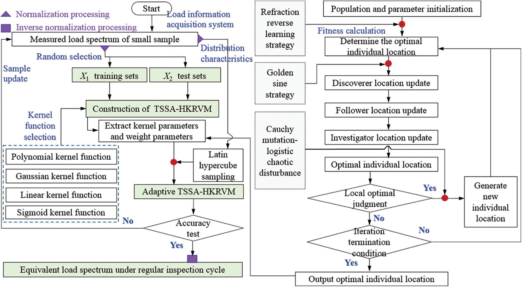
Figure 5: Flow chart of crane equivalent load spectrum

4  Engineering Examples

Taking the QD20/10 t × 43 m × 12 m general bridge crane as the research object, the equivalent load spectrum prediction of the crane under the regular inspection cycle (one year) is completed by the above method.

4.1 Equivalent Load Spectrum under Regular Inspection Cycle

Using the crane load information acquisition system (see Fig. 4), the 60-day working processes of the crane in an enterprise are tracked in real-time. ‘lifting load x1’ and ‘whether the trolley passes through the mid-span position or not x2’ is taken as the input variables, that is, the characteristic parameters of the load spectrum. And taking the number of working cycles as the feedback object, the small sample measured load spectrum is compiled, as shown in Table 1. The heterogeneous kernel function is composed of KGauss and KPoly_n, the reason is given in Section 4.2.1. The kernel parameters σ, d, c and the weight parameters w1,w2 are determined.

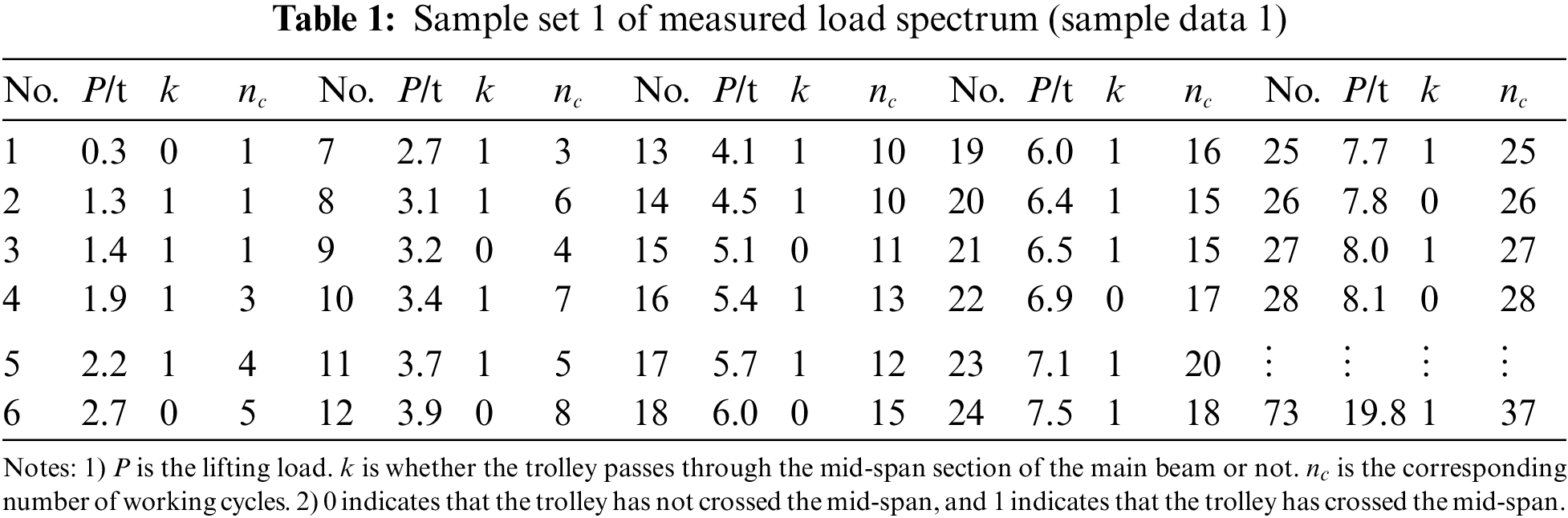
After normalizing the data in Table 1, 58 groups of samples are randomly selected to complete the TSSA-HKRVM model training, and the remaining 15 groups are utilized for the model testing. The initial parameters of the model are as follows: the population number of TSSA is 20, the maximum number of iterations N is 100, the error accuracy e is 0.1, the ratio values Rf and Rg of the discoverer and the follower are 0.7 and 0.2, and the safety ST is 0.6. After the relevant parameters are set, the model is repeatedly trained for 20 times to obtain the mean value of the kernel parameters {σ,d,α}={0.096,0.121,0.1208} and the mean value of the weight parameters {w1,w2}={0.1235,0.8765} to form TSSA-HKRVM(0.096,0.121,0.1208,0.1235,0.8765). The relevant test results are shown in Fig. 6.

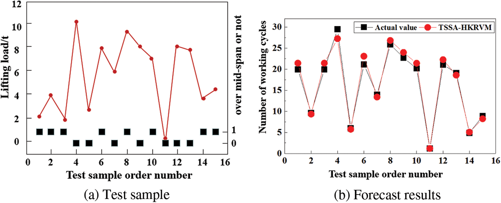
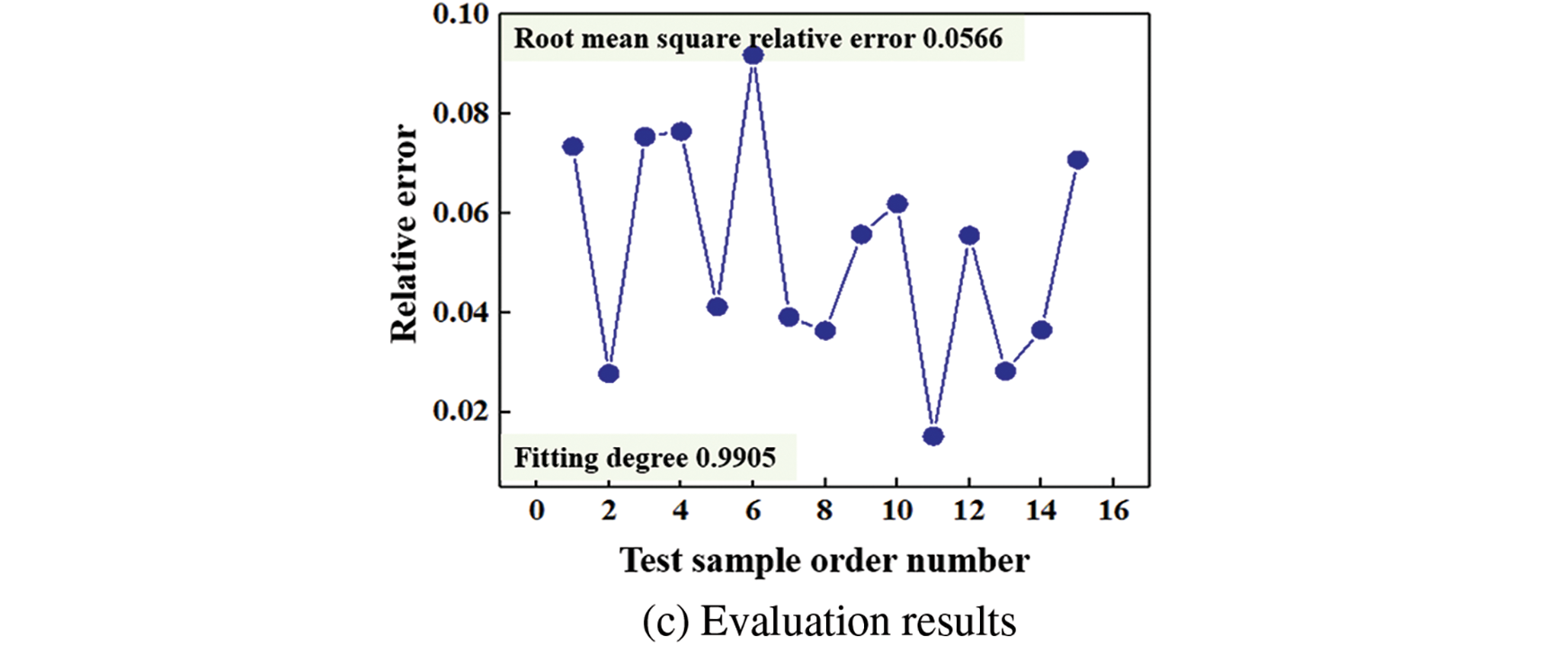
Figure 6: Test results of TSSA-HKRVM

It can be seen from Fig. 6 that, based on the trained TSSA-HKRVM(0.096,0.121,0.1208,0.1235, 0.8765) model, 15 groups of test samples are used to test the model. The maximum relative error between the predicted result and the real value is 0.0918, the root mean square relative error is 0.0566, and the goodness of fit is 0.9905.

The distribution of each input variable is obtained by analyzing the data in Table 1. The ‘lifting load’ meets the uniform distribution X∼U(0.6,19.9), and ‘whether the trolley passes through the mid-span position or not x2’ meets the 0–1 distribution X∼B(x,0.6933). After inverse normalization, the prediction results of the number of corresponding working cycles y can be obtained by combining LHS sampling with the trained TSSA-HKRVM model, taking 10-steps as the prediction cycle and 5-steps as the monitoring cycle (set the root mean square relative error threshold δ∗=0.1), as shown in Fig. 7.

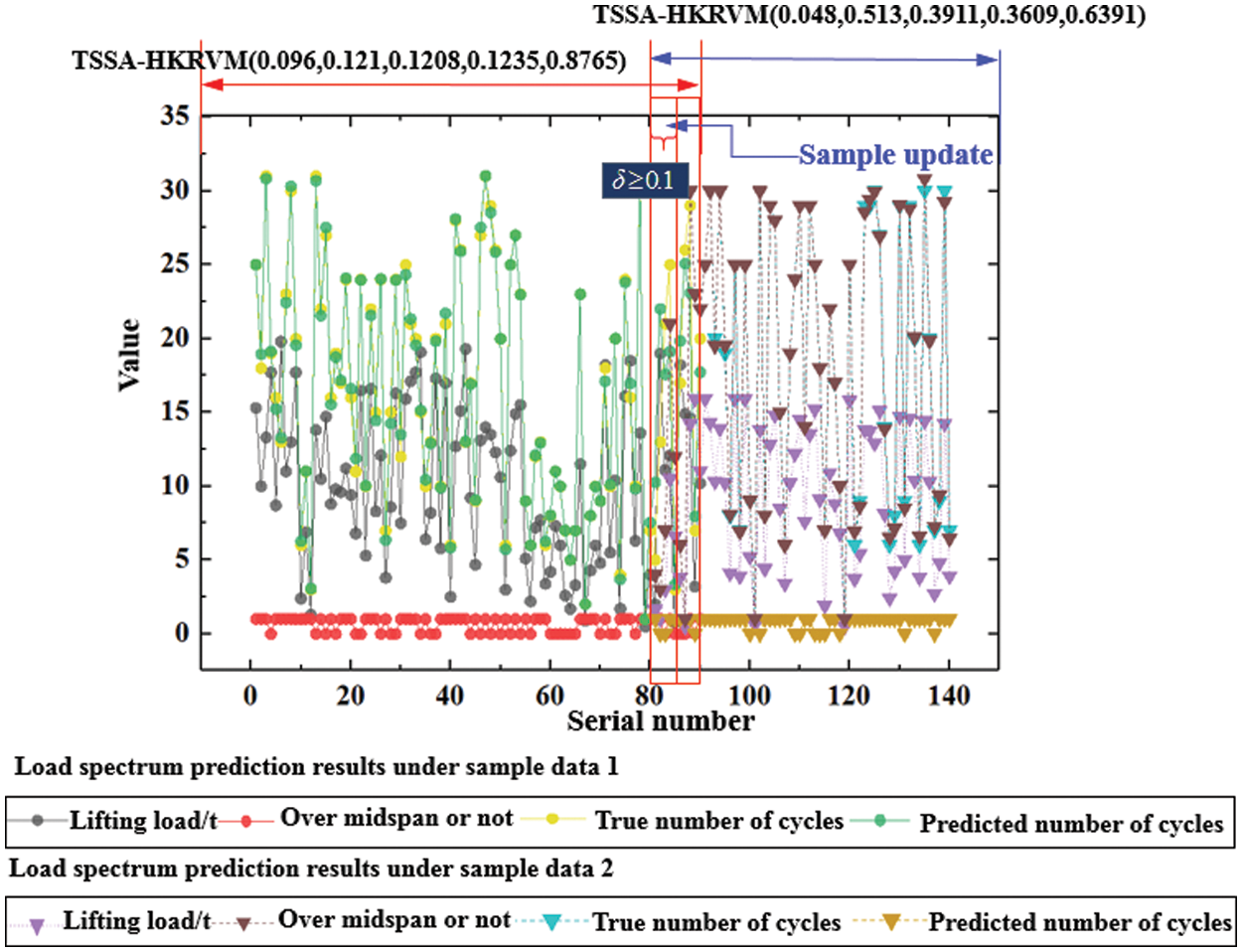
Figure 7: Prediction results of TSSA-HKRVM under adaptive update

It can be seen from Fig. 7 that based on the TSSA-HKRVM(0.096,0.121,0.1208,0.1235,0.8765) model trained and tested by sample data 1. When the prediction steps reach 80~85, the root mean square relative error of the prediction results under the monitoring cycle is δ=0.178>δ∗(0.1). At this time, at the end of the 8th prediction cycle, the adaptive update mechanism is adopted (see Section 2.4). Combined with data sample 2 (see Table 2), the TSSA-HKRVM is retrained and tested, and a new TSSA-HKRVM(0.048,0.513,0.3911,0.3609,0.6391) model is determined. By analogy, the equivalent load spectrum of the QD20/10 t–43 m general bridge crane is obtained under the regular inspection cycle, as shown in Fig. 8. The load spectrum for the subsequent regular inspection cycles is determined in the similar way, which will not be repeated here.

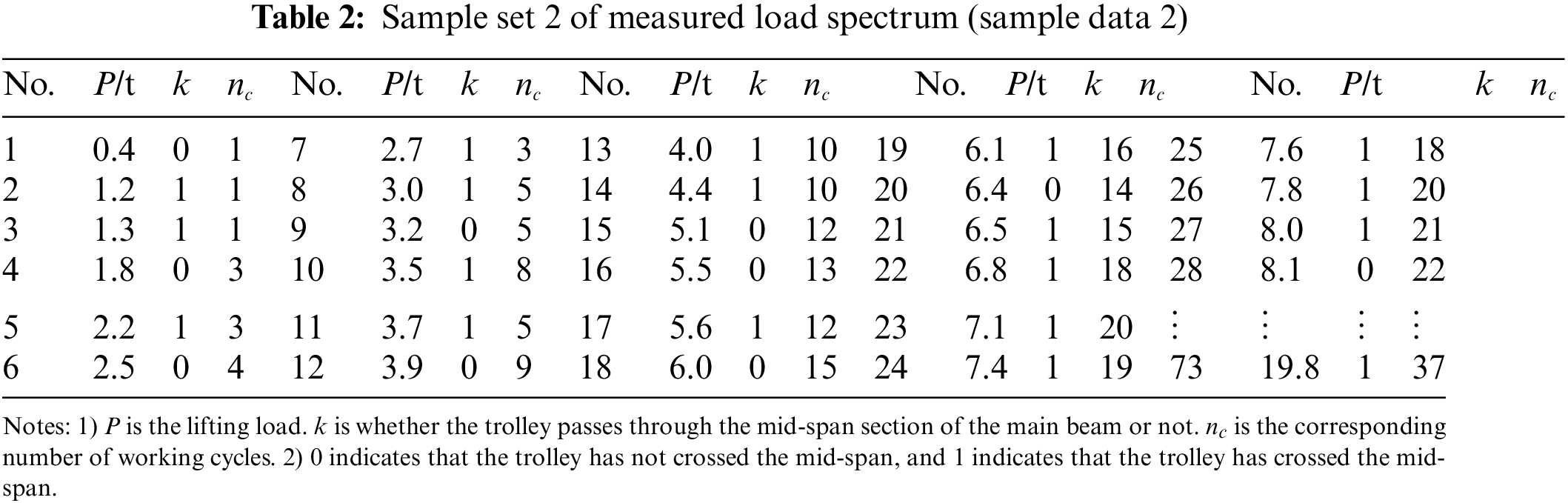
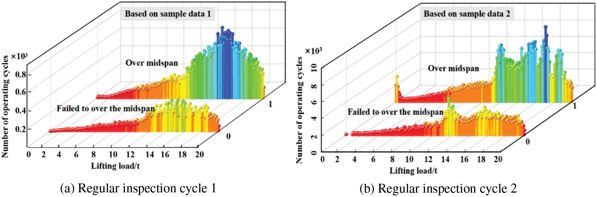
Figure 8: Equivalent load spectrum under regular inspection cycle

4.2 Result Analysis and Discussion

The applicability of the method proposed in this paper is verified by discussing the influence of various influencing factors on the prediction results from four aspects, including the construction of kernel function, optimization of kernel parameters and weight parameters, adaptive control methods, and load spectrum prediction methods.

4.2.1 Construction of Kernel Function

To demonstrate the reasonableness of the selection of kernel function of the TSSA-HKRVM model, a single kernel function, two heterogeneous kernel functions and three heterogeneous kernel functions are contrasted and studied. The uniformity of the comparison test is considered and the TSSA algorithm is employed for relevant parameter optimization of any kernel function. The data in Table 2 are taken as samples. Among them, 58 groups of samples are randomly selected for the training of the TSSA-HKRVM model, and the remaining 15 groups are used for model testing. On this basis, the influence of the above kernel functions on the load spectrum prediction results is quantitatively analyzed and discussed. The relevant results are given in Fig. 9 and Table 3.

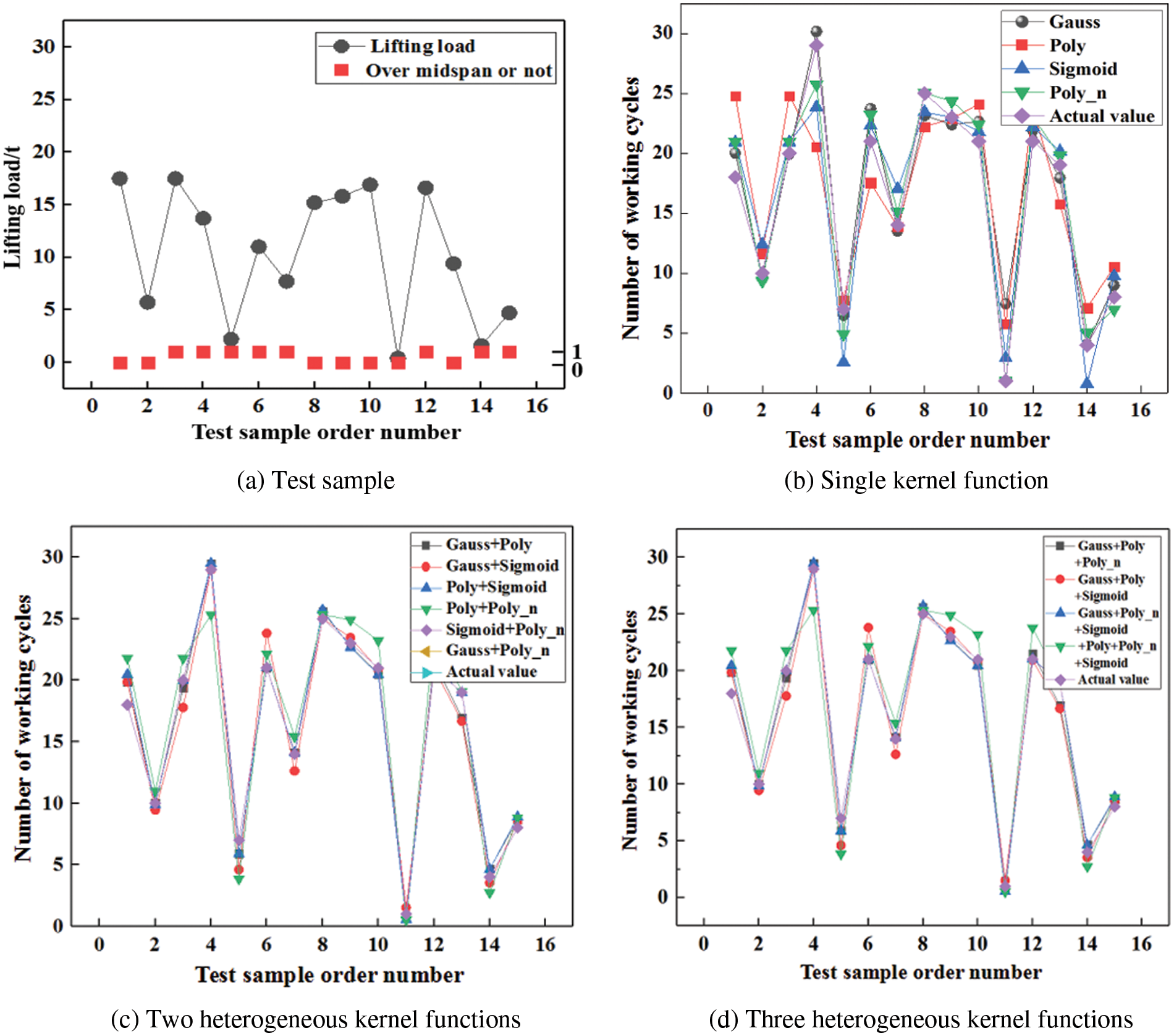
Figure 9: Prediction effect of TSSA-HKRVM under various kernel functions

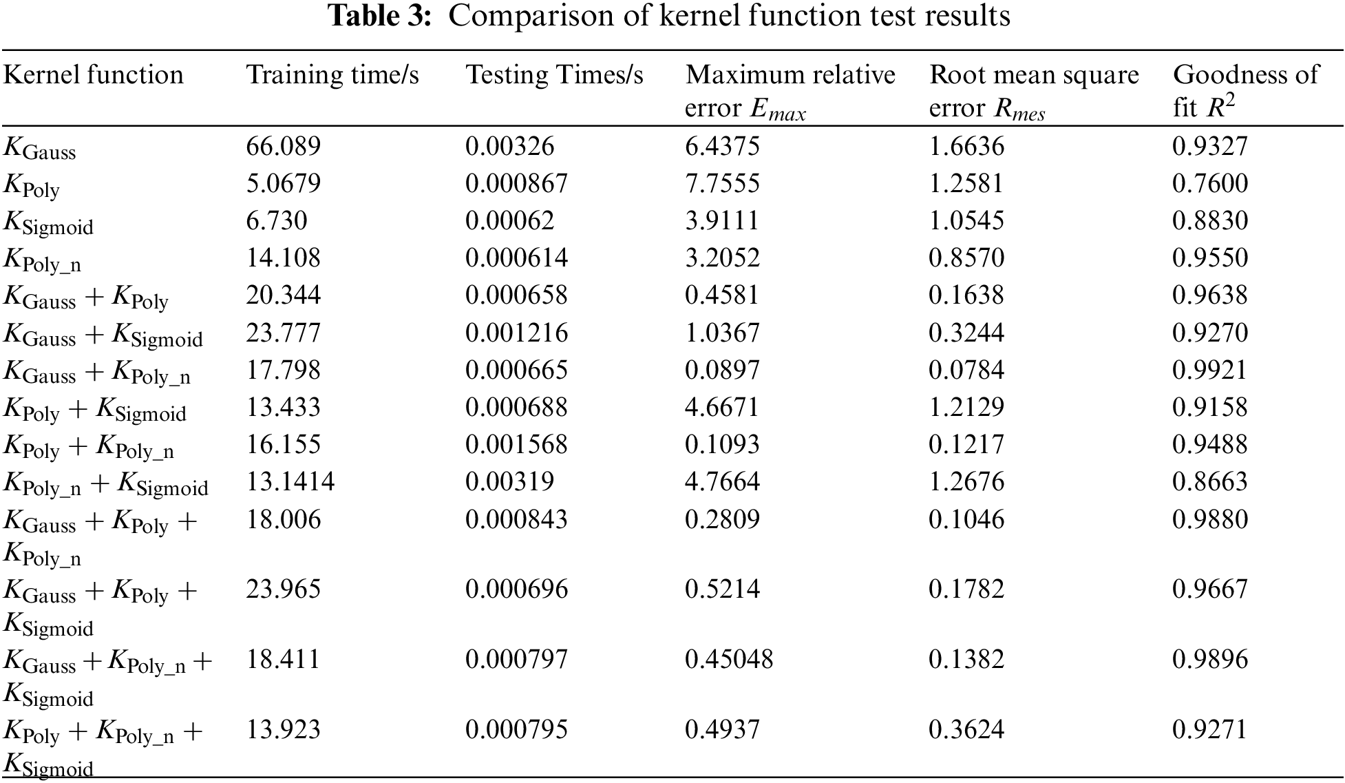
It can be seen from Fig. 9 and Table 3 that:

1) For a single kernel function, the results for the goodness of fit of KPoly_n and KGauss are higher and remain above 0.93. Due to the complex operation of KGauss, the training time of the model is longer. The operation costs of KSigmoid and KPoly are smaller, and the accuracies of the models are lower, which do not reach 0.9. Because of the limited value of parameters of KSigmoid, there are relatively few practical applications.

2) For the binomial heterogeneous kernel functions, the model accuracies have been significantly improved. For the heterogeneous combination of KPoly_n and KGauss, the fitting accuracy is controlled above 0.99, and the root mean square error is within 0.1. The prediction accuracy and error deviation of the model are better than the other two heterogeneous kernel functions, and the model operation efficiency is higher than the original KGauss model. It has the comprehensive expression ability of the KPoly_n model and the KGauss model.

3) For the trinomial heterogeneous kernel functions, the increase in the number of kernel functions leads to an increase in the model complexity. The fitting performance after mixing is considerably enhanced when compared to the original single kernel function, but not when compared to the two heterogeneous kernel functions.

To sum up, the heterogeneous kernel function benefits from diverse kernel functions, higher learning capacity, and better promotion ability. Considering the complexity, fitting degree, and calculation efficiency of the model comprehensively, the heterogeneous kernel function composed of KGauss and KPoly_n is selected to be the best in load spectrum prediction effect.

4.2.2 Acquisition Methods of Kernel Parameters and Weight Parameters

The effectiveness of the TSSA algorithm in parameter optimization of the HKRVM prediction model is verified by comparing TSSA with SSA, ISSA1 (the refraction inversion improved SSA), ISSA2 (the refraction inversion + golden sine hybrid improved SSA), ISSA3 (the refraction direction + golden sine + Cauchy strategy hybrid improved SSA).

The initial parameter settings are consistent, and the prediction model is HKRVM. On this basis and in combination with sample data 2 (Table 2), the influence of the above parameter acquisition methods (SSA-HKRVM, ISSA1-HKRVM, ISSA2-HKRVM, ISSA3-HKRVM, and TSSA- HKRVM) on the load spectrum prediction results is analyzed. The relevant results are shown in Fig. 10 and Table 4.

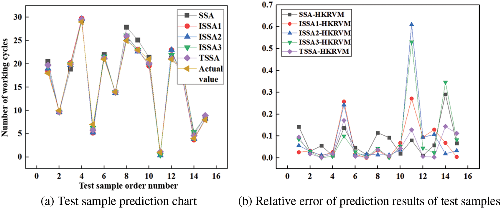
Figure 10: Prediction effect of HKRVM model based on different optimization algorithms

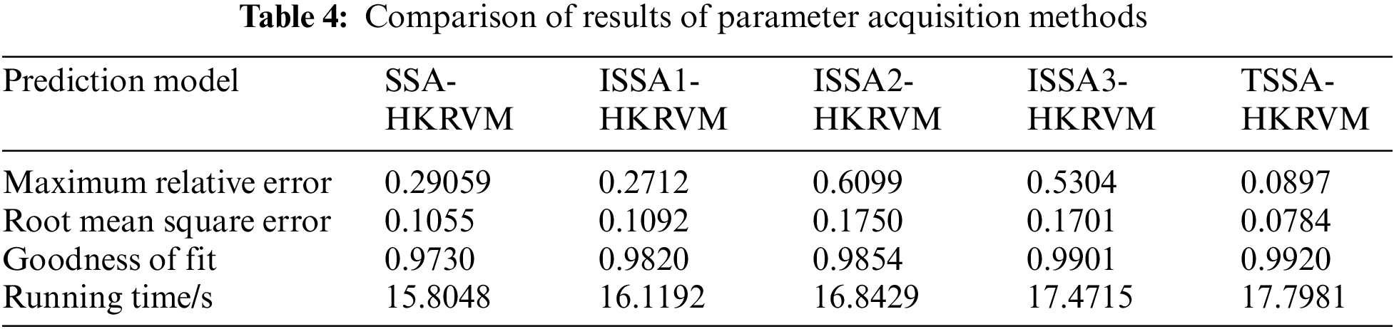
As can be seen from Fig. 10 and Table 4, the prediction abilities of ISSA1-HKRVM, ISSA2-HKRVM, ISSA3-HKRVM, and TSSA-HKRVM models have been significantly improved by the comparing with the SSA-HKRVM model. And the prediction accuracy, dispersion, and offset of the TSSA-HKRVM model are the best. The TSSA-HKRVM algorithm has a slight decrease in computational efficiency due to its high structural complexity, but its convergence speed and accuracy have been significantly improved. For sample data 2, the single optimization running times of SSA-HKRVM, ISSA1-HKRVM, ISSA2-HKRVM, ISSA3-HKRVM, and TSSA-HKRVM are 15.8048, 16.1192, 16.8429, 17.4715, and 17.7981 s, respectively. Compared with the parameter optimization of the TSSA-HKRVM model, the running time of ISSA2-HKRVM and ISSA3-HKRVM decreases by 5.3% and 1.83%, but the model dispersion increases by 1.23 times and 1.16 times. It can be seen that TSSA method is more excellent in parameter optimization of the HKRVM model.

4.2.3 Adaptive Control Methods

The feasibility of the adaptive mechanism proposed in this paper is validated in the prediction of the equivalent load spectrum of general bridge cranes by comparing it with the traditional adaptive predictive control methods [33,34], such as the adaptive predictive control method based on neural network [35] and the generalized predictive adaptive control algorithm [36]. For ‘whether the trolley passes through the mid-span position or not x2’, it is processed according to the 0–1 distribution. And only the case of the load is considered here. The neural network NNI hierarchy is 2–5–1, taking load samples under 3000 working cycles (one year) and learning 5000 times offline. The relative error of the root means square is less than 0.1. The forgetting factor of online training is 0.99. In the implicit generalized predictive control algorithm. The prediction length is 10, the control length is 10, the control weighting coefficient is 0.98, the softening coefficient is 0.4, the forgetting factor in the least squares parameter estimation is 0.98, and the matrix is 105I. The load prediction control process is described in Fig. 11.

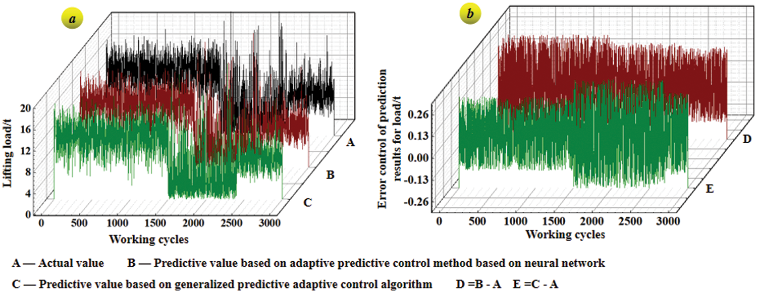
Figure 11: Load curve under working cycle based on adaptive control method

In the load prediction control curve in Fig. 11, mathematical statistics technology is employed to transform the curves into 80 groups of loads and their corresponding frequencies, namely 80 groups of load spectrums based on the two traditional adaptive predictive control methods. And the 80 groups of load spectra based on the TSSA-HKRVM model are given. The relevant results are given in Fig. 12.

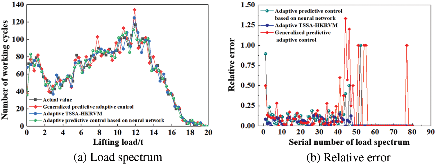
Figure 12: Load spectrum based on adaptive control methods

In Figs. 11 and 12, for the prediction method based on adaptive TSSA-HKRVM, the number of equivalent load spectra with a relative error of more than 10% within one year of the regular inspection cycle is 5, the relative error of root mean square is 0.0577, and the goodness of fit is 0.9895. For the adaptive predictive control algorithm based on neural network, the number of results with relative error exceeding 10% is 11, the root mean square relative error is 0.1883, and the goodness of fit is 0.9775. For the implicit generalized predictive control algorithm, the number of results with a relative error of more than 10% is 18, the root mean square relative error is 0.4172, and the goodness of fit is 0.9663.

The reason for the above phenomenon is that:

1) The predictive control method based on neural network is composed of neural unit adaptive PID controller and Smith predictor based on neural network. The predictor performs multi-step prediction on the output. And the controller acts ahead to eliminate the impact of time delay on the system. The adaptive PID controller realizes its weight adjustment through the supervised Hebb learning algorithm, and the adaptive control is achieved through the online adjustment of the weight coefficient. The degree of nonlinearity is good, and the robustness is high. However, there is no uniform standard for the selection of the neural network hierarchy. The designer makes a tentative choice according to his own experience. The subjective interference factors are stronger, and the prediction efficiency and accuracy are greatly affected by the network hierarchy.

2) The implicit generalized predictive control (IGPC) algorithm does not need to identify the model parameters of the object. And it uses input/output data to directly identify the controller parameters to solve the optimal control increment, which has the characteristics of small computation and high real-time performance. But its degree of nonlinear description is poor.

3) TSSA-HKRVM is based on small measured samples, directly controlling the prediction of load spectrum rather than the traditional control of the load change process. It is combined with the TSSA algorithm to carry out rolling optimization of relevant parameters of HKRVM. It uses the sliding window design and the sample update to carry out adaptive feedback correction from the perspective of ‘prediction + monitoring’. The load information is complete and the method has strong robustness, high prediction accuracy, and strong adaptive ability.

4.2.4 Load Spectrum Prediction Methods

The adaptive TSSA-HKRVM in the equivalent load spectrum prediction of general bridge cranes is demonstrated by comparing the method in the paper with the current swarm intelligence optimization algorithm improved relevance vector machine prediction technology (ILON-RVM [37]) and the LSSVM model (IBAS-LSSVM [16]) of crane load spectrum regression prediction.

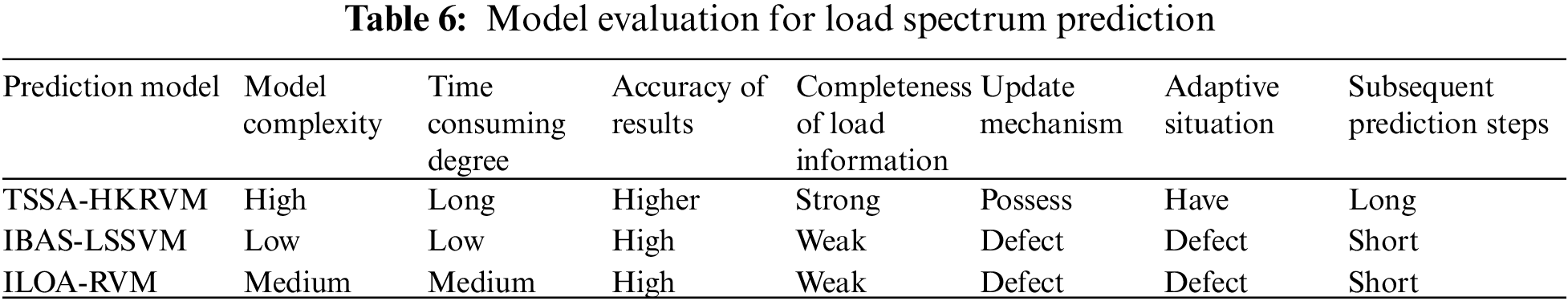
Table 5 displays the parameter settings for each model, and Table 2 lists all the samples. Following the completion of the setup, 58 sets of samples are randomly selected from the total sample number as training samples. The remaining 15 sets of samples are used as test samples to verify the prediction accuracy of the model. The training and testing phases of each prediction model are performed 20 times separately to confirm the stability and dependability of the training results. The average results for the goodness of fit of each prediction model are then determined. On this basis, the advantages and disadvantages of the above models are qualitatively discussed in the prediction of crane load spectrum. Relevant results are shown in Fig. 13 and Table 6.

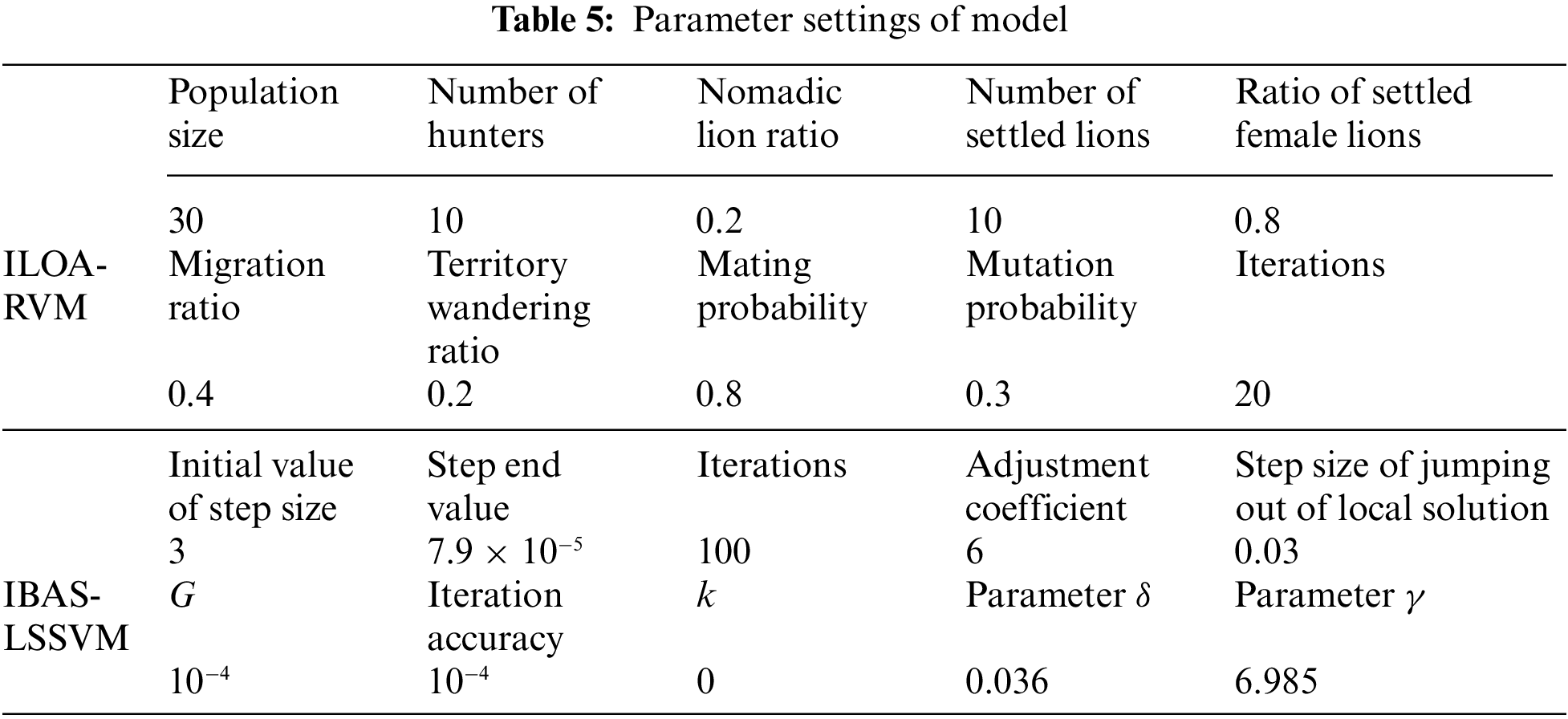
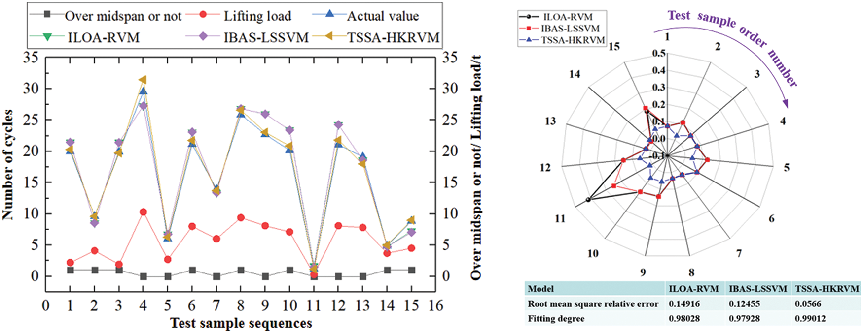
Figure 13: Test results of different prediction models

It can be seen from Fig. 13 that for ILOA-RVM, IBAS-LSSVM, and TSSA-HKRVM prediction models, the number of relative errors exceeding 10% is 7, 6 and 0. The root means square errors are 0.14916, 0.12455, and 0.0566. The results for the goodness of fit are all in the range of 0.979~0.983.

According to Table 6, IBAS-LSSVM uses the least square method to transform the non-equality constraints in the quadratic programming optimization problem of SVM into equality constraints for solving linear equations and takes the sum of squares of errors as the loss function of training samples, which reduces the complexity of sample points in the training process, but its kernel function must meet Mercer’s theorem. However, ILOA-RVM overcomes the issue that the specified kernel function must meet the Mercer criterion. It gives logistic chaotic mapping principles and advances the dynamic search interval approach, which makes the original lion individual more random and ergodic after chaotic transformation. It eliminates the drawbacks generated by the changeable length of the search interval. Compared with ILOA-RVM and IBAS-LSSVM, TSSA-HKRVM has the highest model complexity, longest time consumption, and the greatest prediction accuracy. The causes are as follows: from the angle of ‘prediction + monitoring’, TSSA-HKRVM uses the sliding window design to provide an adaptive update mechanism of the prediction model through sample updating. The load information is relatively complete. It addresses the problem that ILOA-RVM and IBAS-LSSVM forecast huge samples with fixed small samples, resulting in low accuracy in the process of long-term prediction.

5  Conclusions

An adaptive TSSA-HKRVM model for the regression prediction of crane load spectrum is proposed in the paper. It overcomes the problem that the randomness of the crane working load leads to the reduction of load spectrum prediction accuracy over time, which provides a basis for the compilation of load spectrum for crane matching design and retirement mechanism. The specific conclusions are as follows:

1) For the adaptive TSSA-HKRVM prediction model, single and mixed kernel functions are tested with load spectrum samples based on RVM to obtain the optimal combination of the heterogeneous kernel function (KPoly_n+KSigmoid). By making full use of the complementary advantages of different kernel functions, the prediction performance of the model is improved, thus overcoming the limitation of single kernel function and increasing the multi-core heterogeneous computing efficiency. A strategy consisting of ‘refraction reverse learning, golden sine, and Cauchy mutation + logistic chaotic perturbation’ is introduced into the SSA algorithm to form TSSA. And it overcomes the sensitivity of the manual setting of core parameters and weight parameters and improves the global search ability of the algorithm in each time domain during parameter rolling optimization. Through the way of ‘prediction + monitoring’, the adaptive updating mechanism of the model is given by the sliding window design, which also ensures the adaptability of the load prediction model throughout the life cycle of the crane.

2) The proposed method is applied to QD20/10 t × 43 m × 12 m general bridge crane. The results show that: compared with the traditional adaptive predictive control method, when the load samples are based on 3000 working cycles (one-year regular inspection cycle), the TSSA-HKRVM prediction has a higher fitting degree, a smaller root mean square error and higher predictive control performance of the model. Compared with the existing load spectrum prediction methods (ILOA-RVM and IBAS-LSSVM), TSSA-HKRVM has a higher model complexity, but it provides an adaptive update mechanism of the prediction model by updating samples, which improves the prediction accuracy of long periods, ensures the completeness of load information throughout the life cycle of the crane and has strong applicability and popularization.

Funding Statement: This paper is based on the extensive investigation and testing results finished by experts and testers from Zhuzhou Tianqiao Crane Co., Ltd., and Weite Technologies Co., Ltd. The author cordially thanks experts and testers for on-site survey and real-time detection. This paper is sponsored by the National Natural Science Foundation of China (52105269).

Conflicts of Interest: The authors declare that they have no conflicts of interest to report regarding the present study.

References

1. Zhou, J. C. (2021). Current situation and future of hoisting machinery industry. Construction Machinery, (1), 24–25. [Google Scholar]
2. Zhao, C. H. (2018). China is taking the lead in formulating four international standards for hoisting machinery. Hoisting and Conveying Machinery, 519(5), 34. [Google Scholar]
3. Teng, H. L., Li, B. W., Wei, X. (2020). Research on load spectrum of turboshaft engine based on main state recognition. Journal of Ordnance Equipment Engineering, 41(5), 144–150. [Google Scholar]
4. Liu, X. T., Wang, H. J., Wu, Q., Wang, Y. S. (2022). Uncertainty-based analysis of random load signal and fatigue life for mechanical structures. Archives of Computational Methods in Engineering, 29, 375–395. https://doi.org/10.1007/s11831-021-09579-6 [Google Scholar] [CrossRef]
5. Li, G. F., Wang, S. X., He, J. L., Wu, K. (2019). Compilation of load spectrum of machining center spindle and application in fatigue life prediction. Journal of Mechanical Science and Technology, 33(5), 1603–1613. https://doi.org/10.1007/s12206-019-0312-3 [Google Scholar] [CrossRef]
6. Ma, M. Z., Liu, X. T. (2022). Multiaxial fatigue life prediction for metallic materials considering loading path and additional hardening effect. International Journal of Structural Integrity, 13(3), 534–563. https://doi.org/10.1108/IJSI-03-2022-0023 [Google Scholar] [CrossRef]
7. Zou, X. H., Gou, L. L., Fu, L. (2022). Research on fatigue life of all-terrain vehicle control arm based on measured load spectrum. Journal of Ordnance Equipment Engineering, 43(7), 301–308. https://doi.org/10.12688/cobot [Google Scholar] [CrossRef]
8. Yan, T. H., Wang, W. G., Zhao, H. F. (2021). Development of structure monitoring systems and digital twin technology of active jacket platforms. China Mechanical Engineering, 32(20), 2508–2513. [Google Scholar]
9. Wong, L., Rathnayaka, S., Chiu, W. K. (2018). Utilising hydraulic transient excitation for fatigue crack monitoring of a cast iron pipeline using optical distributed sensing. Structural Control & Health Monitoring, 25(4), 16–23. https://doi.org/10.1002/stc.2141 [Google Scholar] [CrossRef]
10. Liu, J., Dai, H. Y., Song, Y. (2020). Test technology research and fatigue damage prediction of a car body based on dynamic simulation load spectrum. Journal of Zhejiang University Science, 21(11), 923–937. https://doi.org/10.1631/jzus.A1900662 [Google Scholar] [CrossRef]
11. Sun, Z. G., Xing, G. P., Song, Y. D. (2016). Simulation of multi-parameter random correlation load spectrum based on principal component analysis. CN105760610A. [Google Scholar]
12. Ge, W. T., Duan, L. Y., Yu, X. Z. (2019). A method of generating load spectrum data for dynamic load simulation. CN110069875A. [Google Scholar]
13. Dong, Q., Xu, G. N. (2017). Crane equivalent load spectrum prediction method based on relevance vector machine improved by adaptive double layer fruit fly algorithm. Journal of Machine Design, 34(2), 86–93. [Google Scholar]
14. Zuo, S. (2021). Fatigue life assessment of tower crane based on neural network to obtain stress spectrum (MA. Thesis). Taiyuan University of Science and Technology, Taiyuan, China. [Google Scholar]
15. Wang, S., Li, D. Y., Jiang, X. X. (2018). Development and application of crane load spectrum prediction software based on v-SVRM model. Modern Manufacturing Technology and Equipment, (11), 93–96. [Google Scholar]
16. Yu, Y. N., Qi, Q. S., Dong, Q., Xu, G. N. (2022). A study on optimization of the LSSVM model for crane load spectrum regression prediction. Journal of Vibration and Shock, 41(12), 215–228. [Google Scholar]
17. Pl, A. Fei, D., B., Gang, H. (2022). Machine learning-enabled estimation of crosswind load effect on tall buildings. Journal of Wind Engineering and Industrial Aerodynamics, 220, 1–16. [Google Scholar]
18. Zhao, J., Zhang, H. X., Zou, H. L. (2022). Probability prediction method of transmission line icing fault based on adaptive relevance vector machine. Energy Reports, 8(4), 1568–1577. https://doi.org/10.1016/j.egyr.2022.02.018 [Google Scholar] [CrossRef]
19. Qiao, W., Huang, K., Azimi, M. (2019). A novel hybrid prediction model for hourly gas consumption in supply side based on improved whale optimization algorithm and relevance vector machine. IEEE Access, 7, 88218–88230. https://doi.org/10.1109/ACCESS.2019.2918156 [Google Scholar] [CrossRef]
20. Liu, B., He, J. R., Geng, Y. J., Wang, Z. (2017). Recent advances in infrastructure architecture of parallel machine learning algorithms. Computer Engineering and Applications, 53(11), 31–38+89. [Google Scholar]
21. Acosta, S. M., Amoroso, A. L., Santanna, A., Junior, O. C. (2021). Relevance vector machine with tuning based on self-adaptive differential evolution approach for predictive modelling of a chemical process. Applied Mathematical Modelling, 95, 125–142. https://doi.org/10.1016/j.apm.2021.01.057 [Google Scholar] [CrossRef]
22. Wei, G., Mao, H. (2022). An optimal relevance vector machine with a modified degradation model for remaining useful lifetime prediction of lithium-ion batteries. Applied Soft Computing, 124, 108967. https://doi.org/10.1016/j.asoc.2022.108967 [Google Scholar] [CrossRef]
23. Liu, F. Y., Wang, S. H., Zhang, Y. D. (2018). Overview on models and applications of support vector machine. Computer Systems & Applications, 27(4), 1–9. [Google Scholar]
24. Xu, J. K. (2020). Research and application of a novel swarm intelligence optimization technique: Sparrow search algorithm (MA. Thesis). Donghua University, Shanghai, China. [Google Scholar]
25. Niu, Y. H., Cheng, H. Y., Wu, S. C., Sun, J. L. (2022). Rheological properties of cemented paste backfill and the construction of a prediction model. Case Studies in Construction Materials, 16, e01140. [Google Scholar]
26. Tizhoosh, H. R. (2005). Opposition-based learning: A new scheme for machine Intelligence. International Conference on Computational Intelligence for Modelling, Control and Automation and International Conference on Intelligent Agents, Web Technologies and Internet Commerce (CIMCA-IAWTIC’06), pp. 695–701. Vienna, Austria, Computer Society. [Google Scholar]
27. Tanyildizi, E., Demir, G. (2017). Golden sine algorithm: A novel math-inspired algorith. Advances in Electrical and Computer Engineering, 17(2), 71–78. [Google Scholar]
28. Ni, L. Y., Fu, Q., Wu, C. C. (2021). Monarchs butterfly optimization algorithm based on logistic chaotic map optimization. Computer Engineering & Science, 30(7), 150–157. [Google Scholar]
29. Wang, Y. Q., Zhang, D. M., Fan, Y., Xu, H., Wang, Y. R. (2021). Multilayer perceptron training based on a Cauchy variant grey wolf optimizer algorithm. Computer Engineering & Science, 43(6), 1131–1140. [Google Scholar]
30. Ting, D. (2020). Sampling in sliding windows with tight optimality and time decayed design. US10644968B1. [Google Scholar]
31. Wei, J., Guo, Q., Xia, W. J. (2017). Review of crane load spectrum. Port Operation, (2), 9–12. [Google Scholar]
32. SAC (2020). GB/T 30024-2020 cranes—Proof of Competence of Steel Structures. [Google Scholar]
33. Liu, J. K. (2014). RBF neural network control for mechanical systems design, analysis and matlab simulation. Beijing, China: Tsinghua University Press. [Google Scholar]
34. Pang, Z. H. (2009). MATLAB simulation of system identification and adaptive control. Beijing, China: Beijing University of Aeronautics and Astronautics Press. [Google Scholar]
35. Li, J. Wang, W., Z., Zhu, M. C. (2005). Predictive control based on neural network. Measurement and Control Technique, 24(3), 60–61. [Google Scholar]
36. Gao, Q. H., Wang, S. A., Huang, X. X. (2008). Generalized predictive control of electro–hydraulic proportional system. Computer Simulation, 25(2), 181–182+198. [Google Scholar]
37. He, B. (2022). Adaptive decommissioning mechanism for metal structures of bridge cranes oriented to environmental properties (MA. Thesis). Taiyuan University of Science and Technology, Taiyuan, China. [Google Scholar]
Cite This Article
Copyright © 2023 The Author(s). Published by Tech Science Press.
This work is licensed under a Creative Commons Attribution 4.0 International License , which permits unrestricted use, distribution, and reproduction in any medium, provided the original work is properly cited.
Downloads
Citation Tools