Boundary Element Analysis for Mode III Crack Problems of Thin-Walled Structures from Micro- to Nano-Scales

Nomenclature

Greek Symbols

1  Introduction

Thin-walled structures have a wide application in many industrial fields, such as aeronautical engineering, pipelines, bridges, and shipbuilding [1–6]. Crack analysis of thin-walled structures is very essential to their reliability and durability in engineering applications. Unfortunately, exact analytical or semi-analytical solutions to crack problems with complex loadings and geometries are generally intractable. It is thus necessary to take advantage of numerical methods [7–34] for efficiently assessing crack-like defects.

As a well-established numerical technique, the finite element method (FEM) [7–12] has been widely applied to the numerical simulation of fracture mechanics problems. The FEM generally requires very fine meshes to guarantee an accurate and reliable computation of the mechanical fields of thin-walled structures, especially near the crack-tips. The boundary element method (BEM) [13–18] is another powerful numerical approach for crack analysis owing to its advantage of dimension reduction and semi-analytical nature. The BEM has been recognized as an alternative and competitive tool in the scientific community, because it only requires the discretization of the boundary and the crack-surfaces of cracked materials and structures [35].

One of the key tasks of the BEM analysis for crack problems in thin-walled structures is the accurate evaluation of nearly singular integrals [36–41] arising from the boundary integral equation (BIE) discretization. The standard Gaussian quadrature is invalid for the numerical calculation of nearly singular integrals because of their highly oscillating integral kernels. Fine meshes can be used to alleviate or remove the nearly singularity of these integrals, however, which can significantly increase the CPU time of numerical computations of integrals. Up to now, many techniques have been developed for directly calculating nearly singulars of low-order or high-order elements, which were reviewed in detail in [42]. These techniques contribute to the accurate numerical solutions of thin-walled structures in various applications. Whereas it is rarely reported to apply these algorithms in the BEM analysis of thin-walled structures with cracks.

In this paper, a new numerical framework for mode III crack problems of thin-walled structures is constructed by integrating multiple advanced techniques in the boundary element literature. The displacement and stress shape functions of special crack-tip elements are derived in detail. An exponential transformation technique for high-order elements is introduced to accurately calculate the nearly singular integral. The rest of the paper is organized as follows. Section 2 describes the model of the mode III crack problem in an isotropic and linearly elastic medium. Section 3 constructs the BEM framework for the mode III crack problem of thin-walled structures. Section 4 verifies the developed approach by solving numerical experiments for thin-walled structures with a central, edge, or semi-infinite crack. Section 5 gives the conclusions.

2  Definition of Mode III Crack Problem

For anti-plane problems in isotropic and linearly elastic medium, deformations are assumed to depend on the in-plane coordinates (x,y), namely only displacement component w(x,y) in the z direction is nonzero. Based on this assumption, the strain tensor components γxz and γyz are nonzero, which can be determined as

γxz(x,y)=∂w(x,y)∂x,andγyz(x,y)=∂w(x,y)∂y,(1)

According to Hooke’s law [43,44], we have nonzero stress components as

τxz(x,y)=μ∂w(x,y)∂x,andτyz(x,y)=μ∂w(x,y)∂y,(2)

where μ denotes the shear modulus.

Trough above-mentioned process, the equilibrium equation without body force is expressed in terms of displacement as the following form of Laplace equation [45–47]:

∂2w(x,y)∂x2+∂2w(x,y)∂y2=0,(x,y)∈Ω,(3)

where Ω is the domain of interested problem. Obviously, the equilibrium equation for the mode III crack problem is recast into the Laplace equation. Traction or displacement boundary conditions are imposed on the boundary Γ of the problem domain, and traction-free conditions are satisfied on the crack surface.

3  A BEM Framework for Mode III Crack Problems

3.1 Multi-Domain Boundary Integral Equations

The equilibrium equation can be transformed into the boundary integral equation (BIE) [48] as

C(p)w(p)+∫ΓH(p,q)w(q)dΓ(q)=∫ΓG(p,q)τ(q)dΓ(q),p∈Γ,(4)

where p is the field point, q is the source point, C(p)=0.5 with a smooth boundary at p, τ(q)=τxz(q)n1(q)+τyz(q)n2(q) with the outward normal unit vector n(q)=(n1(q),n2(q)), G(p,q) and H(p,q) respectively denote the fundamental solutions of displacement and traction which have the expressions as

G(p,q)=−12πμln⁡r(p,q),andH(p,q)=−12π∂ln⁡r(p,q)∂n(q),(5)

where r(p,q) denotes the distance between p and q.

In this work, we focus on mode III crack problems of thin-walled structures. Based on multi-domain technique [49–51], the computational domain of the interested problem is divided into two sub-domains Ω1 and Ω2 by using an auxiliary boundary Γa along the crack-tip direction (see Fig. 1). The BIE of Eq. (4) is used for each isotropic and linearly elastic subdomain Ωi(i=1,2). Discontinuous quadratic elements are applied to the discretization of the BIE. It should be noted that special crack-tip shape functions are employed for crack-tip elements.

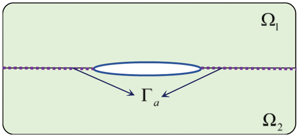
Figure 1: Sketches of isotropic body with a central crack

The geometric description of each discontinuous quadratic element is given as

xi=∑j=13Nj(ξ)xij,i=1,2,(6)

where xi(i=1,2) are coordinates of the point on the boundary element, xij(i=1,2;j=1,2,3) are coordinates of the left point, the middle point, and the right point of the element, ξ is the dimensionless coordinate with −1≤ξ≤1, and Nj(ξ)(j=1,2,3) are shape functions as

N1(ξ)=12(ξ2−ξ),N2(ξ)=1−ξ2,N3(ξ)=12(ξ2+ξ).(7)

The quantities (displacement and traction) on the boundary element are approximated by

w=∑j=13Njα(ξ)wj,andτ=∑j=13Njα(ξ)τj,(8)

where wj(j=1,2,3) and τj(j=1,2,3) are the values of displacement and traction at ξ=−α,0,α(0<α<1), respectively, and Njα(ξ)(j=1,2,3) are displacement/traction shape functions as

N1α(ξ)=12(ξ2α2−ξα),N2α(ξ)=1−ξ2α2,N3α(ξ)=12(ξ2α2+ξα).(9)

It should be noted that the parameter α in Eq. (8) is free to choose value from the region (0,1), which has little influence on the numerical accuracy of the present method.

Through the discretization of the BIE for sub-domains Ω1 and Ω2, we can form two linear equation systems as

(H1H1a)(w1w1a)=(G1G1a)(τ1τ1a),(10)

(H2H2a)(w2w2a)=(G2G2a)(τ2τ2a),(11)

where G and H denote the coefficient matrix, w is the vector of displacement, τ is the vector of traction, subscripts “1” and “2” of the physical quantities (displacement and traction) or coefficient matrix are used to distinguish sub-domains Ω1 and Ω2, and their superscript “a” is related with the auxiliary boundary Γa in Fig. 1. Based on the relationships of w1a=w2a and τ1a=−τ2a on Γa, Eqs. (10) and (11) have the coupling form as

(H1H1a00H2aH2)(w1waw2)=(G1G1a00−G2aG2)(τ1τaτ2),(12)

where wa=w1a(=w2a), and τa=τ1a(=τ2a). We can obtain the displacement and the traction on the boundary once Eq. (12) is solved.

Finally, the stress intensity factor (SIF) for mode III crack problems in thin-walled structures can be calculated as

KIII=μ42πrΔw(13)

where r denotes the distance between the crack tip and the near node on the crack surface, and Δw represents crack-opening-displacement (COD) at this near node. Obviously, Δw can be determined by using the value of the displacement on the crack surface which has been calculated by Eq. (12). The displacement extrapolation method is another way to calculate the SIF, which makes a linear extrapolation as

KIII=1α[KIII1−(1−α)KIII2](14)

where KIII1 and KIII2 are evaluated respectively by Eq. (13) at node ξ=−α and ξ=0 of the crack-tip element (crack-tip is at ξ=−1).

3.2 Special Crack-Tip Elements for the Displacement and the Stress

It is necessary to adopt special crack-tip elements for accurately simulating r-behavior in the near-tip displacement field and 1/r-behavior in the near-tip stress field. To satisfy this requirement, the displacement w in crack-tip element can be approximated as

w=∑j=13Mjα(ξ)wj=a1+a2r+a3r(15)

where Mjα(ξ)(j=1,2,3) are the special shape functions of displacements. Based on the location of the crack-tip, Mjα(ξ)(j=1,2,3) have two kinds of forms as

I)Crack-tip located at ξ=−1:Mjα(ξ)=Aj1α+Aj2α1+ξ+Aj3α(1+ξ),j=1,2,3(16)

II)Crack-tip located at ξ=1:Mjα(ξ)=Bj1α+Bj2α1−ξ+Bj3α(1−ξ),j=1,2,3(17)

where Ajiα(i=1,2,3) and Bjiα(i=1,2,3) can be determined by establishing a linear equation system as

Mjα(ξ)={1,ξatthe collocation node,0,ξat the other nodes.(18)

Finally, the displacement shape functions Mjα(ξ)(j=1,2,3) for the crack-tip elements with the crack-tip located at ξ=±1 have the formulations as

M1α(ξ)=α(1∓ξ−1)+ξ(1−1∓α)α(1+α−1)+α(1−α−1),(19)

M2α(ξ)=α(1+α∓1−α)−2α1∓ξ+ξ(1∓α−1±α)α(1+α−1)+α(1−α−1),(20)

M3α(ξ)=α(1∓ξ−1)+ξ(1±α−1)α(1+α−1)+α(1−α−1).(21)

On the other hand, the stress/traction in crack-tip element is approximated as

σ=∑j=13M^jα(ξ)σj=a^1+a^21r+a^3r(22)

where M^jα(ξ)(j=1,2,3) are the special shape functions of stresses/tractions. M^jα(ξ)(j=1,2,3) also have two different types of formulas which are given as

I)Crack-tip located at ξ=−1:M^jα(ξ)=A^j1α+A^j2α11+ξ+A^j3α1+ξ,j=1,2,3(23)

II)Crack-tip located at ξ=1:M^jα(ξ)=B^j1α+B^j2α11−ξ+B^j3α1−ξ,j=1,2,3(24)

where A^jiα(i=1,2,3) and B^jiα(i=1,2,3) can be obtained by

M^jα(ξ)={1,ξatthe collocation node,0,ξat the other nodes.(25)

The stress/traction shape functions M^jα(ξ)(j=1,2,3) for the crack-tip elements with the crack-tip located at ξ=±1 can be finally expressed as

M^1α(ξ)=1±α1∓ξ(1∓α+1)(1∓ξ−1)±ξ(1+α∓1)(1−α±1)∓α,(26)

M^2α(ξ)=11∓ξ(1+α−1∓ξ)(1−α−1∓ξ)(1+α−1)(1−α−1),(27)

M^3α(ξ)=1∓α1∓ξξ±(1±α+1)(1∓ξ−1)α±(1±α+1)(1∓α−1).(28)

3.3 Nearly Singular and Singular Integrals in the BEM Formulation

After the above-mentioned boundary element discretization, we have to deal with two types of nearly singular integrals [42] as

S1=∫−11ϕ1(ξ)ln⁡r2(ξ)dξ,andS2=∫−11ϕ2(ξ)1r2β(ξ)dξ,β>0(29)

where ϕi(ξ)(i=1,2) are regularized functions resulting from shape functions and Jacobian determinant of coordinate transformation, and r(ξ) is a distance between field point and source point expressed as [52]

r(ξ)=(ξ−η)2φ(ξ)+d2(30)

in which φ(ξ) is the positive function, η∈[−1,1] is the dimensionless projection coordinate of the field point near the boundary element, and d is the minimum distance between this field point to the near-boundary element. Replacing r(ξ) in Eq. (29) by its expression, we have

S1=∫−11ϕ1(ξ)ln⁡[(ξ−η)2φ(ξ)+d2]dξ,andS2=∫−11ϕ2(ξ)1[(ξ−η)2φ(ξ)+d2]βdξ(31)

Obviously, the above-mentioned integrals have near singularities when d is a small number.

The exponential transformation in [42,53] is applied to the regularization of nearly singular integrals. Firstly, we split Si(i=1,2) in Eq. (30) into two parts as

S1=[∫−1η+∫η1]ϕ1(ξ)ln⁡[(ξ−η)2φ(ξ)+d2]dξ,andS2=[∫−1η+∫η1]ϕ2(ξ)1[(ξ−η)2φ(ξ)+d2]βdξ(32)

and they can be recast as

S1=∫0η^ϕ1(ξ)ln⁡[(ξ−η)2φ(ξ)+d2]dξ,andS2=∫0η^ϕ2(ξ)1[(ξ−η)2φ(ξ)+d2]βdξ(33)

where η^ is a constant related with η. Next, we apply the exponential transformation ξ=d(eℓ(1+ζ)−1) with ℓ=ln⁡(1+η^/d)/2, which maps ξ(0,η^) to ζ(−1,1). Substituting this transformation into Eq. (32), one can obtain

S1=ℓd∫−11ϕ1(t){ln⁡[(eℓ(1+ζ)−1)2φ(t)+1]+ln⁡d2}eℓ(1+ζ)dζ,andS2=ℓd2β−1∫−11ϕ2(t)eℓ(1+ζ)[(eℓ(1+ζ)−1)2φ(t)+1]βdζ(34)

It is obvious that the above-mentioned integral has no near singularity when d is close to zero.

Singular integrals [54,55] also appeared in the boundary element discretization of the BIEs. In this work, a generally direct method [56] is applied for the regularization of these singular integrals. The details are not provided here, and the interested readers are referred to [56]. In addition, the Gaussian quadrature formula is used for all numerical integrations in this work.

4  Numerical Experiments

Three numerical experiments are provided to test the performance of the developed method. The numerical accuracy of the SIF calculated by the present approach is estimated by the relative error formulation [57,58] as

Relativeerror=|KIIINumerical−KIIIExactKIIIExact|.(35)

The displacement extrapolation method is used for calculating the SIF in all numerical examples, and α for all boundary elements is set to 0.5.

4.1 Test Problem 1: A Thin-Walled Structure with a Central Crack

As the first example, a thin-walled structure with a central crack is considered. The sketch of the structure is shown in Fig. 2. The length of the half crack is a. The thickness-to-length (TOL) ratio of the thin-walled structure is defined by b/H. The anti-plane shear loading τ0=1 is imposed on the upper and lower boundaries in Fig. 2. Traction-free condition is applied on the remaining boundaries and the crack surface. The analytical solution of the SIF (mode III) is given as

KIII=τ0πa2bπatan⁡(πa2b).(36)

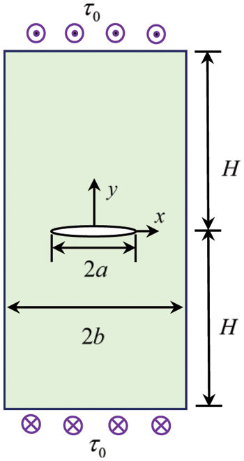
Figure 2: The sketch of a thin elastic body with a central crack

In the numerical simulation, H is set to be 10, and a/b=1/4. 40 discontinuous quadratic elements are adopted for the BIE discretization, and 4 of these elements are used on the crack surface. For the thin-walled structure with TOL ratio from 1E − 01 to 1E − 07, Fig. 3 plots the numerical error variation of the SIF by using the present method. As we can observe, the satisfied results are obtained by the developed approach with a small number of boundary elements even for the structure with TOL ratio of 1E − 07.

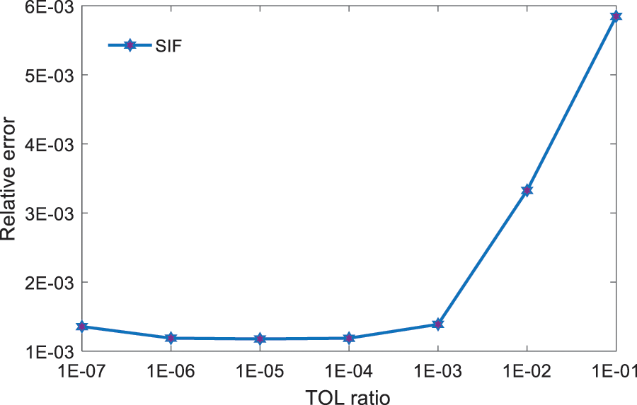
Figure 3: Relative errors of the SIF for the thin-walled structure with different TOL ratio

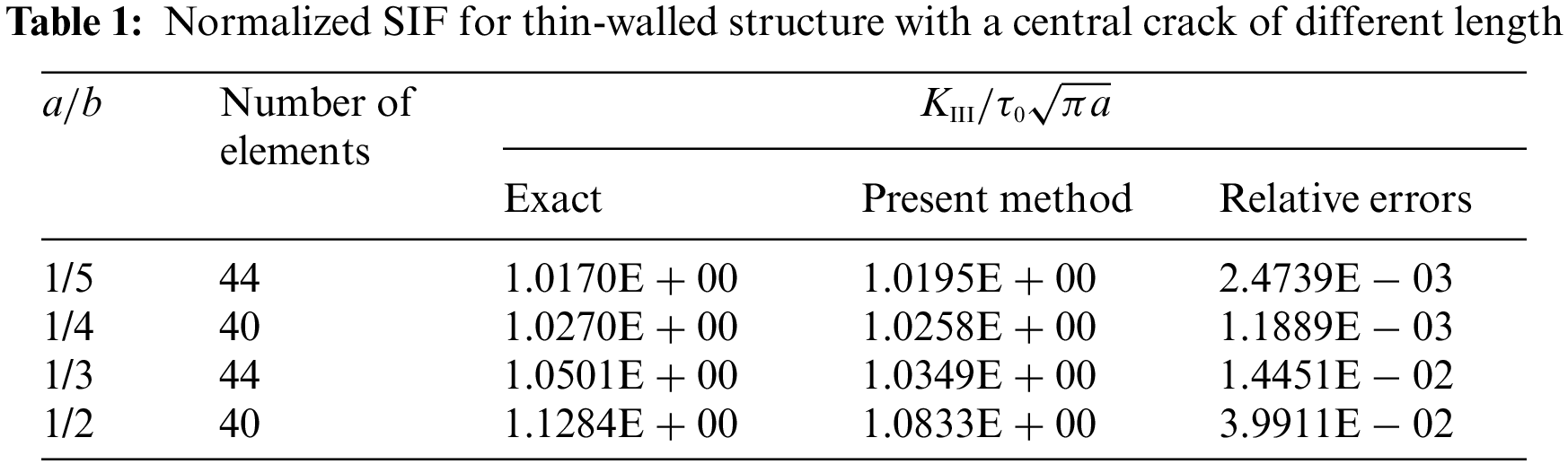
Next, the performance of the present method for solving the thin-walled structure with a central crack of different length is investigated. TOL ratio is set to IE − 06. Table 1 lists the numerical results of the normalized SIF. It can be found from this table that the numerical results have a good agreement with the exact solutions.

4.2 Test Problem 2: A Thin-Walled Structure with an Edge Crack

As the second example, we consider a thin-walled structure with an edge crack, and Fig. 4 shows its dimension. The crack length is a, and the TOL ratio of this structure is also defined by b/H. The anti-plane shear loading τ0=1 is imposed on the upper and lower boundaries. Traction-free condition is used on the crack surface and the remaining boundaries. Exact solution of the SIF (mode III) is same as that of the example 1. In this example, H is set to be 10, and b=3a.

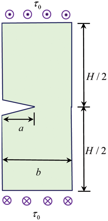
Figure 4: The sketch of a thin elastic body with an edge crack

We use 36 discontinuous quadratic elements including 4 elements on the crack surface in the numerical simulation of the present method and the conventional BEM. Here, nearly singular integrals are directly calculated by standard Gaussian quadrature in the conventional BEM. Table 2 gives the numerical results of normalized SIF KIII/(τ0πa) for the TOL ratio from 1E − 01 to 1E − 08.

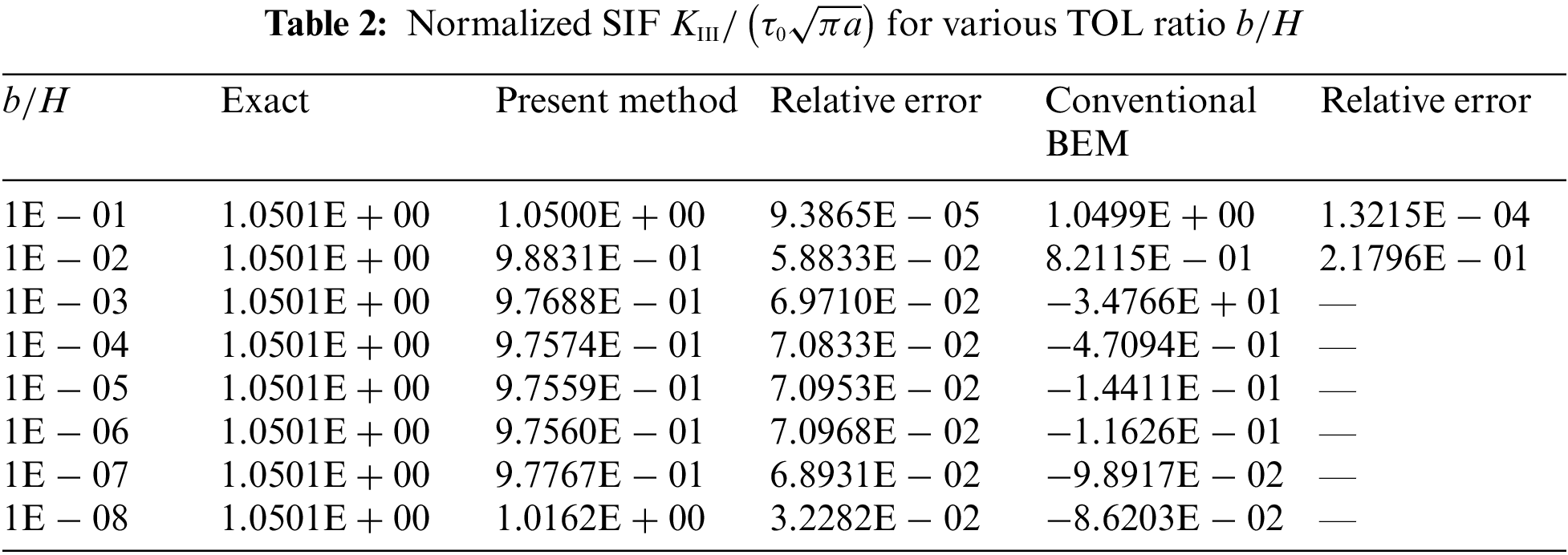
Obviously, the present method yields accurate results even for the TOL of 1E − 08, but the conventional BEM is invalid when the TOL is less than 1E − 02.

4.3 Test Problem 3: A Thin-Walled Structure with a Semi-Infinite Crack

A thin-walled structure with a semi-infinite crack (see Fig. 5) is investigated as the third example, in which the TOL ratio of the structure is defined by h/L. As shown in Fig. 5, the upper and lower boundaries are subject to the displacement constraint w=0, and the crack surface imposes the anti-plane shear loading τ0=1. Traction-free condition is used on the left and right boundaries. Exact solution of the SIF (mode III) is expressed as

KIII=τ02h.(37)

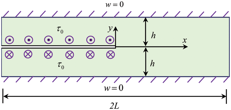
Figure 5: The sketch of a thin elastic body with a semi-infinite crack

L is set to 10 in this case.

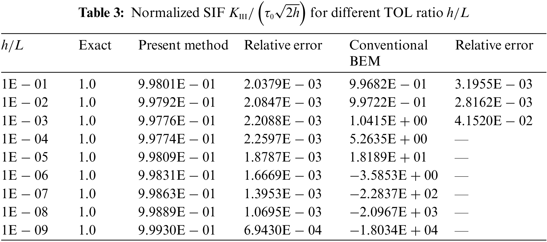
In this simulation, 180 discontinuous quadratic elements including 34 elements on the crack surface are used for the present method and the conventional BEM. For the thin-walled structure with the TOL ratio from 1E − 01 to 1E − 09, the numerical results of normalized SIF KIII/(τ02h) calculated by above-mentioned two approaches are shown in Table 3. As we can see from this table, the present method has a good performance for different TOL ratio, especially for TOL ratio of 1E − 09. However, the conventional BEM can obtain accurate results only when the TOL ration is not great than 1E − 03.

5  Conclusion and Generalization

A novel numerical framework for mode III crack problems of thin-walled structures is presented by combining several advanced techniques in the BEM literature. The displacement and stress shape functions of special crack-tip elements are derived in detail. Moreover, an exponential transformation technique is applied for the nearly singular integrals resulting from these special structures. Mode III crack problems for thin-walled structures with a central, edge or semi-infinite crack are investigated by the developed method. Numerical results illustrate that the present approach obtains accurate numerical results for ultra-thin structures even with the TOL ration of 1E − 09. The present scheme can be extended for 3D crack problems of thin-walled structures, which will be reported in the near future.

Funding Statement: The research was supported by the National Natural Science Foundation of China (No. 11802165), and the China Postdoctoral Science Foundation (Grant No. 2019M650158).

Conflicts of Interest: The authors declare that they have no conflicts of interest to report regarding the present study.

References

1. Zerbst, U., Heinimann, M., Dalle Donne, C., Steglich, D. (2009). Fracture and damage mechanics modelling of thin-walled structures–An overview. Engineering Fracture Mechanics, 76(1), 5–43. [Google Scholar]
2. Guarracino, F., Walker, A. (2008). Some comments on the numerical analysis of plates and thin-walled structures. Thin-Walled Structures, 46(7–9), 975–980. [Google Scholar]
3. Xu, S., Li, W., Li, L., Li, T., Ma, C. (2022). Crashworthiness design and multi-objective optimization for bio-inspired hierarchical thin-walled structures. Computer Modeling in Engineering & Sciences, 131(2), 929–947. https://doi.org/10.32604/cmes.2022.018964 [Google Scholar] [CrossRef]
4. Dong, H. W., Zhao, S. D., Wang, Y. S., Zhang, C. (2017). Topology optimization of anisotropic broadband double-negative elastic metamaterials. Journal of the Mechanics and Physics of Solids, 105, 54–80. [Google Scholar]
5. Zhao, S. D., Chen, A. L., Wang, Y. S., Zhang, C. (2018). Continuously tunable acoustic metasurface for transmitted wavefront modulation. Physical Review Applied, 10(5), 054066. [Google Scholar]
6. Qu, W., He, H. (2022). A GFDM with supplementary nodes for thin elastic plate bending analysis under dynamic loading. Applied Mathematics Letters, 124, 107664. [Google Scholar]
7. Sukumar, N., Moës, N., Moran, B., Belytschko, T. (2000). Extended finite element method for three-dimensional crack modelling. International Journal for Numerical Methods in Engineering, 48(11), 1549–1570. [Google Scholar]
8. Surendran, M., Natarajan, S., Palani, G., Bordas, S. P. (2019). Linear smoothed extended finite element method for fatigue crack growth simulations. Engineering Fracture Mechanics, 206, 551–564. [Google Scholar]
9. Chai, Y., Li, W., Liu, Z. (2022). Analysis of transient wave propagation dynamics using the enriched finite element method with interpolation cover functions. Applied Mathematics and Computation, 412, 126564. [Google Scholar]
10. Wang, J., Jiang, W., Wang, Q. (2019). Numerical simulation and experimental studies on elastic-plastic fatigue crack growth. Computer Modeling in Engineering & Sciences, 118(2), 377–395. https://doi.org/10.31614/cmes.2019.01836 [Google Scholar] [CrossRef]
11. Li, W., Zhang, Q., Gui, Q., Chai, Y. (2021). A coupled FE-meshfree triangular element for acoustic radiation problems. International Journal of Computational Methods, 18(3), 2041002. [Google Scholar]
12. Li, H., Li, J., Yuan, H. (2018). A review of the extended finite element method on macrocrack and microcrack growth simulations. Theoretical and Applied Fracture Mechanics, 97, 236–249. [Google Scholar]
13. Gu, Y., Zhang, C. (2020). Novel special crack-tip elements for interface crack analysis by an efficient boundary element method. Engineering Fracture Mechanics, 239, 107302. [Google Scholar]
14. He, S., Wang, C., Zhou, X., Dong, L., Atluri, S. N. (2022). Weakly singular symmetric galerkin boundary element method for fracture analysis of three-dimensional structures considering rotational inertia and gravitational forces. Computer Modeling in Engineering & Sciences, 131(3), 1857–1882. https://doi.org/10.32604/cmes.2022.019160 [Google Scholar] [CrossRef]
15. Lei, J., Zhang, C. (2018). A simplified evaluation of the mechanical energy release rate of kinked cracks in piezoelectric materials using the boundary element method. Engineering Fracture Mechanics, 188, 36–57. [Google Scholar]
16. Xie, G., Zhou, F., Li, H., Wen, X., Meng, F. (2019). A family of non-conforming crack front elements of quadrilateral and triangular types for 3D crack problems using the boundary element method. Frontiers of Mechanical Engineering, 14(3), 332–341. [Google Scholar]
17. Liu, Y., Li, Y., Xie, W. (2017). Modeling of multiple crack propagation in 2-D elastic solids by the fast multipole boundary element method. Engineering Fracture Mechanics, 172, 1–16. [Google Scholar]
18. Gu, Y., Zhang, C. (2021). Fracture analysis of ultra-thin coating/substrate structures with interface cracks. International Journal of Solids and Structures, 225, 111074. [Google Scholar]
19. Gu, Y., Lin, J., Wang, F. (2021). Fracture mechanics analysis of bimaterial interface cracks using an enriched method of fundamental solutions: Theory and MATLAB code. Theoretical and Applied Fracture Mechanics, 116, 103078. [Google Scholar]
20. Xia, H., Gu, Y. (2021). Generalized finite difference method for electroelastic analysis of three-dimensional piezoelectric structures. Applied Mathematics Letters, 117, 107084. [Google Scholar]
21. Jiang, S., Gu, Y., Fan, C. M., Qu, W. (2021). Fracture mechanics analysis of bimaterial interface cracks using the generalized finite difference method. Theoretical and Applied Fracture Mechanics, 113, 102942. https://doi.org/10.1016/j.tafmec.2021.102942 [Google Scholar] [CrossRef]
22. Qu, W., He, H. (2020). A spatial–temporal GFDM with an additional condition for transient heat conduction analysis of FGMs. Applied Mathematics Letters, 110, 106579. https://doi.org/10.1016/j.aml.2020.106579 [Google Scholar] [CrossRef]
23. Li, J., Zhang, L., Qin, Q. H. (2021). A regularized method of moments for three-dimensional time-harmonic electromagnetic scattering. Applied Mathematics Letters, 112, 106746. https://doi.org/10.1016/j.aml.2020.106746 [Google Scholar] [CrossRef]
24. Li, P. W. (2021). Space–time generalized finite difference nonlinear model for solving unsteady Burgers’ equations. Applied Mathematics Letters, 114, 106896. https://doi.org/10.1016/j.aml.2020.106896 [Google Scholar] [CrossRef]
25. Qiu, L., Zhang, M., Qin, Q. H. (2021). Homogenization function method for time-fractional inverse heat conduction problem in 3D functionally graded materials. Applied Mathematics Letters, 122, 107478. https://doi.org/10.1016/j.aml.2021.107478 [Google Scholar] [CrossRef]
26. Wang, F., Wang, C., Chen, Z. (2020). Local knot method for 2D and 3D convection–diffusion–reaction equations in arbitrary domains. Applied Mathematics Letters, 105, 106308. https://doi.org/10.1016/j.aml.2020.106308 [Google Scholar] [CrossRef]
27. Wang, F., Fan, C. M., Zhang, C., Lin, J. (2020). A localized space-time method of fundamental solutions for diffusion and convection-diffusion problems. Advances in Applied Mathematics and Mechanics, 12(4), 940–958. https://doi.org/10.4208/aamm.OA-2019-0269 [Google Scholar] [CrossRef]
28. Fu, Z., Tang, Z., Xi, Q., Liu, Q., Gu, Y. et al. (2022). Localized collocation schemes and their applications. Acta Mechanica Sinica, 38(7), 1–28. https://doi.org/10.1007/s10409-022-22167-x [Google Scholar] [CrossRef]
29. Fu, Z. J., Xie, Z. Y., Ji, S. Y., Tsai, C. C., Li, A. L. (2020). Meshless generalized finite difference method for water wave interactions with multiple-bottom-seated-cylinder-array structures. Ocean Engineering, 195, 106736. https://doi.org/10.1016/j.oceaneng.2019.106736 [Google Scholar] [CrossRef]
30. Tang, Z., Fu, Z., Chen, M., Huang, J. (2022). An efficient collocation method for long-time simulation of heat and mass transport on evolving surfaces. Journal of Computational Physics, 111310. https://doi.org/10.1016/j.jcp.2022.111310 [Google Scholar] [CrossRef]
31. Li, Y., Dang, S., Li, W., Chai, Y. (2022). Free and forced vibration analysis of two-dimensional linear elastic solids using the finite element methods enriched by interpolation cover functions. Mathematics, 10(3), 456. https://doi.org/10.3390/math10030456 [Google Scholar] [CrossRef]
32. Han, Y., Yan, Z., Lin, J., Feng, W. (2022). A novel model and solution on the bending problem of arbitrary shaped magnetoelectroelastic plates based on the modified strain gradient theory. Journal of Intelligent Material Systems and Structures, 33(8), 1072–1086. https://doi.org/10.1177/1045389X211041173 [Google Scholar] [CrossRef]
33. Feng, W., Yan, Z., Lin, J., Zhang, C. (2020). Bending analysis of magnetoelectroelastic nanoplates resting on pasternak elastic foundation based on nonlocal theory. Applied Mathematics and Mechanics, 41(12), 1769–1786. https://doi.org/10.1007/s10483-020-2679-7 [Google Scholar] [CrossRef]
34. Ju, B., Qu, W. Z. (2022). Three-dimensional application of the meshless generalized finite difference method for solving the extended Fisher-Kolmogorov equation. Applied Mathematics Letters. https://doi.org/10.1016/j.aml.2022.108458 [Google Scholar] [CrossRef]
35. Li, X., Li, S. (2021). A fast element-free galerkin method for the fractional diffusion-wave equation. Applied Mathematics Letters, 122, 107529. https://doi.org/10.1016/j.aml.2021.107529 [Google Scholar] [CrossRef]
36. Xie, G., Zhou, F., Zhang, J., Zheng, X., Huang, C. (2013). New variable transformations for evaluating nearly singular integrals in 3D boundary element method. Engineering Analysis with Boundary Elements, 37(9), 1169–1178. https://doi.org/10.1016/j.enganabound.2013.05.005 [Google Scholar] [CrossRef]
37. Zhang, Y., Gong, Y., Gao, X. (2015). Calculation of 2D nearly singular integrals over high-order geometry elements using the sinh transformation. Engineering Analysis with Boundary Elements, 60, 144–153. https://doi.org/10.1016/j.enganabound.2014.12.006 [Google Scholar] [CrossRef]
38. Gu, Y., Chen, W., Zhang, B., Qu, W. (2014). Two general algorithms for nearly singular integrals in two dimensional anisotropic boundary element method. Computational Mechanics, 53(6), 1223–1234. https://doi.org/10.1007/s00466-013-0965-1 [Google Scholar] [CrossRef]
39. Zhang, Y., Li, X., Sladek, V., Sladek, J., Gao, X. (2015). A new method for numerical evaluation of nearly singular integrals over high-order geometry elements in 3D BEM. Journal of Computational and Applied Mathematics, 277, 57–72. https://doi.org/10.1016/j.cam.2014.08.027 [Google Scholar] [CrossRef]
40. Niu, Z., Hu, Z., Cheng, C., Zhou, H. (2015). A novel semi-analytical algorithm of nearly singular integrals on higher order elements in two dimensional BEM. Engineering Analysis with Boundary Elements, 61, 42–51. https://doi.org/10.1016/j.enganabound.2015.06.007 [Google Scholar] [CrossRef]
41. Zhang, Y., Qu, W., Gu, Y. (2013). Evaluation of singular and nearly singular integrals in the BEM with exact geometrical representation. Journal of Computational Mathematics, 355–369. https://doi.org/10.4208/jcm [Google Scholar] [CrossRef]
42. Zhang, Y. M., Qu, W. Z., Chen, J. T. (2013). BEM analysis of thin structures for thermoelastic problems. Engineering Analysis with Boundary Elements, 37(2), 441–452. https://doi.org/10.1016/j.enganabound.2012.11.012 [Google Scholar] [CrossRef]
43. Wang, J., Qu, W., Wang, X., Xu, R. P. (2022). Stress analysis of elastic bi-materials by using the localized method of fundamental solutions. AIMS Mathematics, 7(1), 1257–1272. https://doi.org/10.3934/math.2022074 [Google Scholar] [CrossRef]
44. Gu, Y., Fan, C. M., Fu, Z. (2021). Localized method of fundamental solutions for three-dimensional elasticity problems: Theory. Advances in Applied Mathematics and Mechanics, 13(6), 1520–1534. https://doi.org/10.4208/aamm [Google Scholar] [CrossRef]
45. Chen, Z., Wang, F. (2021). On the supporting nodes in the localized method of fundamental solutions for 2D potential problems with Dirichlet boundary condition. AIMS Mathematics, 6(7), 7056–7069. https://doi.org/10.3934/math.2021414 [Google Scholar] [CrossRef]
46. Wang, F., Zhao, Q., Chen, Z., Fan, C. M. (2021). Localized chebyshev collocation method for solving elliptic partial differential equations in arbitrary 2D domains. Applied Mathematics and Computation, 397, 125903. https://doi.org/10.1016/j.amc.2020.125903 [Google Scholar] [CrossRef]
47. Xi, Q., Fu, Z., Wu, W., Wang, H., Wang, Y. (2021). A novel localized collocation solver based on Trefftz basis for potential-based inverse electromyography. Applied Mathematics and Computation, 390, 125604. https://doi.org/10.1016/j.amc.2020.125604 [Google Scholar] [CrossRef]
48. Aliabadi, M. H. (2002). Applications in solids and structures, vol. 2. New York: John Wiley & Sons. [Google Scholar]
49. Song, L., Li, P. W., Gu, Y., Fan, C. M. (2020). Generalized finite difference method for solving stationary 2D and 3D Stokes equations with a mixed boundary condition. Computers & Mathematics with Applications, 80(6), 1726–1743. https://doi.org/10.1016/j.camwa.2020.08.004 [Google Scholar] [CrossRef]
50. Tang, Z., Fu, Z., Chen, M., Ling, L. (2021). A localized extrinsic collocation method for turing pattern formations on surfaces. Applied Mathematics Letters, 122, 107534. https://doi.org/10.1016/j.aml.2021.107534 [Google Scholar] [CrossRef]
51. Xing, Y., Song, L., He, X., Qiu, C. (2020). A generalized finite difference method for solving elliptic interface problems. Mathematics and Computers in Simulation, 178, 109–124. https://doi.org/10.1016/j.matcom.2020.06.006 [Google Scholar] [CrossRef]
52. Zhang, Y. M., Gu, Y., Chen, J. T. (2011). Boundary element analysis of 2D thin walled structures with high-order geometry elements using transformation. Engineering Analysis with Boundary Elements, 35(3), 581–586. https://doi.org/10.1016/j.enganabound.2010.07.008 [Google Scholar] [CrossRef]
53. Zhang, Y., Gu, Y., Chen, J. T. (2010). Boundary element analysis of the thermal behaviour in thin-coated cutting tools. Engineering Analysis with Boundary Elements, 34(9), 775–784. https://doi.org/10.1016/j.enganabound.2010.03.014 [Google Scholar] [CrossRef]
54. Zheng, C., Matsumoto, T., Takahashi, T., Chen, H. (2011). Explicit evaluation of hypersingular boundary integral equations for acoustic sensitivity analysis based on direct differentiation method. Engineering Analysis with Boundary Elements, 35(11), 1225–1235. https://doi.org/10.1016/j.enganabound.2011.05.004 [Google Scholar] [CrossRef]
55. Zheng, C. J., Gao, H. F., Du, L., Chen, H. B., Zhang, C. (2016). An accurate and efficient acoustic eigensolver based on a fast multipole BEM and a contour integral method. Journal of Computational Physics, 305, 677–699. https://doi.org/10.1016/j.jcp.2015.10.048 [Google Scholar] [CrossRef]
56. Guiggiani, M., Casalini, P. (1987). Direct computation of Cauchy principal value integrals in advanced boundary elements. International Journal for Numerical Methods in Engineering, 24(9), 1711–1720. https://doi.org/10.1002/(ISSN)1097-0207 [Google Scholar] [CrossRef]
57. Qu, W., Gao, H., Gu, Y. (2021). Integrating Krylov deferred correction and generalized finite difference methods for dynamic simulations of wave propagation phenomena in long-time intervals. Advances in Applied Mathematics and Mechanics, 13(6), 1398–1417. https://doi.org/10.4208/aamm.OA-2020-0178 [Google Scholar] [CrossRef]
58. Wang, C., Wang, F., Gong, Y. (2021). Analysis of 2D heat conduction in nonlinear functionally graded materials using a local semi-analytical meshless method. AIMS Mathematics, 6(11), 12599–12618. https://doi.org/10.3934/math.2021726 [Google Scholar] [CrossRef]
Cite This Article
Copyright © 2023 The Author(s). Published by Tech Science Press.
This work is licensed under a Creative Commons Attribution 4.0 International License , which permits unrestricted use, distribution, and reproduction in any medium, provided the original work is properly cited.
Downloads
Citation Tools