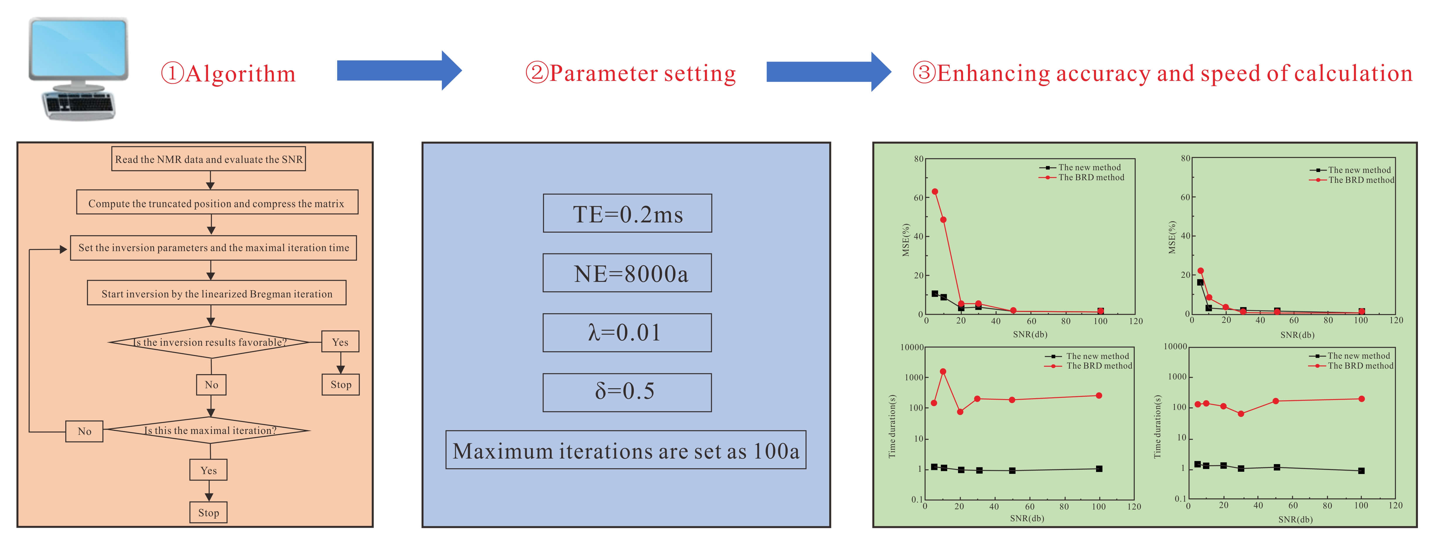
A Novel Method to Enhance the Inversion Speed and Precision of the NMR T₂ Spectrum by the TSVD Based Linearized Bregman Iteration

1  Introduction

The time domain signal determined by the low field nuclear magnetic resonance (NMR) can be used to detect many features of the porous rock, such as the pore size distribution, pore connectivity, wettability, viscosity, as well as fluid saturation [1–4]. The decaying signals are inverted to the time domain spectrums, which are frequently related to the formation evaluation and petrophysical study. However, the inversion of the NMR data is usually ill-posed, resulting in significant difficulty in the computation precision and efficiency. To deal with this problem, many attempts and developments have been tried in recent decades, which can be summarized into three categories: iterative algorithms, regularization algorithms and intelligent algorithms [5–7]. However, there are many drawbacks for these existing algorithms. Firstly, for the iterative algorithms, such as the truncated singular value decomposition (TSVD), the nonnegative least squares (NNLS) and the simultaneous iterative reconstruction technique (SIRT), the initial guess and the iteration criterion are hard to be determined [8–10]. Moreover, some unwanted signals are introduced during the iteration process, leading to the misinterpretation of the results [11]. Secondly, for the regularized algorithms, such as the Butler-Reeds-Dawson (BRD) algorithm and the maximum entropy algorithm, the penalty term and the regularization parameters are difficult to estimate [12,13]. In addition, it has the risk of trapping in local minimal values. Thirdly, although some intelligent algorithms, such as the simulated annealing and the differential evolution can reach favorable inversion result at certain conditions, they are immature and not used massively. In recent years, some researchers utilized the L1 regularization to invert the raw decaying data to spectrums and achieved favorable results [14–17].

The Bregman iteration is considered as an effective method for solving constrained optimization problems. It has been widely applied in many fields such as seismic prospecting, image reconstruction, as well as noise reduction [18–21]. The best advantage of the Bregman iteration is the easy convergence [20]. Therefore, it is introduced into the NMR inversion, aiming to get the stable solution at a favorable iteration time. In this paper, the novel method composed by the combination of improved TSVD and the linearized Bregman iteration is investigated. And then, it is validated by comparing its results with those of other previous algorithms.

2  NMR Relaxation Theory

Based on the basic principle NMR theory, the longitudinal relaxation time (T1) and the transversal relaxation time (T2) are used to depict the polarizing and decaying behaviors during the nuclear precession process, which are given by [1,2]:

1T1=1T1b+1T1s=1T1b+ρ1sSV(1)

1T2=1T2b+1T2s+1T2d=1T2b+ρ2sSV+1T2d(2)

where T1b and T2b are the bulk relaxation times of T1 and T2, determined by the intrinsic properties of the fluids such as viscosity and chemical compositions; T1s and T2s are the surface relaxation times of T1 and T2, controlled by the properties of fluid-rock interface such as pore size and surface relaxivity; T2d is the diffusional relaxation time of T2, affected by the diffusion coefficient, temperature and pressure; S/V is the pore surface to volume ratio; ρ1s and ρ2s are the surface relaxivities of T1 and T2, respectively [2].

T2 is the most frequently measured parameter in conventional low-field NMR experiments and logging, which are obtained by Carr-Purcell-Meiboom-Gill (CPMG) pulse sequence. Therefore, only the inversion problem of T2 is examined in this study. The discrete relationship between the magnetization intensity and T2 satisfies the following equation:

f(t)=f0∑i=1naiexp⁡(−t/T2i)+ε(t).(3)

where ai is the volume fraction of the i-th relaxation component decaying with relaxation time of T2; f0 is the initial magnetization intensity; t is the evolution time; n is the number of T2, which is always predefined as the exponent of 2, such as 32, 64, and 128; ε(t) is the recorded noise.

In the conventional inversion algorithms, Eq. (3) is expressed as the optimization form with nonnegative constraints.

min||F−AX||2s.t.x(j)≥0forj=1,2,…,n(4)

where F is recorded magnetic intensity with the size of m×1, A is the kernel matrix with the size of m×n, and X is the T2 with the size of n×1.

Since A is ill-conditioned, the optimization problem is an ill-posed problem. The solution with the minimal fitting residual is easily contaminated by noise.

3  Methodology

It is often the case that most elements in the spectrum are zeros, so L1 penalty term is added into the function to enforce the sparsity of the spectrum. Therefore, the cost function is expressed as [18–21]:

minx(j)≥012||F−AX||22+λ||X||1(5)

where ||X||1 denotes the one-norm of X; λ is the regularization factor, which provides a tradeoff between fidelity-to-data and the noise sensitivity.

3.1 The Linearized Bregman Iteration

The Bregman iteration is very popular in many optimization problems due to its very nice convergence properties, including monotonic decrease in the residual term, convergence to the original signal, and convergence in terms of Bregman distance to the original signal with noisy data [22].

Assuming J(x) is a differentiable convex function (Bregman function), the Bregman distance between two points is given by [18–22]:

DJ(x,y)=J(x)−J(y)−<p,x−y>.(6)

where p∈∂J(x) is the subgradient of J(x).

The Bregman distance has several nice properties that make it an efficient tool for solving L1 regularization problems. Using the Bregman function, the optimization problem is transformed as:

minx(j)≥0{J(x)+H(x,f)}(7)

where J(x)=λ||X||1 and H(x,f)=12||F−AX||22.

Consequently, the key steps of the Bregman iteration are expressed as follows:

xk+1=argmin{DJpk(x,xk)+H(x,f)}(8)

pk+1=pk−∇H(xk+1,f)∈∂J(xk+1)(9)

where k denotes the iteration time.

The main function of Eq. (8) is to update the iterative solution, and the main function of Eq. (9) is to update the search direction for a new iteration. Due to the complexity of the computation of the subgradient, the simplified iteration operators are given by [23]:

fk+1=f−(Axk−fk)(10)

xk+1=minJ(x)+12||Ax−fk+1||22(11)

Then the problem is transformed to find the optimal values to satisfy Eqs. (8) or (11), which can be computationally expensive. Here we adopt the linearized version of the Bregman iteration to accelerate the computation since the minimization of Eq. (8) can be replaced by a minimization step that can be solved exactly.

The first order Taylor expansion of H(x,f) is expressed as:

H(x,f)=H(xk,f)+<∇H(xk,f),xk−x>(12)

By adding the penalty term of 12δ||x−xk||22 , the iteration in Eq. (8) is then transformed as:

xk+1=argminDJpk(x,xk)+H(xk,f)+<∇H(xk,f),xk−x>+12δ||x−xk||22(13)

Substituting Eq. (4) into Eq. (13), the iteration form is derived as:

xk+1=argminDJpk(x,xk)+12δ||x−(xk−1δAT(Axk−f))||22(14)

Eq. (9) is equivalent to:

pk+1=pk−δ(xk+1−(xk−1δAT(Axk−f)))(15)

Combining vk+1=∑j=0kAT(f−Axj) and Eq. (14) gives:

xik+1={1δ(vik−λ)vik∈(λ,+∞)0vik∈[−λ,λ]1δ(vik+λ)vik∈(−∞,−λ)(16)

Hence, the implementation of the linearized Bregman algorithm is as follows: (1) Initialize the values of x and v, iteration time of k and the maximal iteration time T, and the deviation of the stop criterion ξ; (2) Do the iterations of Eqs. (15) and (16) when ||Axk−f||>ξ or k<T; (3) Break the iteration by the stop criterion, and output the solution.

3.2 The Empirical TSVD

The above section gives the full part of the linearized Bregman iteration. However, direct application of this algorithm is impossible since the ill-conditioned kernel matrix A. So some pretreatments are necessary to ensure suitability. SVD is the effective method to decompose the ill-conditioned matrix, which is expressed as [23–25]:

A=USVT(17)

where U=[u1,u2,…,um] and V=[v1,v2,…,vn] are orthogonal matrices with the size of m×m and n×n; S=diag(s1,s2,…,sr) is the diagonal matrix with the size of m×n, and r=min(m,n).

Singular values of S are ordered as:

s1≥s2≥⋅⋅⋅≥sr=0(18)

It should be noted that singular values decay quickly to zero, and small singular values are often considered harmful components since they will result in the large error of the solutions. Conventional methods are to set a threshold and drop values smaller than the threshold such as the generalized cross validation (GCV), L curve, and signal to noise ratio (SNR) based methods [26].

Through many times of simulations trials, an empirical equation is established to predict the proper truncated position and can be expressed by:

q=a×SNRb(19)

where a and b are fitting parameters. In this study, they are 2.869 and 0.438, respectively.

Therefore, the kernel matrix is expressed as [27,28]:

Aq=UqSqVqT(20)

where Uq=(u1,u2,…,uq), Sq=(s1,s2,…,sq) and Vq=(v1,v1,…,vq).

Therefore, the iteration function for Eq. (15) is expressed as:

pk+1=pk−δ(xk+1−(xk−1δ(xk−VqSq−1UqTf))(21)

The space complexity, time complexity, and computational complexity for Aq are 3q2, 4q3, and O(q3), respectively. Hence, the computational complexity is greatly decreased by O(m2n)/O(q3) since q is much smaller than m and n. The flowchart of the proposed inversion method is shown in Fig. 1.

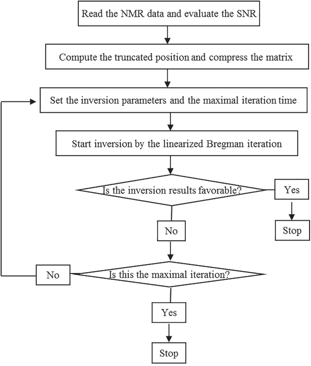
Figure 1: The flowchart of the proposed inversion algorithm

4  Numerical Examples

The simulation tests are conducted to verify the proposed novel inversion method using two typical distributions of the T2 spectrum, including the unimodal spectrum, the bimodal spectrum. Moreover, numerical data with different SNRs will be used to investigate the noise tolerance of this method. In our simulation, the noise is added using the in-built ‘awgn’ function of the Matlab software. It is typical additive Gaussian white noise. The SNR is specified with dB. All the simulations are conducted on a computer labeled the ‘OptiPlex 7050’ with the Intel(R) Core(TM) i7-7700 CPU @ 3.60 GHz. In the simulation, the echo spacing (TE) and the number of echoes are set as 0.2 ms and 8000, respectively. After many runs of simulations, λ and δ are found to be 0.01 and 0.5, respectively. The maximal iterations are set as 100. The total duration for each inversion is only about 1.2 s, which is suitable for both laboratory investigations and field applications. For comparison, the conventionally used method named ‘BRD’ is also used.

4.1 The Unimodal Spectrum

The Gaussian’s function is used to establish the forward unimodal distributed T2 spectrum with a peak of 10 ms and the decaying signals with SNR of 100, 50, 30, 20, 10, and 5, respectively. It should be noted that for simplicity, the normalized amplitude less than 0.003 is dropped and the spectrum is then renormalized. The simulated echo trains are shown in Fig. 2. The inverted spectrums are presented in Fig. 3. It can be seen that for the echo with SNR higher than 20, the inverted spectrum is strongly consistent with the forward model. However, if the SNR is lower than 10, the inverted results deviate from the model, but the peak position is only slightly moved. The inversion inaccuracy can be attributed to the contamination of the noise. However, the inversion results obtained by the BRD method deviate from the true value obviously at the SNR lower than 20.

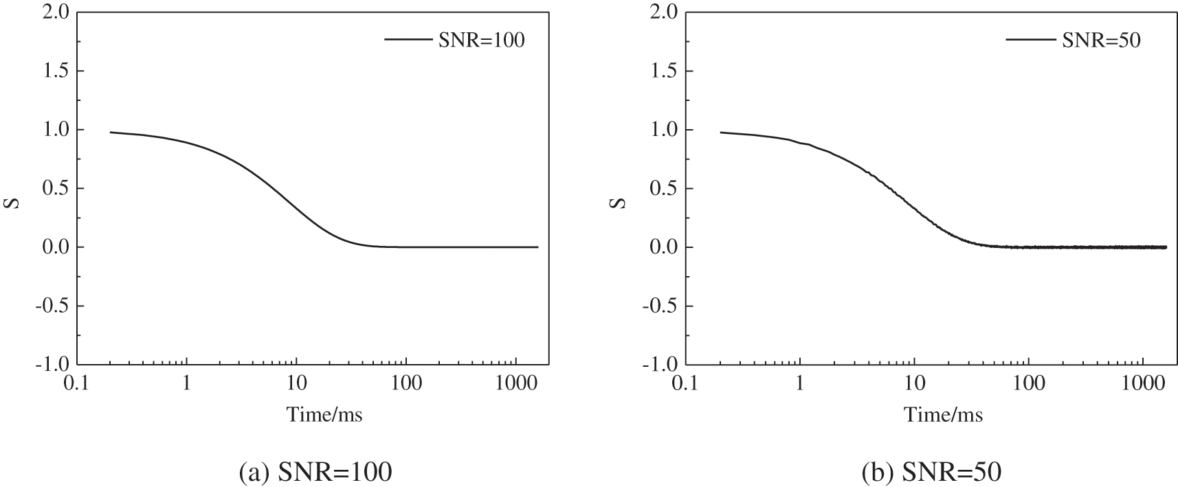
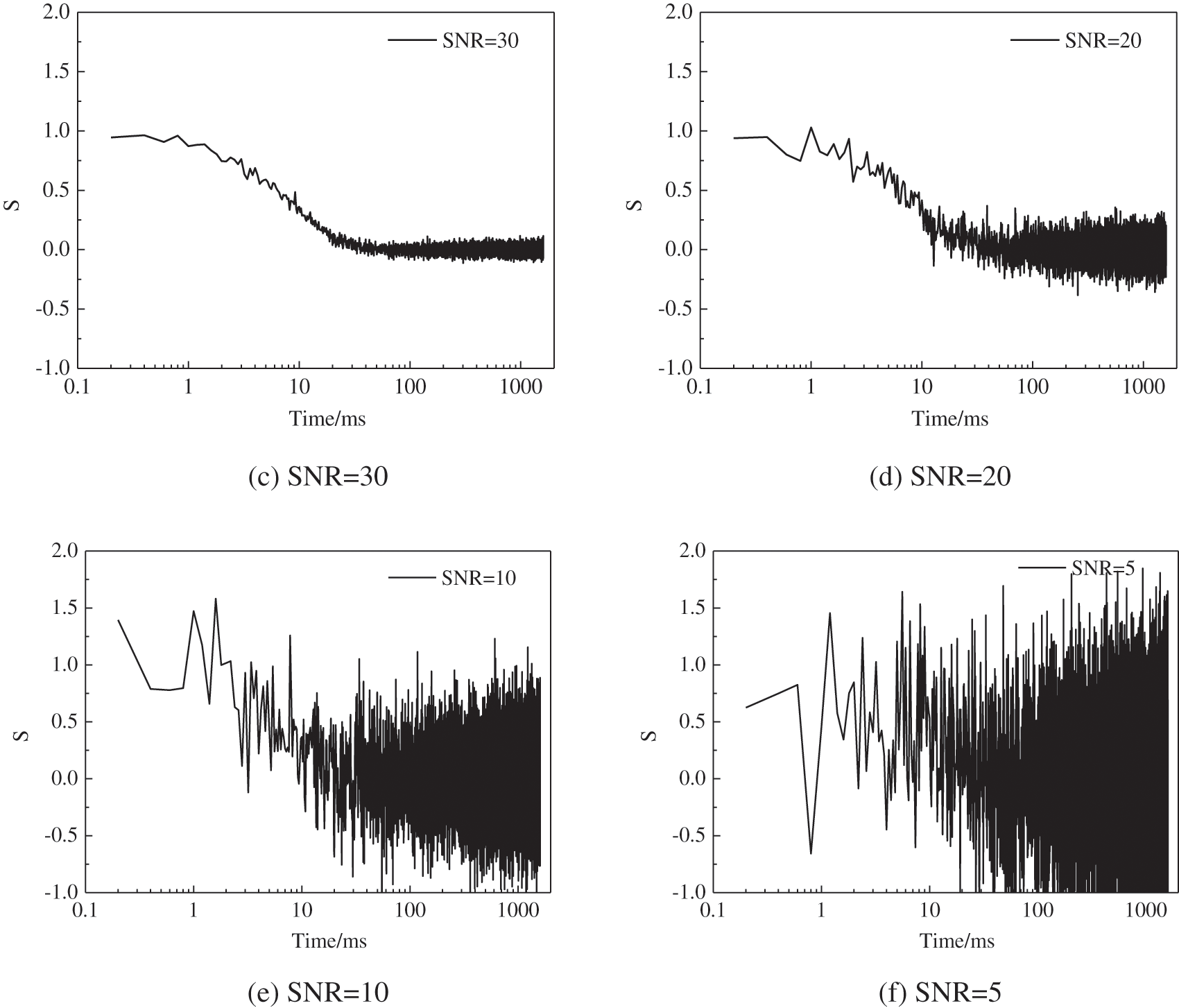
Figure 2: Simulated NMR trains of the unimodal spectrum with different SNRs

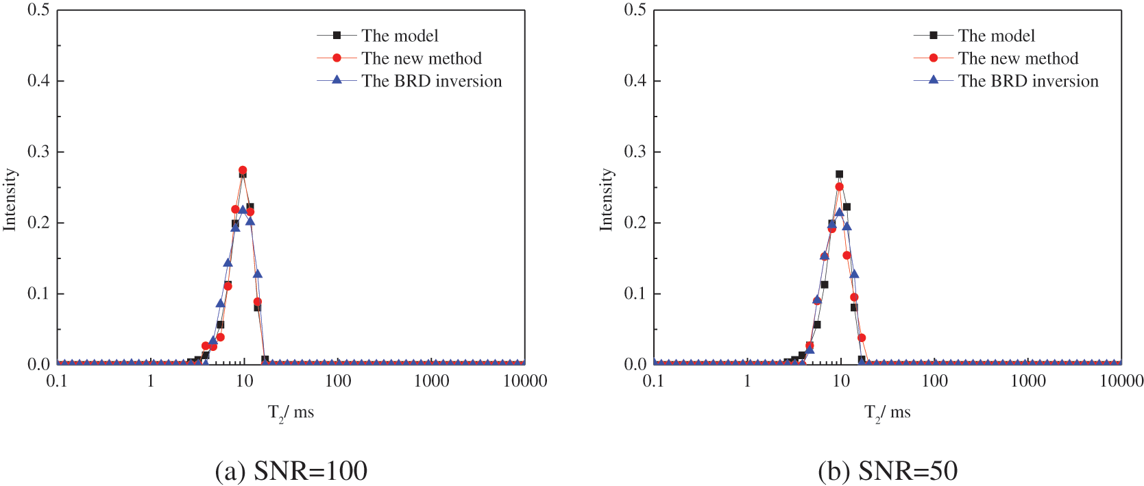
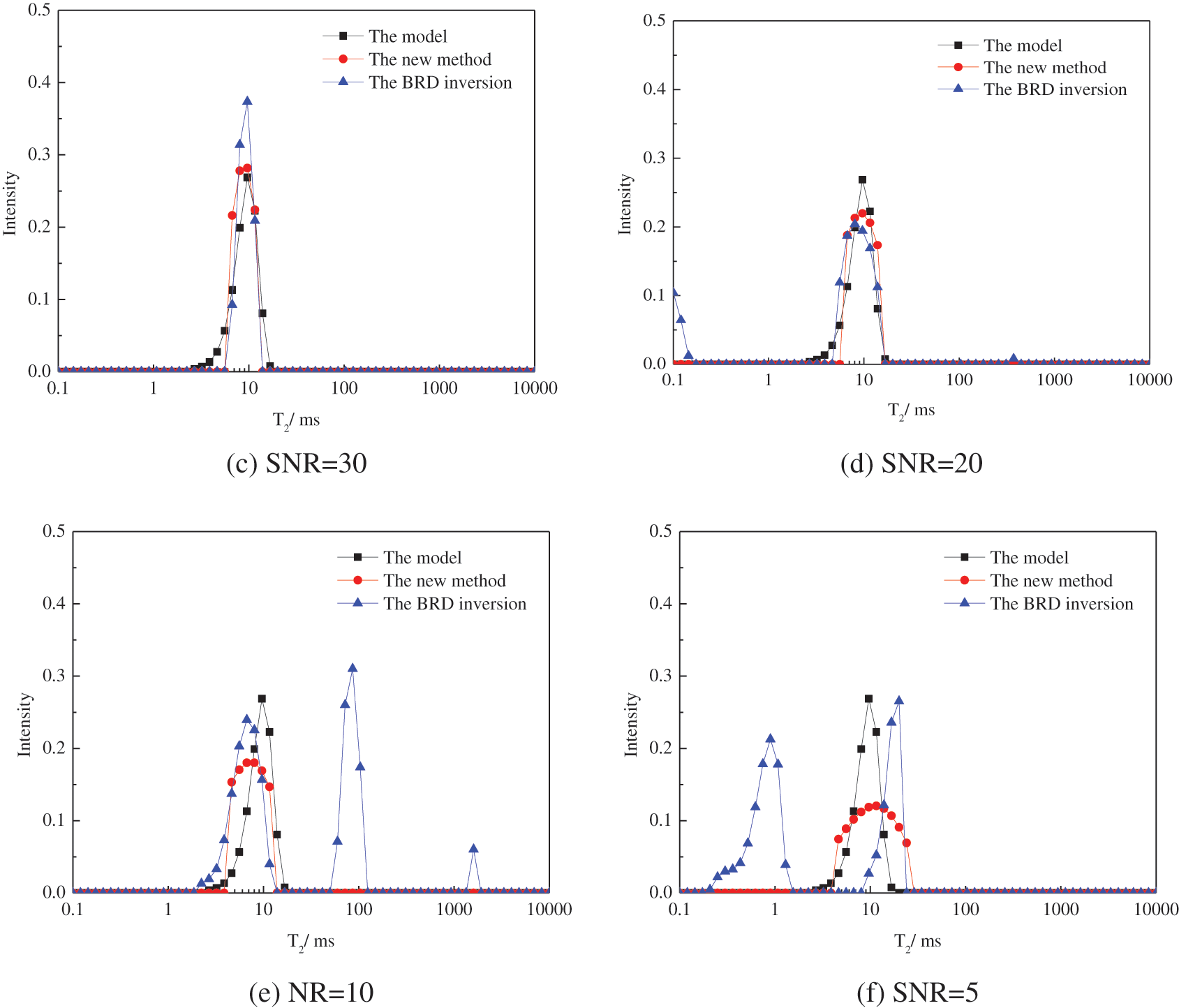
Figure 3: The inverted unimodal spectrums of the signals with different SNRs

4.2 The Bimodal Spectrum

Considering the most common case, the bimodally distributed spectrum is constructed. The positions of the two peaks are 10 ms and 60. Similar to the previous case, Fig. 4 shows the simulated Gaussian’s noises with SNR of 100, 50, 30, 20, 10, and 5. The normalized amplitude of less than 0.001 is dropped and the data is renormalized. The inversion results are shown in Fig. 5. The results show that the inverted spectrum is coherent with the model for echo trains with SNR higher than 30. For echo trains with SNR lower than 20, the deviation between the inverted spectrum and the model increases with the decrease of the SNR. The inversion results are unacceptable when the SNR is less than 10, since the position and the shape are totally changed. The inversion results obtained by the BRD algorithm are similar to the unimodal spectrum.

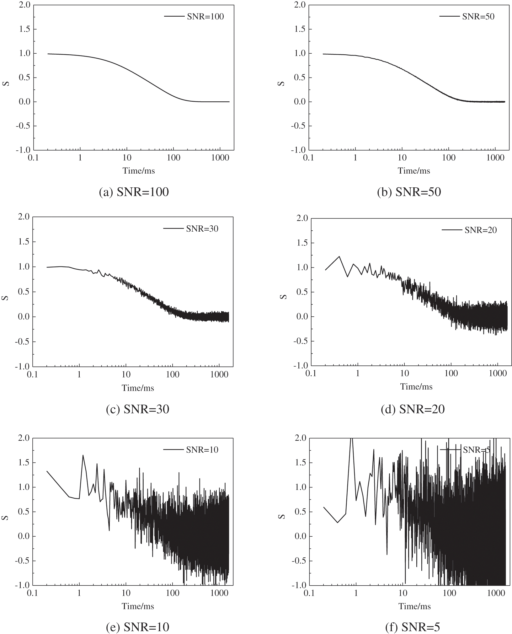
Figure 4: Simulated NMR trains of the bimodal spectrum with different SNRs

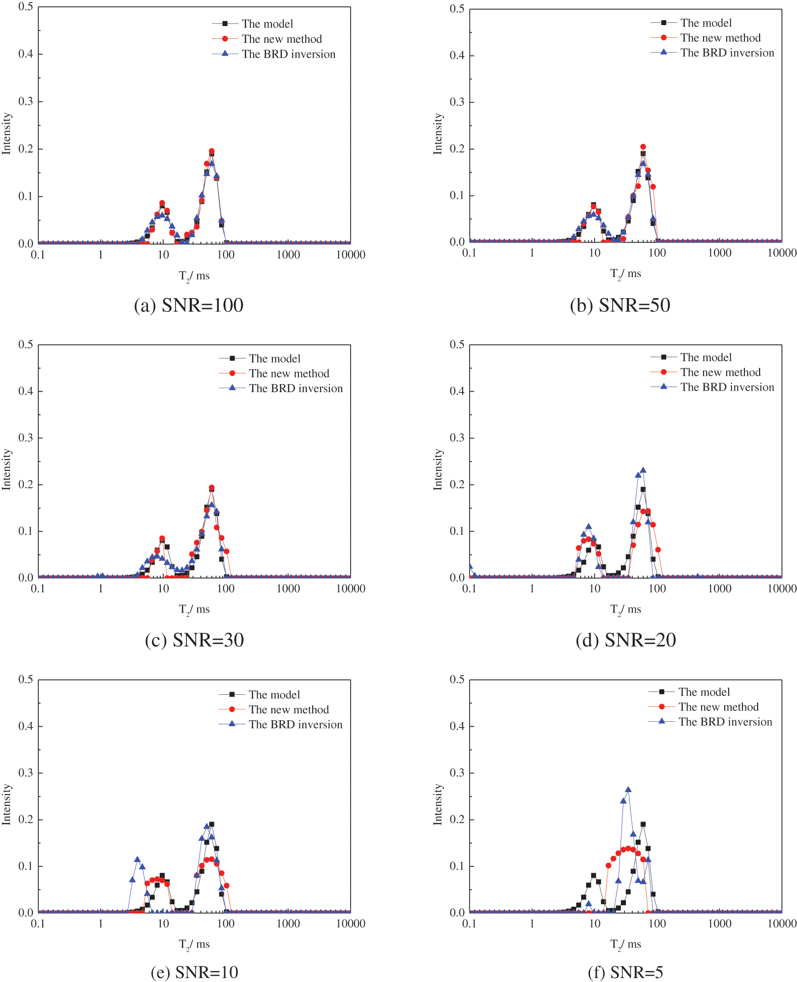
Figure 5: The inverted bimodal spectrums of the signals with different SNRs

Based on the above simulation results, it is concluded that the proposed novel algorithm works very well for the inversion of the T2 spectrum. The proposed algorithm can achieve fast convergence and its inversion results are only slightly influenced by the noise when the SNR is higher than 20.

4.3 Comparison of the Computation Efficiency

Figs. 3 and 5 show the comparisons of the forward model, the inverted spectrums by the new method, and the inverted spectrums by the BRD algorithm. It is obvious that at high SNR (approximately larger than 50), both methods achieve favorable inversion results. However, the inversion results ofthe new method show better performance than the BRD algorithm, when the echo trains contain noises (particularly for the SNR lower than 20). The MSE is defined by:

MSE=1N∑i=1N(yi−inverted−yi−forward)2×10000(22)

where yi−inverted is the amplitude for i-th component of the inverted spectrum; yi−forward is the amplitude for the i-th component of the forward spectrum; N is the number of the components of the spectrum.

Fig. 6 gives the mean square error (MSE) between the forward model and the inversion results for different cases. It is observed that the new method achieves lower MSE than the BRD algorithm, especially for the unimodal distributed spectrum. Fig. 7 compares the time duration between the new method and the BRD inversion for our numerical cases. It is seen that the computation efficiency is greatly enhanced using the new method. Both the results of MSE and the time duration reveal the superiority of the new method.

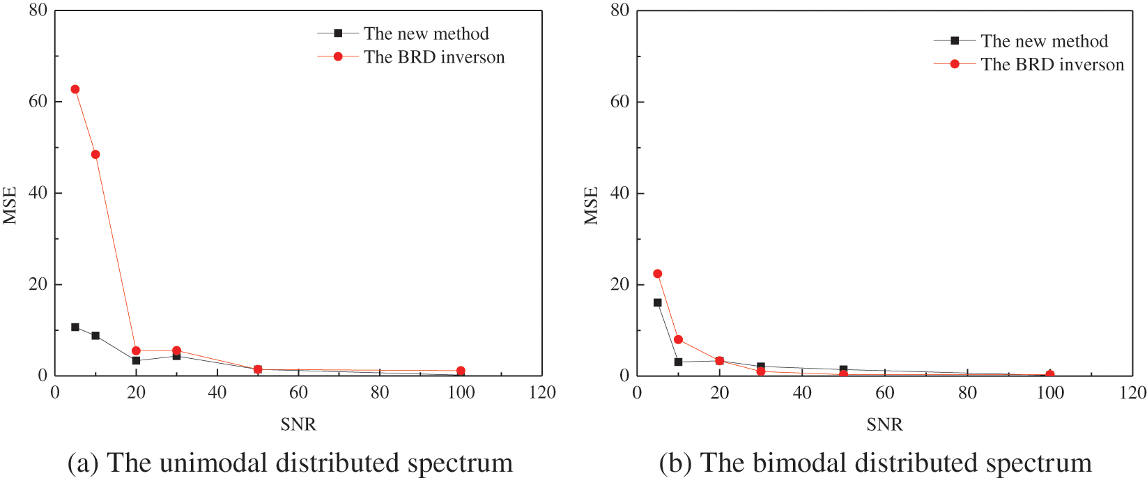
Figure 6: The relationship between the MSE and the SNR at different numerical cases

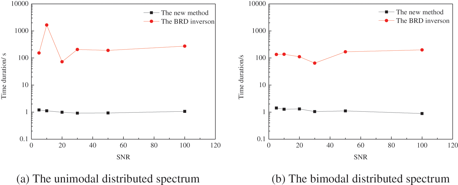
Figure 7: The relationship between the time duration and the SNR at different numerical cases

5  Conclusions

A novel, efficient and accurate algorithm is developed for the inversion of the NMR T2 spectrum. In this method, the empirical TSVD and linearized Bregman iteration are used to enhance the speed and accuracy of the numerical inversion of the NMR T2 spectrum for the first time. The results of the numerical inversion study show that the linearized Bregman iteration can obtain quick and effective performance in the solution of ill-posed and over-determined problems. Moreover, this novel method can work well for data with the SNR higher than 20.

However, much research should be conducted to generalize this method to field applications and experiments. The effects of the iteration parameters and the acquisition parameters on inversion instability are also very important and can be investigated in the future.

Funding Statement: The authors are grateful for the financial support by the National Nature Science Foundation of China (42174142), CNPC Innovation Found (2021DQ02-0402), and National Key Foundation for Exploring Scientific Instrument of China (2013YQ170463).

Conflicts of Interest: The authors declare that they have no conflicts of interest to report regarding the present study.

References

1. Coates, G. R., Xiao, L., Prammer, M. G. (1999). NMR logging principles and applications. Texas, USA: Gulf Publishing Company. [Google Scholar]
2. Dunn, K. J., Bergman, D. J., Latorraca, G. A. (2002). Nuclear magnetic resonance petrophysical and logging application. New York: Elsevier Science, Ltd. [Google Scholar]
3. Ge, X., Liu, J., Fan, Y., Xing, D., Deng, S. et al. (2018). Laboratory investigation into the formation and dissociation process of gas hydrate by low field NMR technique. Journal of Geophysical Research-Solid Earth, 123, 3339–3346. https://doi.org/10.1029/2017JB014705 [Google Scholar] [CrossRef]
4. Zhang, F., Zhang, C. (2021). Evaluating the potential of carbonate sub-facies classification using NMR longitudinal over transverse relaxation time ratio. Advances in Geo-Energy Research, 5(1), 87–103. https://doi.org/10.46690/ager [Google Scholar] [CrossRef]
5. Sun, B., Dunn, K. J. (2004). Methods and limitations of NMR data inversion for fluid typing. Journal of Magnetic Resonance, 169(1), 118–128. https://doi.org/10.1016/j.jmr.2004.04.009 [Google Scholar] [PubMed] [CrossRef]
6. Song, Y. Q. (2013). Magnetic resonance of porous media (MRPMA perspective. Journal of Magnetic Resonance, 229, 12–24. https://doi.org/10.1016/j.jmr.2012.11.010 [Google Scholar] [PubMed] [CrossRef]
7. Tan, M., Zou, Y., Zhou, C. (2015). A new inversion method for (T2, D) 2D NMR logging and fluid typing. Computers and Geosciences, 51, 366–380. https://doi.org/10.1016/j.cageo.2012.07.030 [Google Scholar] [CrossRef]
8. Venkataramanan, L., Song, Y. Q., Hurlimann, M. D. (2002). Solving fredholm integrals of the first kind with tensor product structure in 2 and 2.5 dimensions. IEEE Transactions on Signal Processing, 50(5), 1017–1026. https://doi.org/10.1109/78.995059 [Google Scholar] [CrossRef]
9. Gao, Y., Xiao, L., Zhang, Y., Xie, Q. (2016). The generalized phillips-twomey method for NMR relaxation time inversion. Journal of Magnetic Resonance, 271, 1–6. https://doi.org/10.1016/j.jmr.2016.07.018 [Google Scholar] [PubMed] [CrossRef]
10. Wang, Y., Xia, X., Wang, Y., Wang, L., Hu, W. (2017). Using proper orthogonal decomposition to solve heat transfer process in a flat tube bank fin heat exchanger. Advances in Geo-Energy Research, 1(3), 158–170. https://doi.org/10.26804/ager [Google Scholar] [CrossRef]
11. Zhou, X., Su, G., Wang, L., Nie, S., Ge, X. (2017). The inversion of 2D NMR relaxometry data using L1 regularization. Journal of Magnetic Resonance, 275, 46–54. https://doi.org/10.1016/j.jmr.2016.12.003 [Google Scholar] [PubMed] [CrossRef]
12. Day, I. J. (2011). On the inversion of diffusion NMR data: Tikhonov regularization and optimal choice of the regularization parameter. Journal of Magnetic Resonance, 211, 178–185. https://doi.org/10.1016/j.jmr.2011.05.014 [Google Scholar] [PubMed] [CrossRef]
13. Bortolott, V., Brown, R. J. S., Fantazzini, P., Landi, G., Zama, F. (2018). I2DUPEN: Improved 2DUPEN algorithm for inversion of two dimensional NMR data. Microporous and Mesoporous Materials, 269, 195–198. https://doi.org/10.1016/j.micromeso.2017.04.038 [Google Scholar] [CrossRef]
14. Berman, P., Levi, O., Parmet, Y., Saunders, M., Wiesman, Z. (2013). Laplace inversion of low-resolution NMR relaxometry data using sparse representation methods. Concepts in Magnetic Resonance Part A, 42(3), 72–88. https://doi.org/10.1002/cmr.a.21263 [Google Scholar] [PubMed] [CrossRef]
15. Guo, J., Xie, R., Xiao, L., Jin, G., Gao, L. (2019). Nuclear magnetic resonance T1–T2 inversion with double objective functions. Journal of Magnetic Resonance, 308, 106562. https://doi.org/10.1016/j.jmr.2019.07.049 [Google Scholar] [PubMed] [CrossRef]
16. Guo, J., Xie, R., Liu, M. (2018). A robust algorithm for 2-D NMR diffusion–Relaxation spectra inversion. IEEE Geoscience and Remote Sensing Letters, 15(10), 1545–1549. https://doi.org/10.1109/LGRS.2018.2853667 [Google Scholar] [CrossRef]
17. Bortolotti, V., Landi, G., Zama, F. (2021). 2DNMR data inversion using locally adapted multi-penalty regularization. Computational Geosciences, 25(3), 1215–1228. https://doi.org/10.1007/s10596-021-10049-y [Google Scholar] [CrossRef]
18. Yin, W., Osher, S., Goldfarb, D., Darbon, J. (2008). Bregman iterative algorithms for l1-minimization with applications to compressed sensing. SIAM Journal on Imaging Sciences, 1(1), 143–168. https://doi.org/10.1137/070703983 [Google Scholar] [CrossRef]
19. Chai, X., Tang, G., Peng, R., Liu, S. (2018). The linearized bregman method for frugal full-waveform inversion with compressive sensing and sparsity-promoting. Pure and Applied Geophysics, 175, 1085–1101. https://doi.org/10.1007/s00024-017-1734-4 [Google Scholar] [CrossRef]
20. Gou, F. Y., Liu, C., Liu, Y., Feng, X., Cui, F. Z. (2014). Complex seismic wavefield interpolation based on the bregman iteration method in the sparse transform domain. Applied Geophysics, 11(3), 277–288. https://doi.org/10.1007/s11770-014-0443-3 [Google Scholar] [CrossRef]
21. Cai, J. F., Osher, S., Shen, Z. (2009). Convergence of the linearized bregman iteration for l1-norm minimization. Mathematics of Computation, 78, 2127–2136. https://doi.org/10.1090/S0025-5718-09-02242-X [Google Scholar] [CrossRef]
22. Bush, J. (2011). Bregman algorithms. Santa Barbara: University of California. [Google Scholar]
23. Arns, C. H., Washburn, K. E., Callaghan, P. T. (2007). Multidimensional NMR inverse laplace spectroscopy in petrophysics. Petrophysics, 48(5), 380–392. [Google Scholar]
24. Tan, M. J., Zou, Y. L. (2012). A hybrid inversion method of (T2, D) 2D NMR logging and observation parameters effects. Chinese Journal of Geophysics-Chinese Edition, 55(2), 683–692. [Google Scholar]
25. Fan, Y. R., Wu, F., Li, H., Huo, N. N., Wang, Y. S. et al. (2015). A modified design of pulse sequence and inversion method for DT-2 two-dimensional NMR. Acta Physica Sinica, 64(9), 099301. [Google Scholar]
26. Zou, Y. L., Xie, R. H., Arad, A. (2016). Numerical estimation of choice of the regularization parameter for NMR T2 inversion. Petroleum Science, 13, 237–246. https://doi.org/10.1007/s12182-016-0093-6 [Google Scholar] [CrossRef]
27. Zhou, X. L., Nie, S. D., Wang, Y. J., Zhang, Y. L., Yang, P. Q. (2013). An iterative truncated singular value decomposition (TSVD)-based inversion method for 2D NMR. Chinese Journal of Magnetic Resonance, 30(4), 541–551 (in Chinese). [Google Scholar]
28. Jiang, Z. M., Wang, W. M. (2013). A method of choosing the optimal number of singular values in the inverse laplace transform for the two-dimensional NMR distribution function. Chinese Physics Letters, 30(1), 010201. https://doi.org/10.1088/0256-307X/30/1/010201 [Google Scholar] [CrossRef]
Cite This Article
Copyright © 2023 The Author(s). Published by Tech Science Press.
This work is licensed under a Creative Commons Attribution 4.0 International License , which permits unrestricted use, distribution, and reproduction in any medium, provided the original work is properly cited.
Downloads
Citation Tools