Research on Short-Term Load Forecasting of Distribution Stations Based on the Clustering Improvement Fuzzy Time Series Algorithm

1  Introduction

Power demand forecasting plays an important role in modern power system research. Accurate prediction of power load in different periods in the future will improve the management level of the power system [1,2]. According to the forecasting time, load forecasting can be divided into three main forms: short term, long term and super long term. Short-term load forecasting is the prediction of power load in the next few minutes to a week. Accurate short-term load forecasting will help to formulate a reasonable power production plan. It also can avoid excessive waste of power resources and improve the economic benefits of the power system [3–5]. Short-term load forecasting methods mainly fall into two categories: statistical methods and machine learning methods. Statistical methods mainly include regression analysis, time series, Markov chain, etc. Machine learning methods mainly include support vector machines (SVM), artificial neural networks, etc. [6–8].

In the study of statistical methods, short-term load forecasting was performed by using an improved Gaussian process regression model with multi-core covariance, and the interval prediction results at a certain confidence level were obtained [9]. The gray time series modified by Markov was used to predict the power load trend, and the prediction accuracy was higher than that of single algorithm models such as time series and Markov chain [10]. A blind Kalman filter algorithm was proposed for short-term load forecasting, which has great advantages in load profile analysis and peak load forecasting by predicting unknown matrix and state alternation estimation [11]. The mixed random forest algorithm and mean generating functions were used to form a hybrid short-term load forecasting model, which has better prediction accuracy for peak and valley conditions with the large change of load data [12]. An adaptive hybrid fractal model was proposed for power system short-term load forecasting, composed of composite linear fractal difference function, iterative learning and optimization algorithm, and has higher accuracy than commonly used time series methods [13]. A load forecasting method based on the combination of multiple phase space reconstruction (MPSR) and support vector regression (SVR) was proposed, which takes into account the coupling relationship between multiple energy loads and has high prediction efficiency and accuracy [14]. A seasonal autoregressive integrated moving average and variance-covariance prediction method was proposed, which considered the interaction of multiple performance indicators and had high prediction accuracy [15].

In the study of machine learning methods, the joint learning method based on recurrent neural networks was used to predict short-term load changes, which has a good prediction effect [16]. The prediction interval of the neural network was used to construct a lower bound estimation method, which can quantify the potential uncertainty factors related to prediction and predict the load change trend with high accuracy in a short time [17]. The two-stage attention mechanism based on the long-term and short-term memory (LSTM) neural network was introduced for the probability prediction of short-term regional load, and the prediction model has higher accuracy and generalization ability [18]. A time convolutional neural network that integrated channel and time attention mechanism was proposed for short-term load forecasting of the power system, which effectively expressed the nonlinear relationship between meteorological factors and power load [19]. In [20], a holographic integrated forecasting method for short-term power load was proposed, which integrates multi-category and multi-state load information into four levels (data set, sampling space, prediction model and decision), which can comprehensively integrate information throughout the whole life cycle of the forecasting process and greatly improve the effect of short-term load forecasting. In [21], Box-Cox conversion processing and parameter fitting of Copula model were carried out for loaded load data, and a data-driven deep confidence network was proposed to predict the hourly load of the power system. In [22], nonlinear exogenous recurrent neural network (NARX), Elman neural network and autoregressive moving average (ARMA) were used for short-term load forecasting, and it was found that the average absolute percentage errors of NARX, Elman and ARMA were 5.53%, 3.42% and 10.28%, respectively. In [23], a personalized federated learning method was proposed, with high prediction accuracy in individual consumer load forecasting. In addition to the above literature, An et al. [24–27] also adopted different methods to study load forecasting of the power system.

The statistical method is simple in principle and fast in the calculation, but it has limited ability to deal with nonlinear variables. While the machine learning method can approach the nonlinear function relationship with arbitrary precision in principle, it is difficult to mine the timing characteristics between data [28,29]. How to integrate intelligent algorithms into typical time series prediction methods to improve the processing ability of its nonlinear function is worthy of in-depth research. Time series analysis includes two parts: time series modeling and time series forecasting. Modeling is the rational cognition of the internal development law of things, while forecasting is the specific performance of future development trend based on the model. The classical time series analysis method can deal with most realistic problems, but it cannot deal with the imprecise, incomplete or fuzzy realistic problems. For example, the change of power load is often expressed as “sudden increase, sudden decrease, steady” and other language variables. Although these phenomena can be described with accurate numerical values, it is very difficult to obtain historical data, similar to the above vague or incomplete data are more. In this case, fuzzy time series expressed by linguistic variables can be used for prediction.

At present, the theoretical research of fuzzy time series mainly focuses on the reasonable division of fuzzy interval. Fuzzy interval has a great influence on the calculation process and prediction accuracy of the model, which is the basis of establishing fuzzy time series prediction model. In [30], the concept of fuzzy time series was put forward, which was a pioneer in the theory and application of fuzzy time series. In [31,32], the maximum and minimum values of the sample data were rounded as the domain of the model, and then the fixed interval length was selected to divide the domain equally. The membership function setting of this method was simple and the calculation speed was fast, but the fuzzy set corresponding to the interval was not accurate, which led to the low prediction accuracy. In [33,34], the distribution characteristics of sample data were used to divide the domain. The interval with dense sample data was reduced, and the interval with sparse sample data was expanded. The interval division based on statistical characteristics was more reasonable, and the prediction accuracy of the model was improved to a certain extent. In [35–37], neural networks and optimization algorithms were used to divide the domain, aiming to find the optimal number and length of intervals. The prediction accuracy of this method was greatly improved, but the divided interval was difficult to be interpreted in natural language, which weakened the advantage of fuzzy theory in the application of time series prediction. Using the clustering algorithm to cluster the sample data, and taking the clustering results as the basis for domain division, each interval represents a clearer practical significance, and the prediction effect is also very accurate, so this kind of algorithm is very meaningful.

Power load forecasting is the basis of power system operation management and real-time regulation. It is an important link in the reform of the electric power system and the transformation of energy structure to constantly improve the power load forecasting technology and seek a more accurate load forecasting model. It is helpful for decision makers to make reasonable power grid dispatching plan and maintain the safe and economic operation of the power grid. Combined with the scenario of short-term load forecasting in the distribution station, this paper focuses on the prediction performance of fuzzy time series and its improved algorithm. The innovation points of this paper are as follows:

1.    The typical fuzzy time series can predict the time series data containing fuzzy information or incomplete information, and the improved fuzzy time series still has this feature.

2.    The typical fuzzy time series adopts the principle of equal division of the domain. While the improved fuzzy time series divides the domain according to the probability distribution characteristics of the data, and the division of the domain is more reasonable.

3.    Fuzzy time series represented by high-order fuzzy relations can better fit the nonlinear relationship between data. This paper presents a concrete design method for the third order fuzzy time series.

4.    The prediction algorithm proposed in this paper can be applied to other fields, such as traffic flow and weather, etc. The prediction accuracy of the algorithm is high, and the algorithm is universal.

2  K-Means Clustering and Fuzzy Time Series

2.1 K-Means Clustering Method

Clustering is the process of classifying and organizing samples with similar characteristics in a data set. As one of the most famous partition clustering algorithms, K-means clustering is widely used due to its simplicity and efficiency. It is a clustering analysis algorithm based on iterative solution process [38,39]. The algorithm steps are as follows:

1)   k samples are randomly selected from the data set containing n samples as the initial clustering center Ci (i = 1, 2, …, k).

2)   According to the initial value of each cluster center, the absolute distance Dk=|Xk−Ci| from each sample Xk(k=1,2,…,n) to the cluster center Ci was calculated. Then the samples are divided into class clusters Li (i = 1, 2, …, Ni) according to the shortest distance, Ni is the number of samples contained in each cluster.

3)   Calculating the mean of each cluster Ci=∑Xk∈LiXk/Ni, which is used as the clustering center after the algorithm is updated.

4)   Repeating Steps 2 and 3 until all samples cannot be redistributed.

2.2 Fuzzy Time Series

Fuzzy time series analysis refers to the use of fuzzy mathematics theory to study the deep nonlinear relationship contained in the time series containing fuzzy or uncertain information. The relevant definitions involved are as follows [40–42]:

Definition 1: Let U be the domain of time series, and divide the domain into n ordered subintervals, i.e., U = {u1, u2, …, un}, then the fuzzy set A defined on domain U can be expressed as:

A=fA(u1)/u1+fA(u2)/u2+⋯+fA(un)/un(1)

where fA(⋅) is membership function, fA(ui) is the membership of ui to A, fA(ui)ϵ[0,1],i=1,2,…,n.

Definition 2: Let X(t)(t=1,2,…,n) be a subset of the real number set R, and fi(t)(i=1,2,…,n) be a fuzzy set defined on the domain X(t). If F(t)is a set composed of fi(t), then F(t) is a fuzzy time series defined on X(t).

Definition 3: If F(t−1)=Ai,F(t)=Aj, the fuzzy logic relationship (FLR) can be expressed as

Ai→Aj, Ai is the left components of FLR, Aj is the right components of FLR, and R(t,t−1) is the fuzzy logic relationship from F(t−1) to F(t), then the first-order model can be expressed as:

F(t)=F(t−1)∘R(t,t−1)(2)

where ∘ represents compositional operation. Similarly, the n-order model of F(t) can be obtained, that is, the relationship between F(t) and F(t−1),F(t−2),⋯,F(t−n), which is expressed as follows:

F(t)=F(t−1)∘Rn(t,t−1)(3)

Definition 4: If the left components of multiple fuzzy logic relationships are the same, but the right components are different, these fuzzy logic relationships can be combined into a relationship, that is, a fuzzy logic relationship group.

Ai→Aj1,Aj2,⋯(4)

3  Fuzzy Time Series Prediction Model

3.1 Typical Fuzzy Time Series Prediction (FTS)

Typical fuzzy time series prediction includes the following steps:

(1) Based on historical data, the domain is determined. Let X={x1,x2,⋯,xn} be a time series, then the domain U can be defined as:

U=[Dmin−d1,Dmax+d2](5)

where Dmin and Dmax are the minimum and maximum values in X, and d1 and d2 are two customized real numbers.

(2) Dividing the domain equally to form multiple numerical subintervals. It is worth noting that too large or too small subinterval range will have a certain impact on the final prediction results, and its range must be selected reasonably.

(3) Fuzzy sets are defined to fuzzify the data. Suppose that there are m subintervals formed after the domain is divided equally, then the corresponding fuzzy set is defined as A={A1,A2,⋯,Am}, and Ai is the language variable of A. Fuzzify the historical data according to the triangular membership function, and the process is as follows:

A1=f11x1+f12x2+⋯+f1nxn

A2=f21x1+f22x2+⋯+f2nxn(6)

⋯

An=fn1x1+fn2x2+⋯+fnnxn

(4) Establish fuzzy logic relation and determine fuzzy relation matrix. If Ai is the fuzzy membership of data i and Aj is the fuzzy membership of data j, then the fuzzy logic relationship can be expressed as Ai→Aj. Thus, the fuzzy logic relation Ri(i=1,2,⋯) between the values of each fuzzy time series can be written, and the fuzzy relation matrix can be obtained by combining the fuzzy logic relations R=R1∪R2⋯.

(5) Defuzzification and prediction. According to the established fuzzy relation, the time series data can be predicted. During the prediction, the fuzzy quantity needs to be de fuzzified to obtain an accurate numerical quantity. The defuzzification method adopts the weighted average method, as shown in Eq. (7).

Y=∑i=1pcimi/p(7)

where p is the number of fuzzy relations corresponding to the fuzzy set Ai obtained by fuzzifying the data xi, ci is the weight, and mi is the intermediate value of the interval ui corresponding to the fuzzy set Ai.

3.2 Improved Fuzzy Time Series Prediction (IFTS)

In the typical fuzzy time series prediction method, the equal division principle is used to divide the domain. However, from the probability distribution characteristics of the data, it can be seen that the data distribution is generally uneven. At this time, the equal division principle is unreasonable to divide the domain. Therefore, this paper considers the cluster centers as the basis for domain division, and the resulting subinterval will be more reasonable and have data similarity. The principles of domain division are as follows:

u1=[xmin−d1 l1](8)

un=[lc xmax+d2](9)

ui=[lc−1lc](10)

where ui(i=1,2,⋯,n) is each subinterval, lj(j=1,2,⋯,c) is the average value of cluster centers, dk(k=1,2) is the minimum difference of cluster centers, and the calculation formulas of lj and dk are as follows:

dk=min[ci−1−ci](11)

lj=(ci+1+ci)/2(12)

where ci(i=1,2,⋯,k) is cluster center.

In addition, the typical fuzzy time series prediction method often uses the first-order fuzzy relationship, but the higher-order fuzzy relationship can better reflect the nonlinear function relationship between data. Therefore, this paper adopts the third-order fuzzy relation, that is, the data at t − 2, t − 1 and t time are used to predict the data at t + 1 time. The prediction process is as follows:

Di=||Xi−Xi−1|−|Xi−1−Xi−2||(13)

Zi=Xi+Di/2(14)

ZZi=Xi−Di/2(15)

Yi=Xi+Di(16)

YYi=Xi−Di(17)

Fi+1=(P+M[Ai∗])/(S+1)(18)

where Di, Zi, ZZi, Yi and YYi are the set calculation variables, Xi represents the data at time i, Fi+1 represents the predicted value at time i + 1, P, S are temporary variables for data accumulation, with values as shown in Table 1, [Ai∗] is the interval uj with membership of 1 in the fuzzy set Ai, and M[Ai∗] is the median value of interval uj.

3.3 Evaluation of Prediction Accuracy

The prediction accuracy of time series is often tested by residual size. In this paper, four indexes including mean square error (MSE), root mean square error (RMSE), mean relative error (MRE) and efficiency coefficient NS are selected to evaluate the prediction accuracy of the model, which can be expressed by the following formulas:

MSE=∑i=1n(yi−y^i)2n(19)

RMSE=1/n∑i=1n(yi−y^i)2(20)

MRE=1n∑i=1n|yi−y^iyi|×100%(21)

NS=1−∑i=1n(yi−y^i)2∑i=1n(yi−y¯)2(22)

where yi is the measured value, y^i is the predicted value, y¯ is the average value of the measured value, and n is the numbers of data. When EMS = 0, RMSE = 0, MARE = 0, NS = 1, the model fitting effect is the best.

In addition, it is pointed out in [43] that the modified Diebold-Mariano test statistic (MDM) can be used to evaluate whether the loss function between different models is statistically significant. If the loss function error of each model is statistically different, the prediction ability of each model is obviously different.

Assuming that the sequence formed from the measured values is {ft} and the sequence formed from the predicted values is {f^t}, the prediction error of the model can be expressed as Eq. (23).

et=ft−f^t(23)

The loss function at time t can be expressed as Eq. (24).

Loss=L(et)=L(ft,f^t)(24)

where L is the sign of the loss function.

The prediction results of different models are different, resulting in different prediction errors and loss function values. When the performance of the two prediction models is compared, the H0 hypothesis theory can be used.

H0: E(dt)=0(25)

dt=L(e1t)−L(e2t)(26)

where e1t is the prediction error of model 1, e2t is the prediction error of model 2. It is worth noting that the two models satisfying the H0 hypothesis will have the same predictive performance.

MDM is an important indicator to evaluate the predictive ability of a model and can be expressed as follows:

MDM=y¯w^n+1−2h+h(h−1)n(27)

w^2=r^0+2∑j=1h−1r^j(28)

r^j=1n∑i=j+1n(yi−y¯)(yi−j−y¯)(29)

where h is the number of steps before prediction.

4  Application Case Analysis

4.1 Analysis of Statistical Characteristic of Power Load Measured Value

The power load data in this paper comes from a distribution station of a city in Zhejiang Province, China. It is the real load data obtained based on the intelligent meter advanced measurement system. Sampling is conducted every 15 min to obtain 35,040 load data in 2021. According to the above data, the correlation statistical analysis of power load can be carried out by Matlab/Simulink software and its programming. Fig. 1a shows the change trend of power load in 2021, Fig. 1b shows the partial diagram of power load at a certain stage in 2021, and Fig. 2 shows the frequency distribution histogram of power load in different intervals.

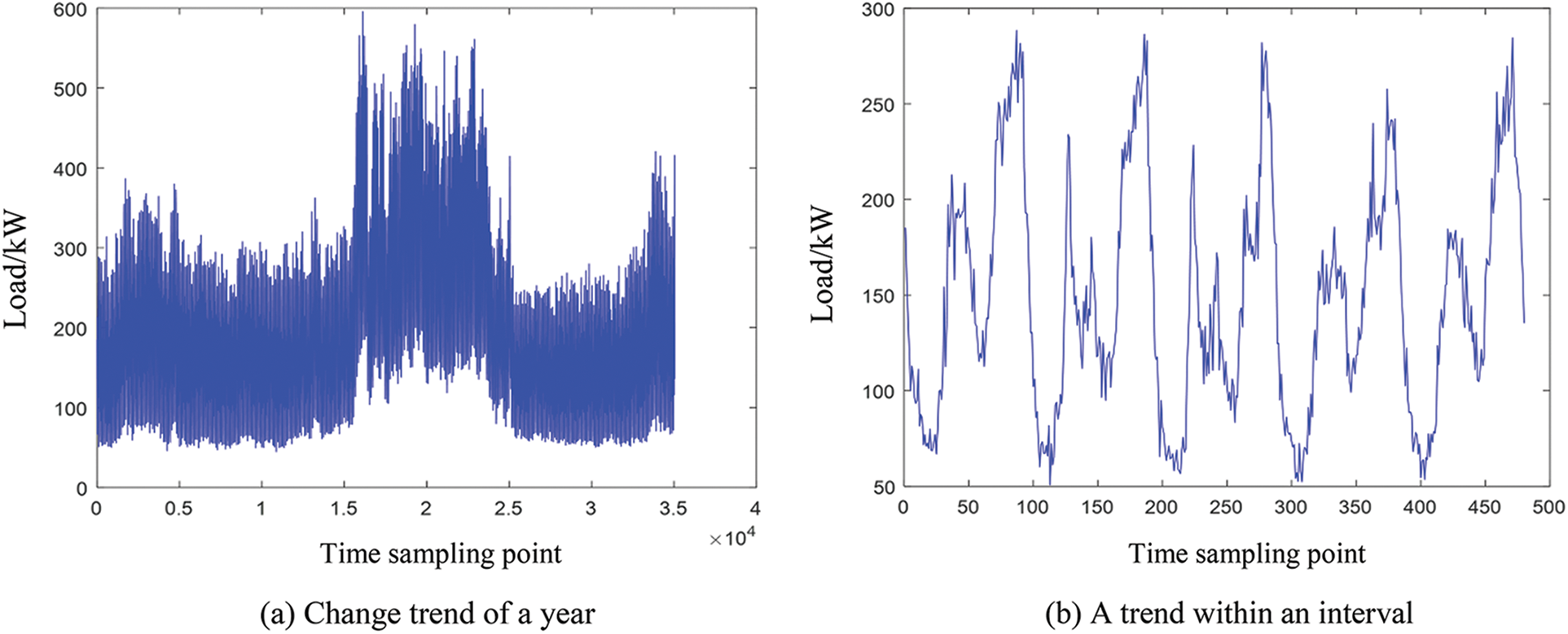
Figure 1: Variation trend of power load in 2021

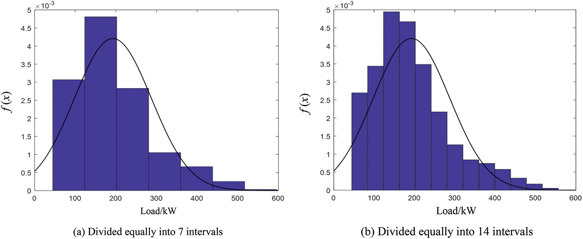
Figure 2: Frequency distribution histogram of power load

As can be seen from Fig. 1a, the change of power load shows strong nonlinearity and seasonality, that is, the power load in summer is significantly higher than that in other seasons, which is basically consistent with the power load in Southern China. It can be seen from Fig. 1b that the short-term change of power load has obvious periodicity. The periodicity of short-term load can be used to predict the short-term load change in the future, so as to formulate a reasonable power grid dispatching plan.

It can be seen from Fig. 2 that the power load frequency in different intervals is different, and the smaller the interval, the better the probability density curve fitting, but the interval has certain limitations. This also shows that it is very necessary to divide the fuzzy interval reasonably when using fuzzy time series to predict power load.

4.2 Analysis of Power Load Forecasting Results

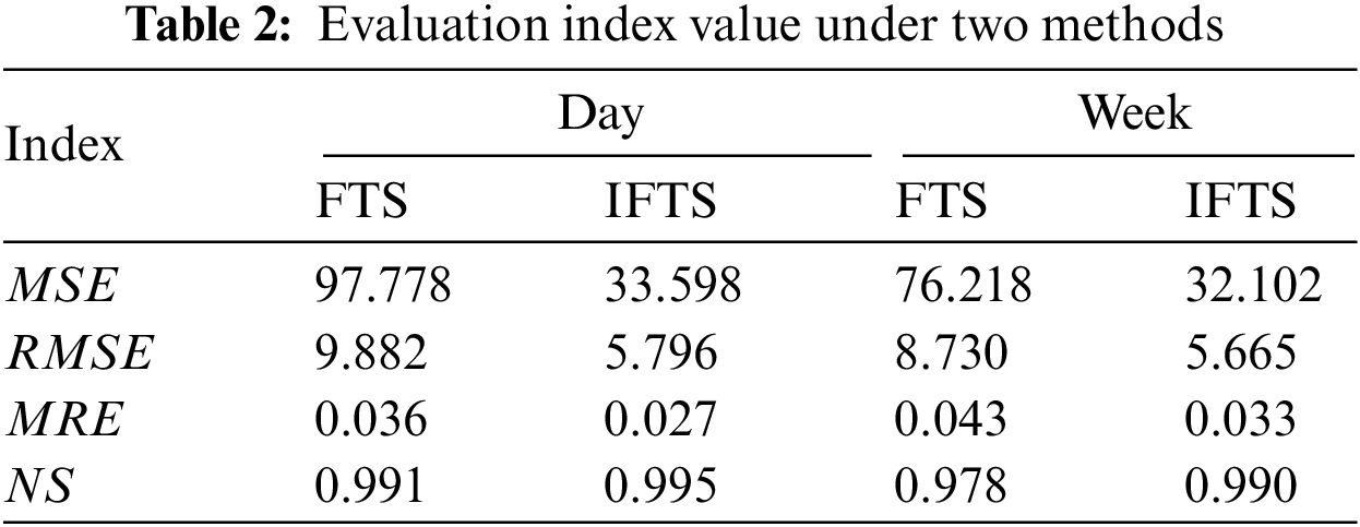
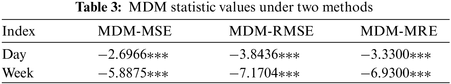
The simulation platform uses Matlab/Simulink software, and the programming language uses m language. Based on this, the relevant algorithm programs are written in this paper. The load forecasting results of one day and one week are observed respectively, and the short-term power load forecasting results under different algorithms are compared and analyzed. Fig. 3 shows the prediction results and errors under the typical fuzzy time series in a day, Fig. 4 shows the prediction results and errors under the clustering improved fuzzy time series in a day. Fig. 5 shows the prediction results and errors under the typical fuzzy time series in a week, Fig. 6 shows the prediction results and errors under the clustering improved fuzzy time series in a week. Table 2 shows the MSE, RMSE, MRE and NS of the two algorithms at different sampling times. The loss functions used in the MDM test follow the metric functions defined earlier in this paper, namely mean square error (MSE), root mean square error (RMSE), and mean relative error (MRE). MDM statistic values of the two algorithms under different sampling times are shown in Table 3.

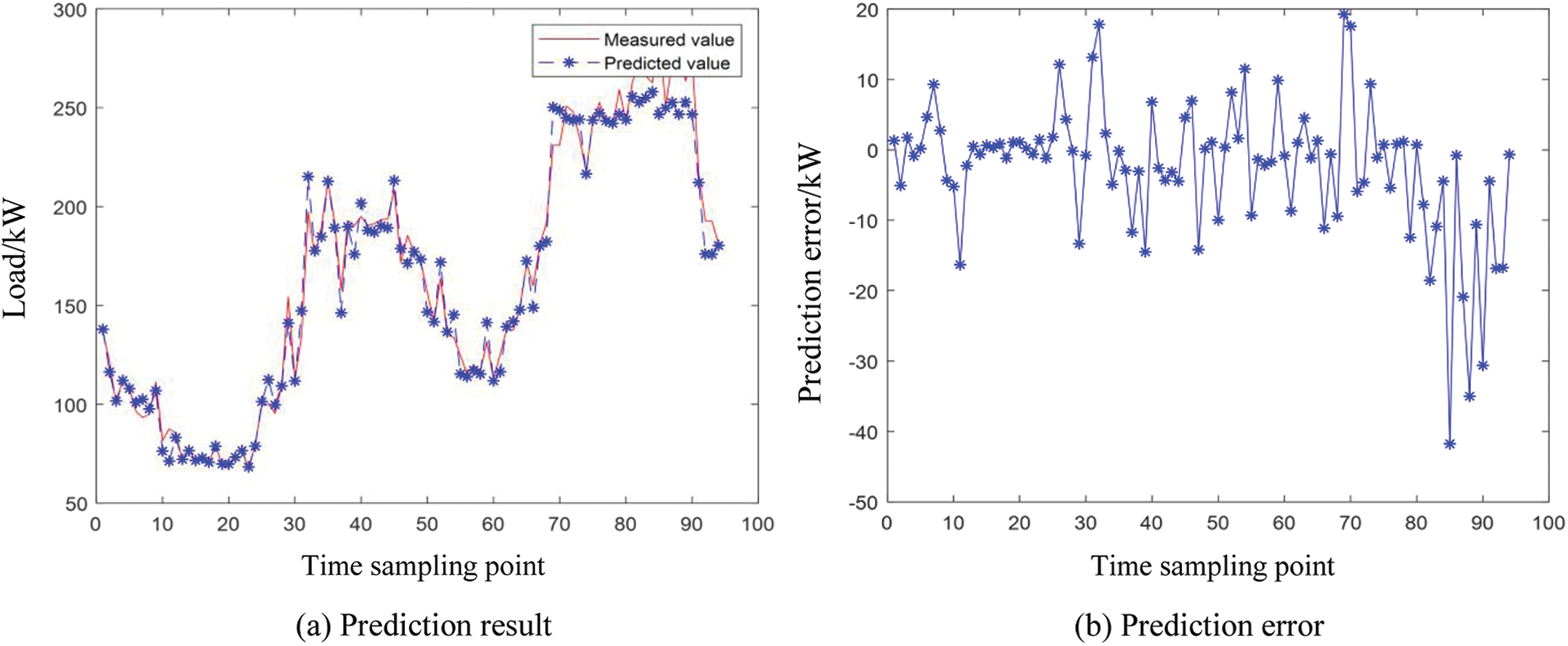
Figure 3: FTS prediction results and errors in a day

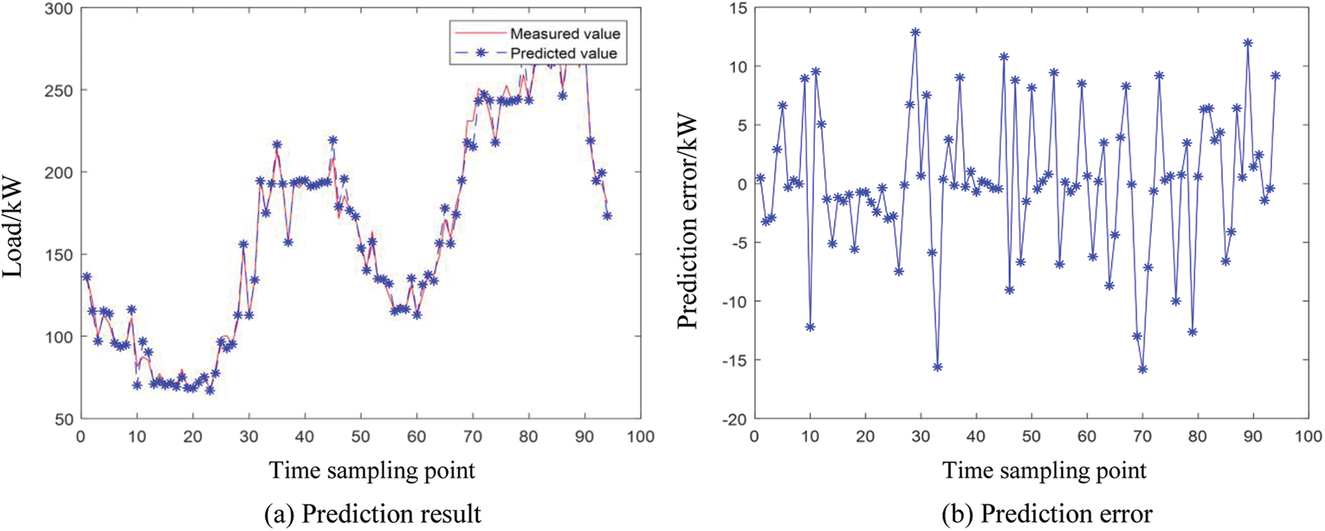
Figure 4: IFTS prediction results and errors in a day

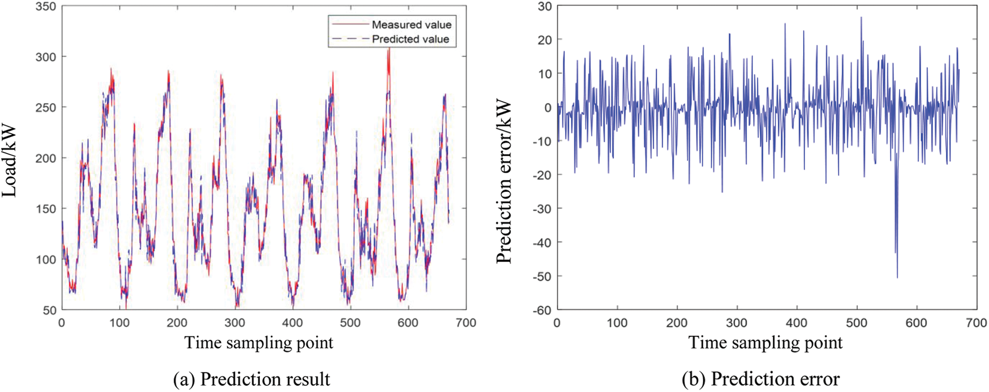
Figure 5: FTS prediction results and errors in a week

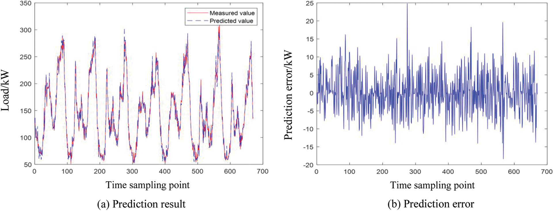
Figure 6: IFTS prediction results and errors in a week

It can be seen from Fig. 3 that the daily power load prediction error of typical fuzzy time series is between −50 and 20. As can be seen from Fig. 4, the prediction error of daily power load in clustering improved fuzzy time series is between −20 and 15. It shows that the prediction algorithm designed in this paper is reasonable and can improve the prediction accuracy to a certain extent.

It can be seen from Fig. 5 that the weekly power load prediction error of typical fuzzy time series is between −50 and 30. As can be seen from Fig. 6, the prediction error of weekly power load in clustering improved fuzzy time series is between −20 and 25. Both algorithms can effectively predict the trend of power load change on a one-week time scale, but the prediction accuracy of the clustering improved fuzzy time series is higher than that of the typical fuzzy time series, indicating that the proposed algorithm in this paper is reasonable and effective.

It can be seen from Table 2 that the evaluation indexes MSE, RMSE and MRE of the fuzzy time series prediction method improved by clustering are less than those of the typical fuzzy time series prediction method. The evaluation index NS of the fuzzy time series prediction method improved by clustering is better than the typical fuzzy time series prediction method, which further reflects the accuracy of the prediction results.

In Table 3, *, ** and *** indicate that the null hypothesis is rejected at the significance level of 10%, 5% and 1%, respectively, that is, * represents p < 0.1, ** represents p < 0.05, *** represents p < 0.01.

As can be seen from Table 3, at the time scale of one day and one week, various MDM statistical values between FTS and IFTS models do not accept the null hypothesis at the significance level of 1%. It indicates that the prediction accuracy of FTS and IFTS models is significantly different. Furthermore, the IFTS model can improve the prediction accuracy, but there is still much room for improvement. In the subsequent study, other clustering algorithms will be considered to further improve the prediction performance of fuzzy time series.

4.3 Comparison with Other Load Forecasting Methods

Typical time series forecasting methods include moving average model (MA), autoregressive model (AR), autoregressive moving average model (ARMA) and so on. Fuzzy time series prediction method is a kind of combined form, and its performance is generally better than that of a single time series prediction method, so it is not compared with this kind of algorithm.

There are two parts that affect the prediction performance of fuzzy time series: 1. The division criterion of the domain; 2. Defuzzification method. In [44–46], the central method is used as the main method of defuzzification, so the comparison experiment with this kind of algorithm will be more practical significance. Figs. 7 and 8 show the load forecasting results and errors of fuzzy time series based on the central defuzzification method (CD-FTS) on the time scale of one day and one week.

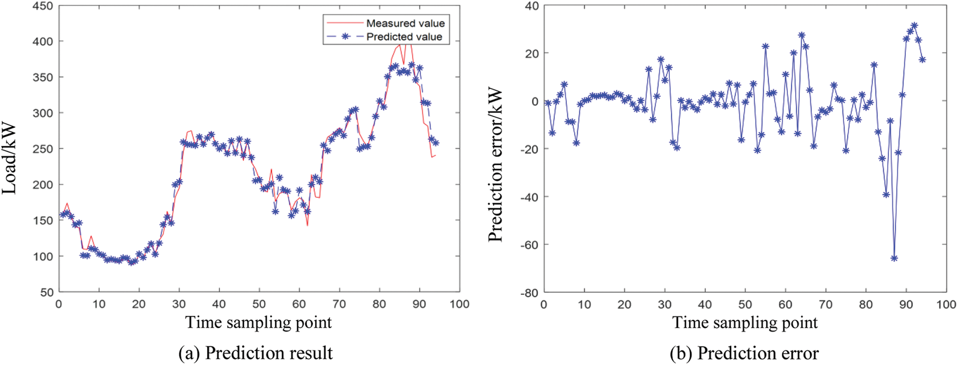
Figure 7: CD-FTS prediction results and errors in a day

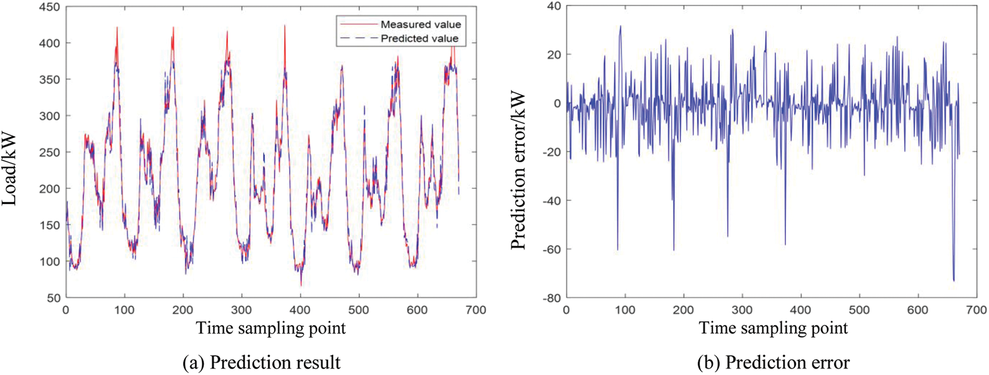
Figure 8: CD-FTS prediction results and errors in a week

It can be seen from Figs. 7 and 8 that the CD-FTS method can effectively predict the short-term variation trend of load, and the prediction error range on the time scale of one day and one week is [−80, 40]. The prediction error of the CD-FTS is much larger than that of the IFTS, which further demonstrates the superiority of the proposed algorithm in this paper.

5  Conclusion

This paper presents a fuzzy time series prediction method based on K-means clustering and applies it to the actual case of short-term power load forecasting in distribution stations. The following conclusions are obtained through Matlab/Simulink simulation case analysis: (1) The fuzzy time series prediction method improved by clustering has a more reasonable division of the fuzzy theory domain. (2) The fuzzy time series expressed by higher-order fuzzy relation can better fit the nonlinear relation between data. (3) The load forecasting evaluation indexes MSE/RMSE/MRE/NS of typical fuzzy time series on the time scale of one day are 97.778/9.882/0.036/0.991. The corresponding values of the improved fuzzy time series are 33.598/5.796/0027/0.995. The MSE/RMSE/MRE value of the typical fuzzy time series is greater than the corresponding value of the improved fuzzy time series, while the NS value of the typical fuzzy time series is less than the corresponding value of the improved fuzzy time series. It shows that the improved fuzzy time series method can improve the forecasting accuracy of power load. (4) Similarly, the load forecasting evaluation indexes MSE/RMSE/MRE of the typical fuzzy time series is larger than the corresponding value of the improved fuzzy time series in the one-week time scale, while the NS value is small. It further shows that the design of the improved fuzzy time series algorithm is reasonable and effective. (5) The null hypothesis is not accepted for various MDM statistic values between fuzzy time series and improved fuzzy time series at the 1% level of significance. The MDM values of the two algorithms are different, indicating that their prediction performance is different.

In addition, the prediction algorithm proposed in this paper can be applied to prediction research in other fields, and it has certain universality. However, the factors affecting power load change are not single, such as temperature, humidity and other environmental factors. Whether the clustering improved fuzzy time series prediction method proposed in this paper is still accurate in power load prediction under multiple influencing factors needs to be further verified in future research.

Funding Statement: This work was supported by the National Natural Science Foundation of China under Grant 51777193.

Conflicts of Interest: The authors declare that they have no conflicts of interest to report regarding the present study.

References

1. Ali, M., Adnan, M., Tariq, M. (2019). Optimum control strategies for short term load forecasting in smart grids. International Journal of Electrical Power & Energy Systems, 113(3), 792–806. https://doi.org/10.1016/j.ijepes.2019.06.010 [Google Scholar] [CrossRef]

2. Lu, Y. T., Wang, G. C., Huang, S. Q. (2022). A short-term load forecasting model based on mixup and transfer learning. Electric Power Systems Research, 207(2), 1–9. https://doi.org/10.1016/j.epsr.2022.107837 [Google Scholar] [CrossRef]

3. Ilyas, O., Berat, E. S., Harun, O. (2021). A combined deep learning application for short term load forecasting. Alexandria Engineering Journal, 60(4), 3807–3818. https://doi.org/10.1016/j.aej.2021.02.050 [Google Scholar] [CrossRef]

4. Yang, X. D., Zhou, Z. Y., Zhang, Y. B. (2022). Resilience-oriented co-deployment of remote-controlled switches and soft open point in distribution networks. IEEE Transactions on Power Systems, 1–15. https://doi.org/10.1109/TPWRS.2022.3176024 [Google Scholar] [CrossRef]

5. Jalali, S. M. J., Ahmadian, S., Khosravi, A. (2021). A novel evolutionary-based deep convolutional neural network model for intelligent load forecasting. IEEE Transactions on Industrial Informatics, 17(12), 8243–8253. https://doi.org/10.1109/TII.2021.3065718 [Google Scholar] [CrossRef]

6. Lin, W. X., Wu, D., Benoit, B. (2021). Spatial-temporal residential short-term load forecasting via graph neural networks. IEEE Transactions on Smart Grid, 12(6), 5373–5384. https://doi.org/10.1109/TSG.2021.3093515 [Google Scholar] [CrossRef]

7. Yang, X. D., Xu, C. B., Zhang, Y. B. (2021). Real-time coordinated scheduling for ADNs with soft open points and charging stations. IEEE Transactions on Power Systems, 36(6), 5486–5499. https://doi.org/10.1109/TPWRS.2021.3070036 [Google Scholar] [CrossRef]

8. Yang, X. D., Xu, C. B., He, H. B. (2021). Flexibility provisions in active distribution networks with uncertainties. IEEE Transactions on Sustainable Energy, 12(1), 553–567. [Google Scholar]

9. Zong, W. T., Wei, Z. N., Sun, G. Q. (2017). Short-term load interval prediction based on improved gaussian process regression model. Proceeding of the CSU-EPSA, 29(8), 22–28. [Google Scholar]

10. Lu, X. S., Pan, D., Wang, K., Wang, K. (2022). Markov modified grey-time series electric load forecasting method. Automation Technology and Application, 41(3), 132–136. [Google Scholar]

11. Shalini, S., Angshul, M., Victor, E. (2022). Blind Kalman filtering for short-term load forecasting. IEEE Transactions on Power System, 35(6), 4916–4919. [Google Scholar]

12. Fan, G. F., Zhang, L. Z., Yu, M. (2022). Applications of random forest in multivariable response surface for short-term load forecasting. International Journal of Electrical Power and Energy Systems, 139, 1–17. https://doi.org/10.1016/j.ijepes.2022.108073 [Google Scholar] [CrossRef]

13. Li, X. L., Zhou, J. (2022). An adaptive hybrid fractal model for short-term load forecasting in power systems. Electric Power Systems Research, 207(1), 1–13. https://doi.org/10.1016/j.epsr.2022.107858 [Google Scholar] [CrossRef]

14. Liu, H. M., Tang, Y., Pu, Y. (2022). Short-term load forecasting of multi-energy in integrated energy system based on multivariate phase space reconstruction and support vector regression mode. Electric Power Systems Research, 210(1), 1–10. https://doi.org/10.1016/j.epsr.2022.108066 [Google Scholar] [CrossRef]

15. Cui, M. J., Ke, D. P., Gan, D. (2015). Statistical scenarios forecasting method for wind power ramp events using modified neural networks. Journal of Modern Power Systems and Clean Energy, 3(3), 371–380. https://doi.org/10.1007/s40565-015-0138-7 [Google Scholar] [CrossRef]

16. Navid, F. M., Katarina, G., Syed, M. (2022). Distributed load forecasting using smart meter data: Federated learning with recurrent neural networks. International Journal of Electrical Power and Energy Systems, 137, 1–12. [Google Scholar]

17. Hao, Q., Srinivasan, D., Khosravi, A. (2014). Short-term load and wind power forecasting using neural network-based prediction intervals. IEEE Transactions on Neural Networks and Learning System, 25(2), 303–315. https://doi.org/10.1109/TNNLS.2013.2276053 [Google Scholar] [PubMed] [CrossRef]

18. Lin, J., Ma, J., Zhu, J. G. (2022). Short-term load forecasting based on LSTM networks considering attention mechanism. International Journal of Electrical Power and Energy Systems, 137(3), 1–10. https://doi.org/10.1016/j.ijepes.2021.107818 [Google Scholar] [CrossRef]

19. Tang, X. L., Chen, H. X., Xiang, W. H. (2022). Short-term load forecasting using channel and temporal attention based temporal convolutional network. Electric Power Systems Research, 205, 1–13. https://doi.org/10.1016/j.epsr.2021.107761 [Google Scholar] [CrossRef]

20. Zhou, M., Jin, M. (2019). Holographic ensemble forecasting method for short-term power load. IEEE Transactions on Smart Grid, 10(1), 425–434. https://doi.org/10.1109/TSG.2017.2743015 [Google Scholar] [CrossRef]

21. Ouyang, T. H., He, Y. S., Li, H. J. (2019). Modeling and forecasting short-term power load with copula model and deep belief network. IEEE Transactions on Emerging Topics in Computational Intelligence, 3(2), 127–136. https://doi.org/10.1109/TETCI.2018.2880511 [Google Scholar] [CrossRef]

22. Alhmoud, L., Nawafleh, Q. (2021). Short-term load forecasting for Jordan power system based on NARX-ELMAN neural network and ARMA model. IEEE Canadian Journal of Electrical and Computer Engineering, 44(3), 356–363. https://doi.org/10.1109/ICJECE.2021.3076124 [Google Scholar] [CrossRef]

23. Wang, Y., Gao, N., Hug, G. (2022). Personalized federated learning for individual consumer load forecasting. CSEE Journal of Power and Energy Systems. https://doi.org/10.17775/CSEEJPES.2021.07350 [Google Scholar] [CrossRef]

24. An, Y. F., Zhai, X. Q. (2022). SVR-DEA model of carbon tax pricing for China’s thermal power industry. Science of the Total Environment, 734(1), 1–12. https://doi.org/10.1016/j.scitotenv.2020.139438 [Google Scholar] [PubMed] [CrossRef]

25. Kazem, A., Sharifi, E., Hussain, F. K. (2013). Support vector regression with chaos-based firefly algorithm for stock market price forecasting. Applied Soft Computing, 13(2), 947–958. https://doi.org/10.1016/j.asoc.2012.09.024 [Google Scholar] [CrossRef]

26. Lin, Y., Lin, Z. X. (2022). Forecasting the realized volatility of stock price index: A hybrid model integrating CEEMDAN and LSTM. Expert Systems with Applications, 206(4), 117736. https://doi.org/10.1016/j.eswa.2022.117736 [Google Scholar] [CrossRef]

27. Liang, Y. H., Lin, Y., Lu, Q. (2022). Forecasting gold price using a novel hybrid model with ICEEMDAN and LSTM-CNN-CBAM. Expert Systems with Applications, 206(10), 117847. https://doi.org/10.1016/j.eswa.2022.117847 [Google Scholar] [CrossRef]

28. Zhang, L. H., Wang, J., Wang, B. (2022). Energy market prediction with novel long short-term memory network: Case study of energy futures index volatility. Energy, 211(2), 118634. https://doi.org/10.1016/j.energy.2020.118634 [Google Scholar] [CrossRef]

29. Lin, Y., Liao, Q. D., Lin, Z. X. (2022). A novel hybrid model integrating modified ensemble empirical mode decomposition and LSTM neural network for multi-step precious metal prices prediction. Resources Policy, 78(2), 102884. https://doi.org/10.1016/j.resourpol.2022.102884 [Google Scholar] [CrossRef]

30. Song, Q., Chissom, B. S. (1993). Forecasting enrollments with fuzzy time series—Part I. Fuzzy Sets and Systems, 54(1), 1–9. https://doi.org/10.1016/0165-0114(93)90355-L [Google Scholar] [CrossRef]

31. Chen, S. M. (1996). Forecasting enrollments based on fuzzy time series. Fuzzy Sets and Systems, 81(3), 311–319. https://doi.org/10.1016/0165-0114(95)00220-0 [Google Scholar] [CrossRef]

32. Lee, M. H., Efendi, R., Ismail, Z. (2009). Modified weighted for enrollment forecasting based on fuzzy time series. MATEMATIKA: Malaysian Journal of Industrial and Applied Mathematics, 25(1), 67–78. [Google Scholar]

33. Huarng, K. H. (2006). Ratio-based lengths of intervals to improve fuzzy time series forecasting. IEEE Transactions on Systems, Man, and Cybernetics–Part B: Cybernetics, 36(2), 328–340. https://doi.org/10.1109/TSMCB.2005.857093 [Google Scholar] [PubMed] [CrossRef]

34. Tahseen, A. J., Syed, M. A. B. (2008). A refined fuzzy time series model for stock market forecasting. Physica A: Statistical Mechanics and its Applications, 387(12), 2857–2862. https://doi.org/10.1016/j.physa.2008.01.099 [Google Scholar] [CrossRef]

35. Aladag, C. H., Yolcu, U., Egrioglu, E. (2010). A high order fuzzy time series forecasting model based on adaptive expectation and artificial neural network. Mathematics and Computers in Simulation, 81(4), 875–882. https://doi.org/10.1016/j.matcom.2010.09.011 [Google Scholar] [CrossRef]

36. Egrioglu, E. (2010). Finding an optimal interval length in high order fuzzy time series. Expert Systems with Applications, 37(7), 5052–5055. https://doi.org/10.1016/j.eswa.2009.12.006 [Google Scholar] [CrossRef]

37. Egrioglu, E. (2011). A new approach based on the optimization of the length of intervals in fuzzy time series. Journal of Intelligent & Fuzzy Systems, 22(1), 15–19. https://doi.org/10.3233/IFS-2010-0470 [Google Scholar] [CrossRef]

38. Wang, R., Gao, X., Li, J. L. (2020). Electric vehicle charging demand forecasting method based on clustering analysis. Power System Protection and Control, 48(16), 37–44. [Google Scholar]

39. Yan, L. P., Hong, W. C. (2021). Evaluation and forecasting of wind energy investment risk along the belt and road based on a novel hybrid intelligent model. Computer Modeling in Engineering & Sciences, 128(3), 1069–1102. https://doi.org/10.32604/cmes.2021.016499 [Google Scholar] [CrossRef]

40. Chen, G., Ding, H. L. (2018). Stabilization algorithm of fuzzy time series based on principal component analysis. Control and Decision, 33(9), 1643–1648. [Google Scholar]

41. Xian, S. D., Li, T. J. (2020). Fuzzy time series prediction model based on improved wolf pack algorithm. Control Theory & Applications, 37(7), 1638–1643. [Google Scholar]

42. Wang, L., Zhu, H. (2021). Fuzzy segmentation of multivariate time series with KPCA and G-G clustering. Control and Decision, 36(1), 115–124. [Google Scholar]

43. Lin, Y., Lu, Q., Tan, B. (2022). Forecasting energy prices using a novel hybrid model with variational mode decomposition. Energy, 246(2), 123366. https://doi.org/10.1016/j.energy.2022.123366 [Google Scholar] [CrossRef]

44. Zeng, D. L., Lu, J. Y., Zheng, Y. F. (2021). Combined fuzzy time series prediction method for fault prediction of EML pulse capacitors. IEEE Transactions on Plasma Science, 49(2), 905–913. https://doi.org/10.1109/TPS.2020.3029840 [Google Scholar] [CrossRef]

45. Ahmed, T. S., Patrick, J. N. (2021). Heuristic hidden Markov model for fuzzy time series forecasting. International Journal of Intelligent Systems Technologies and Applications, 20(2), 146–166. https://doi.org/10.1504/IJISTA.2021.119030 [Google Scholar] [CrossRef]

46. Yousif, A., Mahmod, O., Akram, A. A. (2021). A novel stochastic fuzzy time series forecasting model based on a new partition method. IEEE Access, 9, 80236–80252. https://doi.org/10.1109/ACCESS.2021.3084048 [Google Scholar] [CrossRef]