
 Submit a Paper
 Propose a Special lssue
 Open Access
ARTICLE

Deep Learning Based Automatic Charging Identification and Positioning Method for Electric Vehicle
1 School of Mechanical and Electrical Engineering, Qingdao University, Qingdao, 266071, China
2 School of Mechanical Engineering, Beijing Institute of Technology, Beijing, 100081, China
3 National Engineering Research Center for Intelligent Electrical Vehicle Power System, Qingdao University, Qingdao, 266071, China
* Corresponding Authors: Chao Sun. Email: ; Qinghai Zhao. Email:
Computer Modeling in Engineering & Sciences 2023, 136(3), 3265-3283. https://doi.org/10.32604/cmes.2023.025777
Received 29 July 2022; Accepted 08 November 2022; Issue published 09 March 2023
 View Full Text
 Download PDF
Abstract
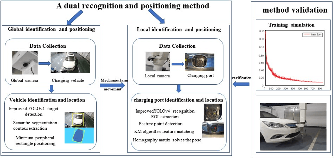
Electric vehicle charging identification and positioning is critically important to achieving automatic charging. In terms of the problem of automatic charging for electric vehicles, a dual recognition and positioning method based on deep learning is proposed. The method is divided into two parts: global recognition and localization and local recognition and localization. In the specific implementation process, the collected pictures of electric vehicle charging attitude are classified and labeled. It is trained with the improved YOLOv4 network model and the corresponding detection model is obtained. The contour of the electric vehicle is extracted by the BiSeNet semantic segmentation algorithm. The minimum external rectangle is used for positioning of the electric vehicle. Based on the location relationship between the charging port and the electric vehicle, the rough location information of the charging port is obtained. The automatic charging equipment moves to the vicinity of the charging port, and the camera near the charging gun collects pictures of the charging port. The model is detected by the Hough circle, the KM algorithm is used for feature matching, and the homography matrix is used to solve the attitude. The results show that the dual identification and location method based on the improved YOLOv4 algorithm proposed in this paper can accurately locate the charging port. The accuracy of the charging connection can reach 80%. It provides an effective way to solve the problems of automatic charging identification and positioning of electric vehicles and has strong engineering practical value.Graphic Abstract
Keywords
Highlights
The automatic charging of electric vehicles lacks a scheme suitable for large space identification and positioning. A dual identification and positioning scheme for multi vehicle automatic charging is determined.
Improve YOLOv4 algorithm to improve charging port detection speed.
Computer vision is most widely used in target detection. It mainly applies to target identification, localization, tracking, grasping, and other operations in robotic arm application research. It detects the object from the image with the help of optical sensors, key feature extraction by either hand-crafted feature detectors or learning-based models, and post-processing for the extracted features.
Traditional target detection algorithms are often used in face recognition, pedestrian detection and object detection. Traditional target detection algorithms include Haar-like feature extraction, Histograms of Oriented Gradients (HOG), Support Vector Machine (SVM), Deformable Parts Model (DPM), etc. Traditional detection algorithms for computer vision recognition are usually divided into three parts: (i) region selection, (ii) feature extraction and (iii) feature classification. Traditional detection algorithms typically use feature transformation for feature extraction, which results in limited extraction quality. The electric vehicle charging port is arranged differently in different brands, and the parking angle and direction of the electric vehicle to be charged are also different, resulting in the complexity and variability of the detection object. Traditional target detection algorithms cannot achieve effective detection, but deep learning can achieve the detection and extraction of complex targets.
With the rapid development of deep learning, researchers have started to use deep learning to achieve target detection. There are two types of target detection models based on deep learning, the one-step detection algorithm and the two-step detection algorithm. The two-step detection algorithm divides the detection problem into two stages. The first step is to generate candidate regions, then classify the candidate regions, and use the non-maximum suppression method to determine the target detection results [1]. Typical examples of such algorithms are R-CNN system algorithms based on candidate frames, such as R-CNN [2], Fast R-CNN [3], and Faster R-CNN [4], etc. Currently, the target detection task based on the image sensor is mainly completed by CNN. CNN has different detection effects on different targets in different scenes. Krizhevsky proposed AlexNet [5] to reduce the error rate of classification tasks. ResNet divides the network structure and connects the input and output directly through the shortcut structure [6], which effectively solves the problem of gradient disappearance. The R-CNN network proposed by Ren et al. [4] achieves end-to-end real-time deep learning target detection. Murugan et al. [7,8] improved the structure of R-CNN to achieve real-time target detection. Reference [9] combined Fast R-CNN with selective search to solve the problem of target loss in target detection. Qu et al. [10] began to use CNN to observe vehicle driving conditions and apply CNN for intelligent driving.
The one-step detection algorithm directly generates the category, probability and location coordinate value of the object. The typical algorithms include YOLO and SSD [11]. The one-step detection algorithm has the characteristics of low accuracy, high speed, poor detection effect of small objects, and high missed detection. The two-step algorithm has the characteristics of high precision, slow speed, and long training time. Currently, the most widely used algorithm is the YOLO series. YOLOv1 [12] performs well in speed, but it has poor group detection and weak generalization ability for small and close objects. Lin et al. proposed FPN [13] (feature pyramid network), which can be combined with the one-stage detection algorithm to improve the network processing ability of small targets. YOLOv2 [14] has improved detection accuracy and speed compared to YOLOv1, but the improvement in detection accuracy is not obvious because the underlying network of YOLOv2 is relatively simple. The underlying classification network darknet-53 of YOLOv3 [15] has a better performance. It also balances detection accuracy and detection speed for detection targets. YOLOv4 [16] and YOLOv5 [17] have made large-scale improvements based on YOLOv3. Both adopt the idea of CSPNet [18,19]. YOLOv4 adopts more data enhancement methods, the model is more holistic during training, while YOLOv5 uses a smaller network, which is very fast to train, but slightly less accurate than YOLOv4. Among the YOLO series algorithms, the network models of YOLOv3 and YOLOv4 algorithms are relatively complex, with significant computational cost and slow detection speed. Researchers propose some lightweight object detection algorithms for the above algorithms, such as YOLOv3-Tiny [20],YOLOv4-Tiny [21], MobileNetV1 [22], MobileNetV2 [23], MobileNetV3 [24] and others [25–30]. However, due to the simplification of the network model, the recognition accuracy is reduced, which cannot be applied to complex scenes and small target projects. The accuracy of target detection and positioning are vital for achieving the reliable connection between the charging gun and the charging port on the vehicle. YOLOv4 is more suitable for detecting electric vehicles and their charging ports because of its strong integrity and high detection accuracy. The owner of electric vehicle demands high efficiency and speed for automatic charging. The scenario of the electric vehicle charging is fixed, and the detection target information is complex. Therefore, to improve the detection speed while ensuring the accuracy of detection, it is necessary to improve the convolution neural network structure. It is of great significance to improve the network structure based on the detection algorithm of YOLOv4.
The remainder of this paper is organized as follows. Section 2 presents the overall identification and positioning scheme of electric vehicles. Section 3 introduces the identification and positioning methods of electric vehicles, and Section 4 introduces the identification and positioning methods of charging ports. Section 5 introduces the simulation results of charging recognition training and the docking experiment of electric vehicle automatic charging to verify the effectiveness of the overall scheme of electric vehicle automatic charging. We finalize the paper with some concluding remarks in Section 6.
2 Electric Vehicle Charging Identification and Positioning Scheme
The key to the research of automatic charging device is the recognition and positioning based on computer vision, and the recognition and positioning scheme depends on the location of electric vehicles, the mechanical configuration of the automatic charging device, the installation location and other factors [31]. The mechanical configuration design of the automatic charging device in this paper can accommodate different parking positions and attitudes of electric vehicles, but requires higher accuracy of the identification and positioning scheme. Therefore, this paper proposes a dual recognition and positioning scheme based on deep learning. As shown in Fig. 1, electric vehicle charging identification and positioning is divided into two processes: (i) global identification and positioning. (ii) local identification and positioning. The global identification and positioning process is as follows: when the electric vehicle is ready for charging, the global camera located in the control box starts to collect the vehicle pictures, identify and detect the vehicle through the YOLOv4 algorithm, extract the vehicle contour through semantic segmentation, locate the minimum external rectangle, obtain the spatial position coordinates of the vehicle, and convert the spatial position coordinates of the charging port in combination with the relative position information between the vehicle charging port and the coordinate system of the vehicle. The position information of the charging port obtained is rough. The local identification and positioning process is as follows: under the guidance of rough position information, the charging manipulator drives the charging gun to the area near the charging port, and the local camera starts to work. The local camera is used to collect the image of the charging port, and the precise space coordinates of the charging port are obtained by solving the Hough circle algorithm, KM algorithm and homography matrix, which is the accurate position of the charging port. Finally, this coordinate information guides the manipulator to complete the docking operation with the charging port.
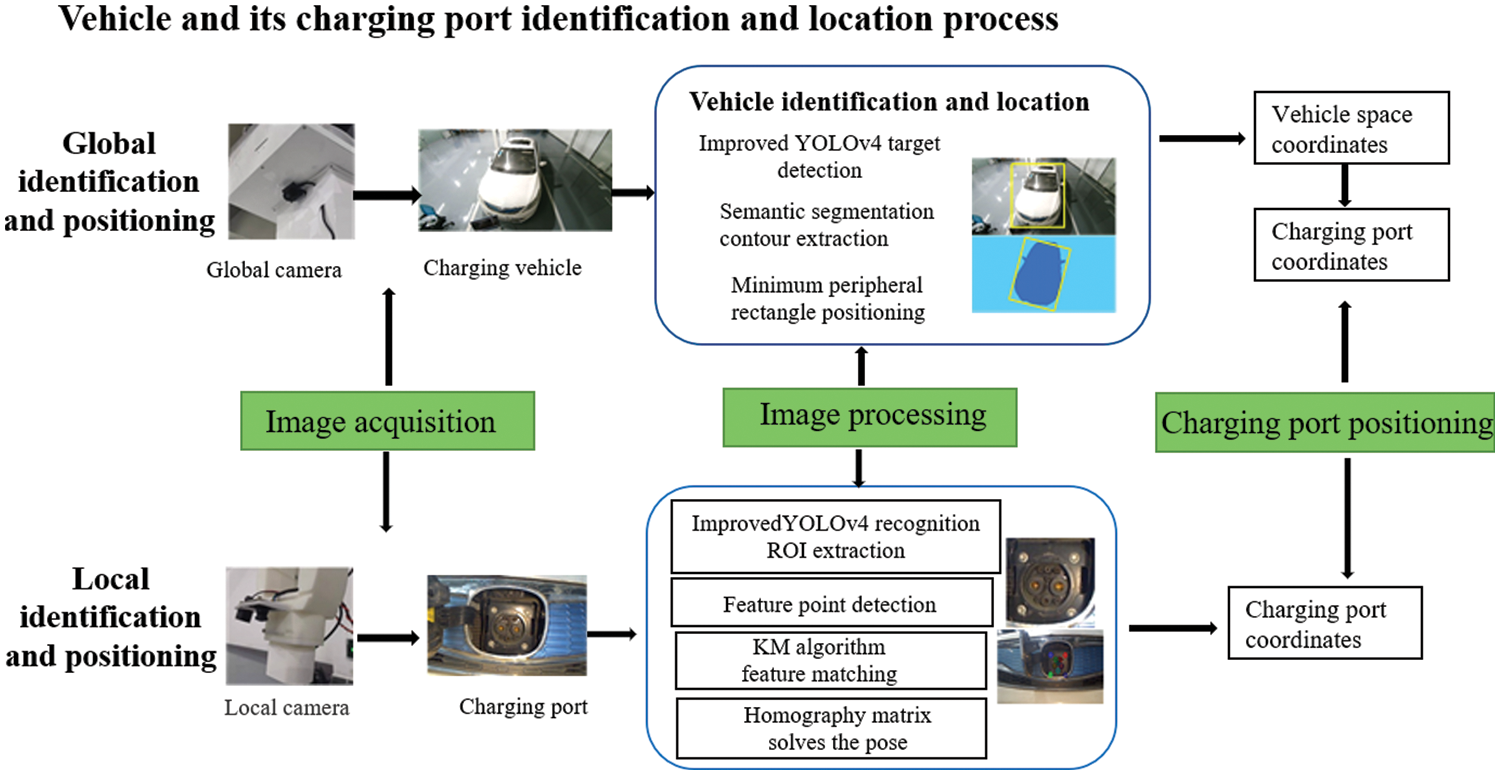
Figure 1: Electric vehicle charging identification and positioning scheme
3 Electric Vehicle Charging Identification and Positioning
The data processing pipeline is the prerequisite of visual positioning using deep learning. Pictures of the same vehicle with different head orientations and angles are collected as datasets. Car pictures taken should contain a complete outline. The processing of the dataset for training the model includes data collection, data annotation, dataset partition and dataset conversion.
The experimental vehicle is parked in the parking space, and the parking pictures of the vehicle in the front end and rear end are collected through the global camera. By controlling the robot arm to move randomly in the rectangular area composed of X-axis: 0–300 mm, Y-axis: 0–2500 mm, the vehicle can be located in different directions of the global camera imaging plane, and then different parking attitudes of the vehicle can be simulated. When the front of the vehicle is facing forward and the rear is facing forward, about 1000 parking images will be collected respectively, and a dataset with 2050 images will finally be formed as shown in Fig. 2.
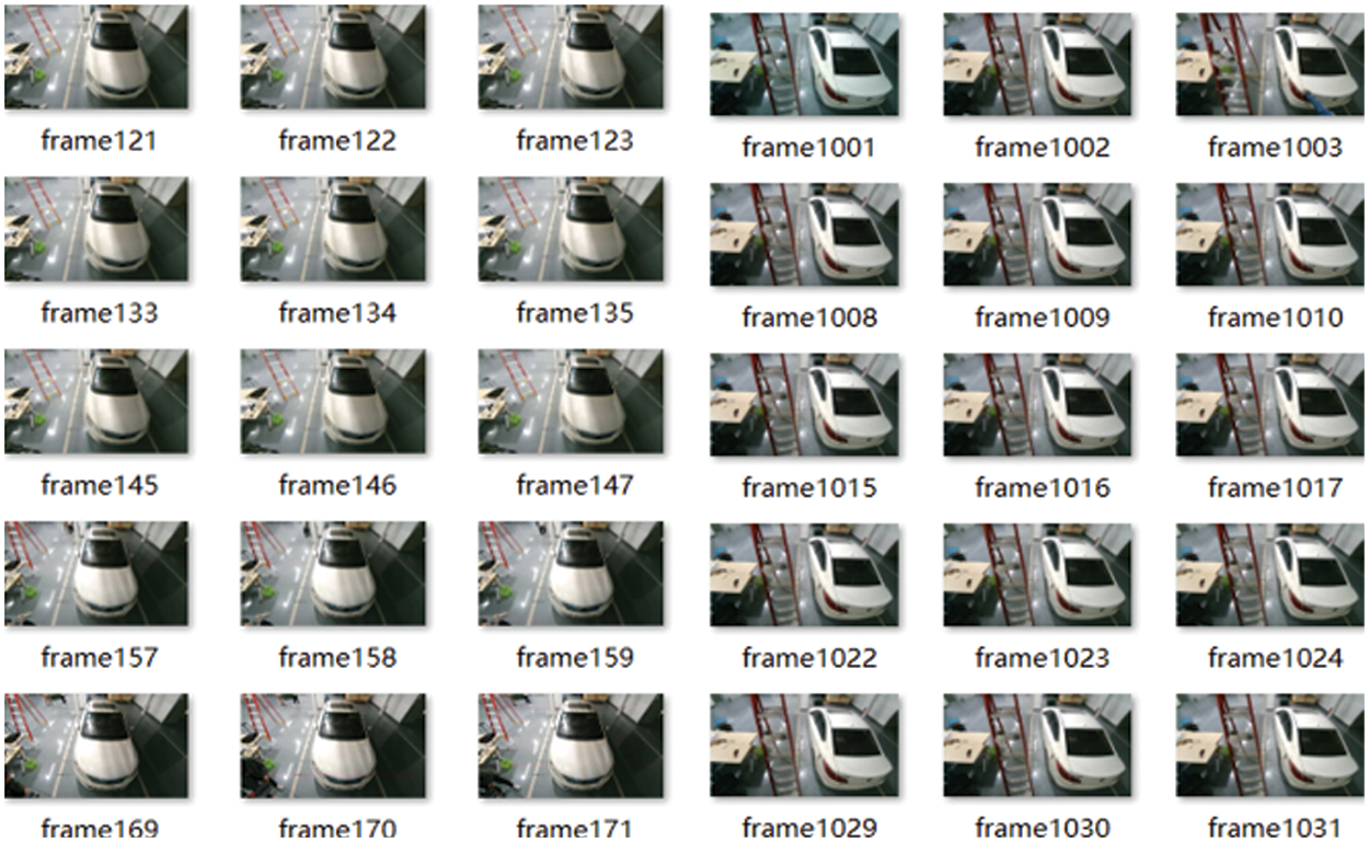
Figure 2: Dataset of vehicle parking images
Data annotation is the process of classifying, sorting, editing, correcting, marking and annotating collected images, and producing machine-readable data encoding that meets the requirements of machine learning and training. The vehicles in the images are labeled by bounding boxes to classify and distinguish them from the background and other objects. There are two kinds of labels involved, namely the front and the rear.
When training the deep learning model, the dataset will be divided into the training and the test sets. Due to the need to test the model and judge whether the training degree is overfitting or underfitting, the training data will be divided into two parts. One part is the training set and the other part is the verification set for testing. Verification sets can be reused, mainly to help build models. The training set is used to train the neural network model, and then the verification set is used to verify the effectiveness of the model to select the best model. Finally, after the model passes the verification set, we use the test set to evaluate the final performance, accuracy and error of the model.
In the current deep learning model training, after extensive research, the ratio between the training verification set and the test set is usually set to 9:1, in which the ratio between the training set and the verification set is set to 7:2 for optimal training results. In the YOLOv4 model training, the common practice was to set the ratio among the training set, the verification set, and the test set to 7:2:1. The entire dataset was divided automatically and randomly by the algorithm to obtain the partition results of training verification set and test set.
The annotated file contains various types of information, such as the name and the size of the picture, the category name and the location of the bounding box, etc. Necessary data conversion is required to pass proper parameters into the deep network during training.
3.2 Improved YOLOv4 Target Detection Algorithm
YOLOv4 is designed for real-time object detection and can run on low-end CPUs. The improved YOLOv4 is an enhanced variant of YOLOv4. Compared with YOLOv3, YOLOv4 has a variety of modifications on the backbone network based on the latter to achieve a perfect balance between running speed and detection accuracy. Fig. 3 shows the network structure of improved YOLOv4, which has more CSP structure and PAN structure than YOLOv3.
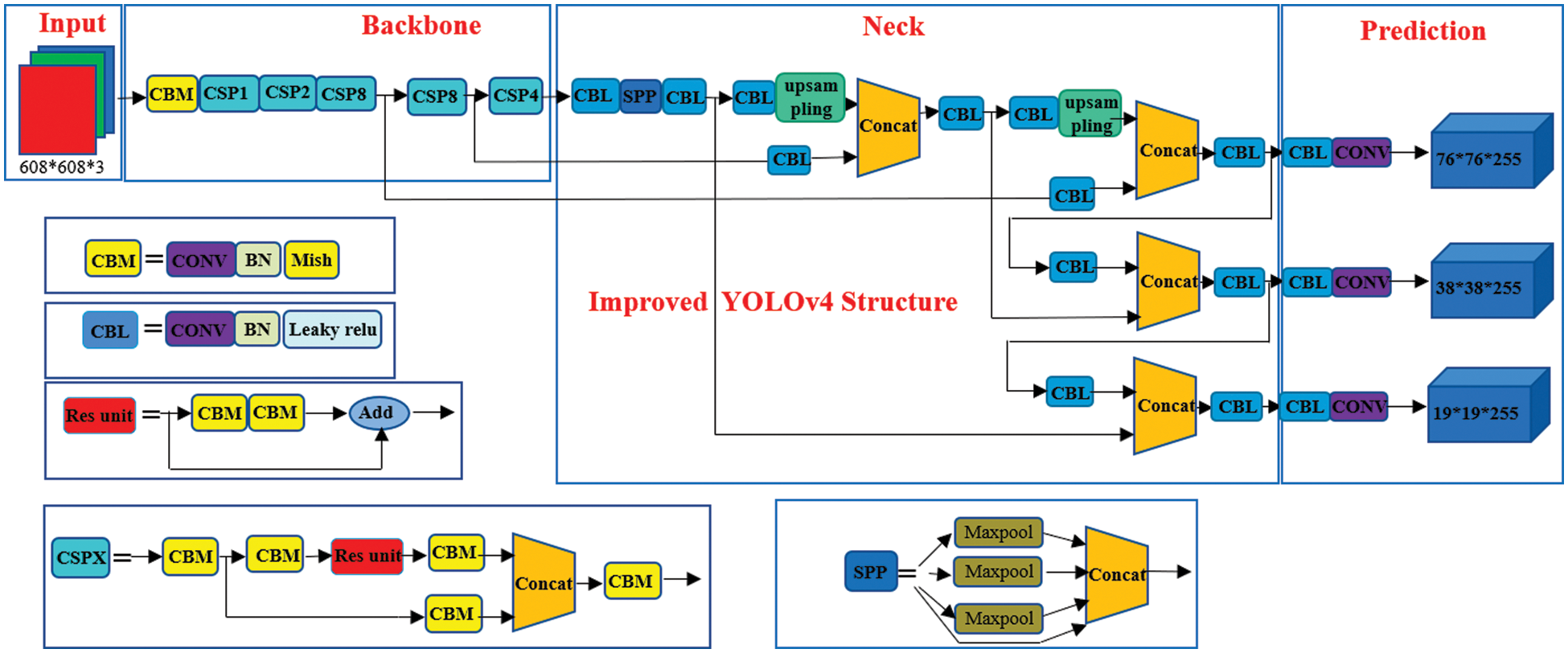
Figure 3: Improved YOLOv4 network structure diagram
In the design of CSPDarknet53, the calculation amount of CSPDarknet stage is whb2 (9/4 + 3/4 + 5k/2). From the formula, it can be seen that only when k > 1, CSPDarknet stage will have better computational advantages than the Darknet stage. The number of remaining layers in each stage of CSPDarknet53 is 1-2-8-8-4, respectively. In order to achieve a better balance between speed and accuracy, we convert the first CSP stage to the remaining layer of the original dark net. The calculation list of PAN architecture is shown in Fig. 4a. It mainly integrates features from different feature pyramids, and then passes through two groups of reverse dark net residual layers, with no shortcut connection. After CSP, the architecture of the new calculation list is shown in Fig. 4b. This new update effectively reduces the amount of computation by 40%.
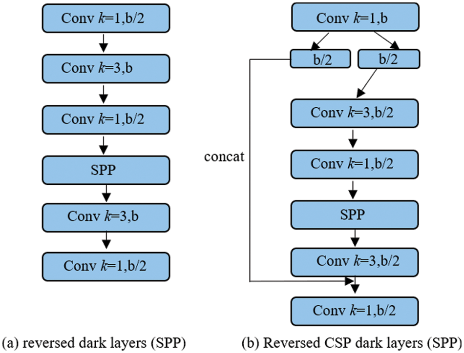
Figure 4: Computaional blocks of reversed dark layer (SPP) and reversed CSP dark layers (SPP)
Table 1 is the performance comparison between YOLOv3, YOLOv4 and improved YOLOv4 target detection algorithms. It indicates that after YOLOv4 is improved based on YOLOv3, AP can reach 48. The speed of the improved YOLOv4 is improved on the premise that the AP value of the training and test sets remains unchanged.

The input image is shown in Fig. 5a. The input image is processed by the original YOLOv4 model, and the result of inference is shown in Fig. 5b. The original images are trained by the self-trained YOLOv4 model, and the detection results are shown in Figs. 5c and 5d. The former is the detection result of the front-facing, and the latter is the detection result of the rear-facing.
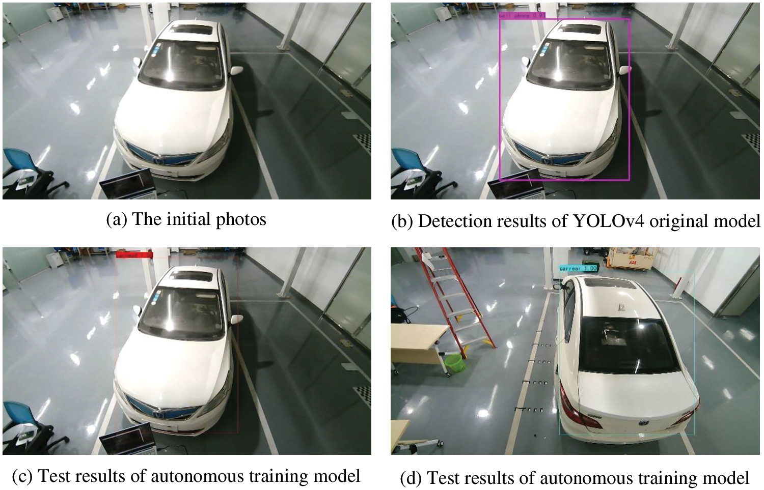
Figure 5: Detection results of YOLOv4 and autonomous training model
For the same picture, the original YOLOv4 model assigns multiple types to the detected object. Due to the complexity of the picture background, the recognition results of some objects are inaccurate, especially for detecting the target vehicle we are concerned about. However, after the YOLOv4 model is trained through the self-collected dataset, the test results will only identify the vehicles, and distinguish the front or rear categories.
3.3 Contour Extraction Based on BiSeNet Semantic Segmentation Algorithm
3.3.1 Segmentation Network BiSeNet
BiSeNet is a learning-based lightweight real-time semantic segmentation algorithm. Fig. 6 shows the network structure of BiSeNet. In general, the design idea of the whole network is to retain the spatial position information of objects and generate high-resolution feature maps through the design of small step spatial path (SP), as shown in Fig. 6a; The objective receptive field is obtained through the fast down sampling rate of the semantic path/context path (CP), as shown in Fig. 6b; Finally, a new feature fusion module (FFM) is added between SP and CP to fuse their feature maps, as shown in Fig. 6c, to achieve the balance between segmentation speed and accuracy.
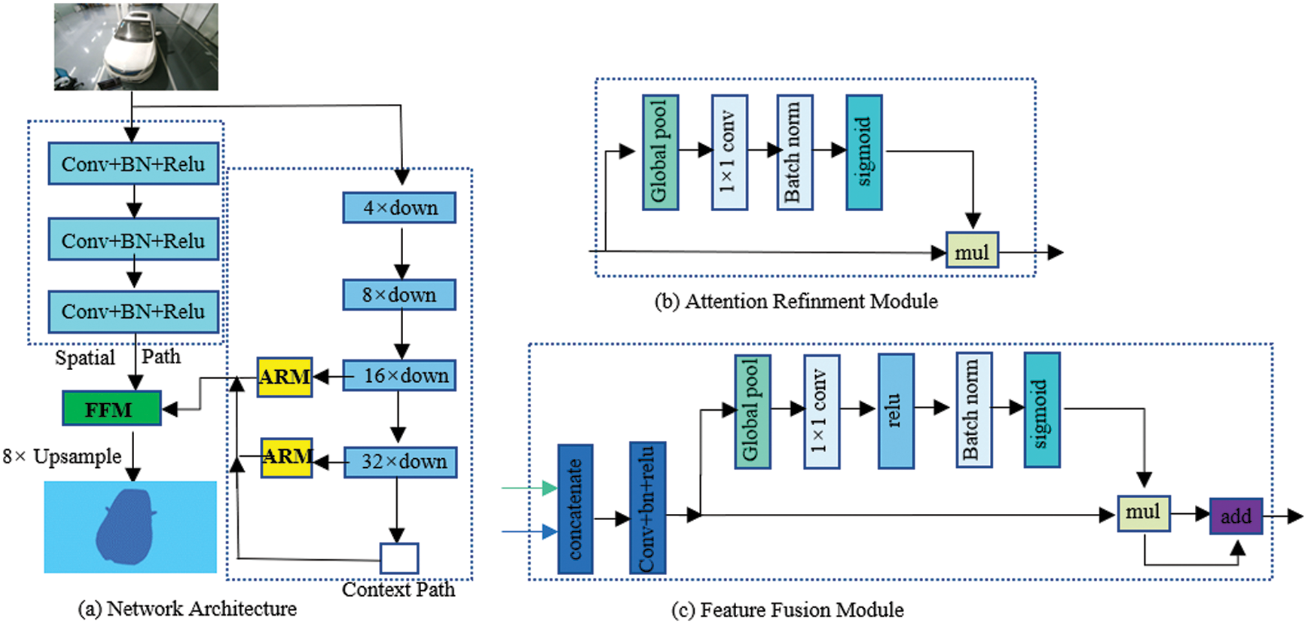
Figure 6: BiSeNet network structure diagram of bidirectional segmentation network
The experimental test shows that at the speed of 105 fps, the BiSeNet network has achieved 68.4% mIoU on the cityscapes test set, and achieved the design goal of simultaneously improving the speed and accuracy of real-time semantic segmentation. In addition, the lightweight network of BiSeNet is very suitable for use in the case of limited hardware memory and computational power. Therefore, this study finally decided to use BiSeNet network, combined with its own dataset, to train the real-time semantic segmentation model suitable for the proposed research scenario in this paper.
3.3.2 Dataset Annotation and Model Extraction
In order to extract the target contour, it is necessary to annotate the dataset. Combine the outline strokes of the scene information extracted from the dataset into a closed graph. Fig. 7 shows the data annotation of the picture when the head of the car facing position is different positions.
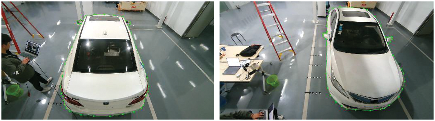
Figure 7: Vehicle semantic segmentation and extraction annotation
The weight file obtained after training is used for detection. The picture on the left of Fig. 8 is the initial input picture, and the middle and right of Fig. 8 are the segmentation results of BiSeNet model after autonomous training. For the same picture, the segmentation results of the original BiSeNet model have multiple object types, and due to the complexity of the picture background, the segmentation results of some objects are not very accurate. The whole segmentation results are chaotic, especially for the detection and segmentation of the target vehicle we are concerned about. After the BiSeNet model is trained through the self-collected dataset, the detection results will only segment the vehicle and the background.
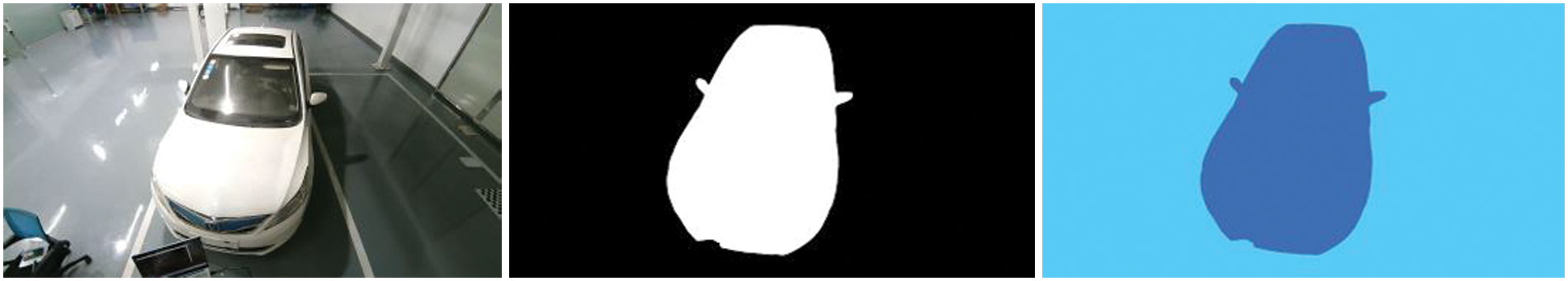
Figure 8: Training results of vehicle semantic segmentation
3.4 Minimum Circumscribed Rectangle Positioning
The minimum circumscribed rectangle refers to the maximum range of several two-dimensional shapes expressed in two-dimensional coordinates. The minimum rectangular boundary is determined by the maximum abscissa, minimum abscissa, maximum ordinate and minimum ordinate of each vertex of a given two-dimensional shape.
3.5 Main Steps of Minimum Circumscribed Rectangle Positioning
The shape of the vehicle to be charged is regular, which is a typical long strip, and the width and height of the smallest external rectangle are easy to extract. Therefore, the coordinates of the center point of the vehicle head and the deflection angle when the vehicle stops can be accurately obtained through this method. Suppose a point on the plane rotates by a certain angle around a fixed point, and suppose that a point (x1, y1) on the plane rotates counterclockwise around another point (x0, y0), and the rotation angle is θ. If the following point is (x2, y2), defined as
The coordinates of the center point (x′, y′) of the head (pixel coordinates) can be approximated by calculating the midpoint coordinates of the connecting line from the coordinates of the two vertices. By fusing the minimum circumscribed rectangle into the original image, the positioning accuracy can be roughly verified, as shown in Fig. 9. The result indicates that the positioning center point almost coincides with the center point of the vehicle head. The method of positioning with the minimum circumscribed rectangle is feasible. Then, according to the global camera calibration conversion relationship, the coordinates (x, y) of the head center point in the world space coordinate system are obtained.
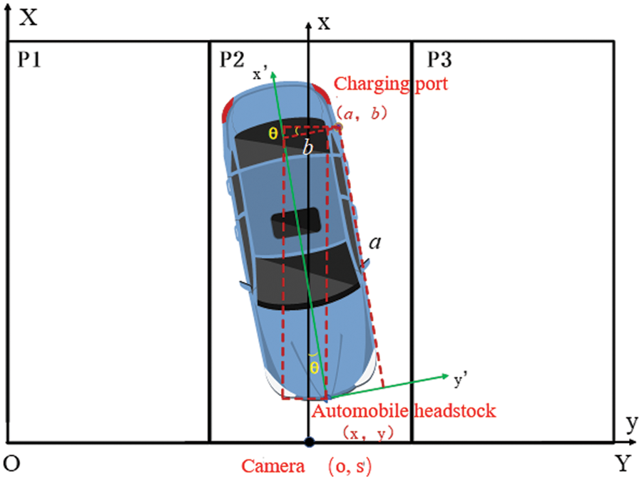
Figure 9: Relative coordinate conversion relation
In the camera recognition and positioning process, four coordinate systems, including world coordinate system, camera coordinate system, image coordinate system and pixel coordinate system, are involved. The transformation relationship between them is shown below:
The four coordinate systems are defined as follows:
(Xw, Yw, Zw): World coordinate system, which describes the position of the camera, and the unit is m.
(Xc, Yc, Zc): Camera coordinate system, optical center as origin, and the unit is m.
(x, y): Image coordinate system. The optical center is the image center. The origin o is located at the intersection of the optical axis and the projection plane. Its coordinates under the pixel coordinate system are (u0, v0). The x-axis and y-axis are parallel to the projection plane, and the unit is mm.
(u, v): Pixel coordinate system, the origin is the upper left corner of the image, and the u and v axis coincides with both sides of the projection plane. This coordinate system is in the same plane as the image coordinate system, but the origin is at the upper left corner of the image, and the unit is pixel.
P: A point in the world coordinate system, that is, a point in the real world.
p: For the imaging point of point P in the image, the coordinates in the image coordinate system are (x, y) and the coordinates in the pixel coordinate system are (u, v).
f: Camera focal length, equal to O and OC distance.
The internal parameter K =
4 Charging Port Identification and Positioning
The charging port identification and positioning require local positioning, and the sensor used in this process is a local camera. Firstly, the calibrated camera is used to collect the image of the vehicle charging port, and the image processing operations, such as YOLOv4 recognition and ROI extraction, feature point Hoff circle detection, KM algorithm feature matching, homography matrix solving attitude, are performed on the image. Finally, we can obtain the location information of the vehicle charging port, and complete the docking between the charging gun and the charging port.
4.1 Charging Port Image Collection
In the process of global identification and positioning, the general position information of the charging port is obtained. The position information guides the mechanical arm joint to drive the charging gun to move to the area near the charging port. The local camera starts to work to collect the image information of the area near the charging port, as shown in Fig. 10.
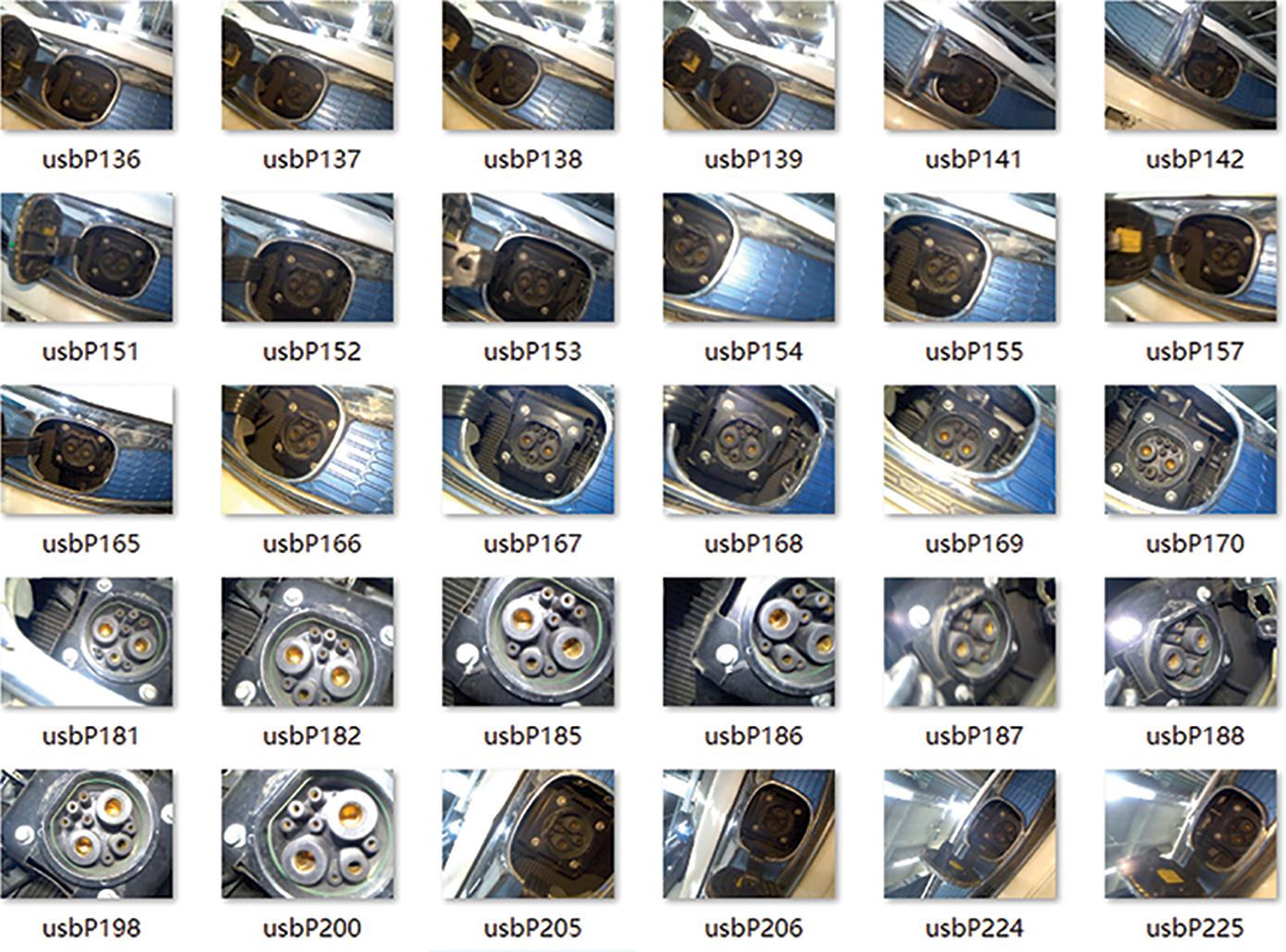
Figure 10: Charging port dataset
4.2 ROI Extraction of Charging Port Based on YOLOv4 Recognition
After the charging port image is collected, the image needs to be preprocessed. First, the preprocessing determines whether there is a complete charging port in the picture or not. If there is no charging port or only part of the charging port, the local camera position is adjusted to recollect the charging port image. Suppose there is a charging port in the collected picture. In that case, the position of the charging port in the picture is extracted, and the charging port area is segmented to remove the interference of the background part.
YOLOv4 is used to draw a bounding box to locate the charging port when identifying the charging port, as shown in Fig. 11. The position and size information of the rectangular box is used to segment the original picture and extract the charging port area. ROI extraction is adopted for charging port extraction, which can reduce image processing time and increase recognition accuracy, as shown in Fig. 12.
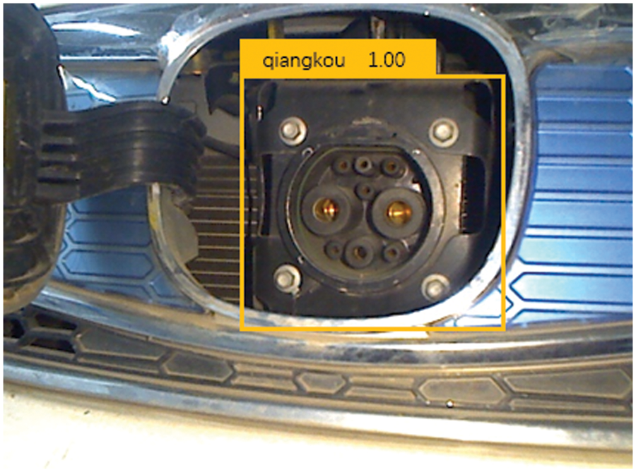
Figure 11: YOLOv4 identification charging port
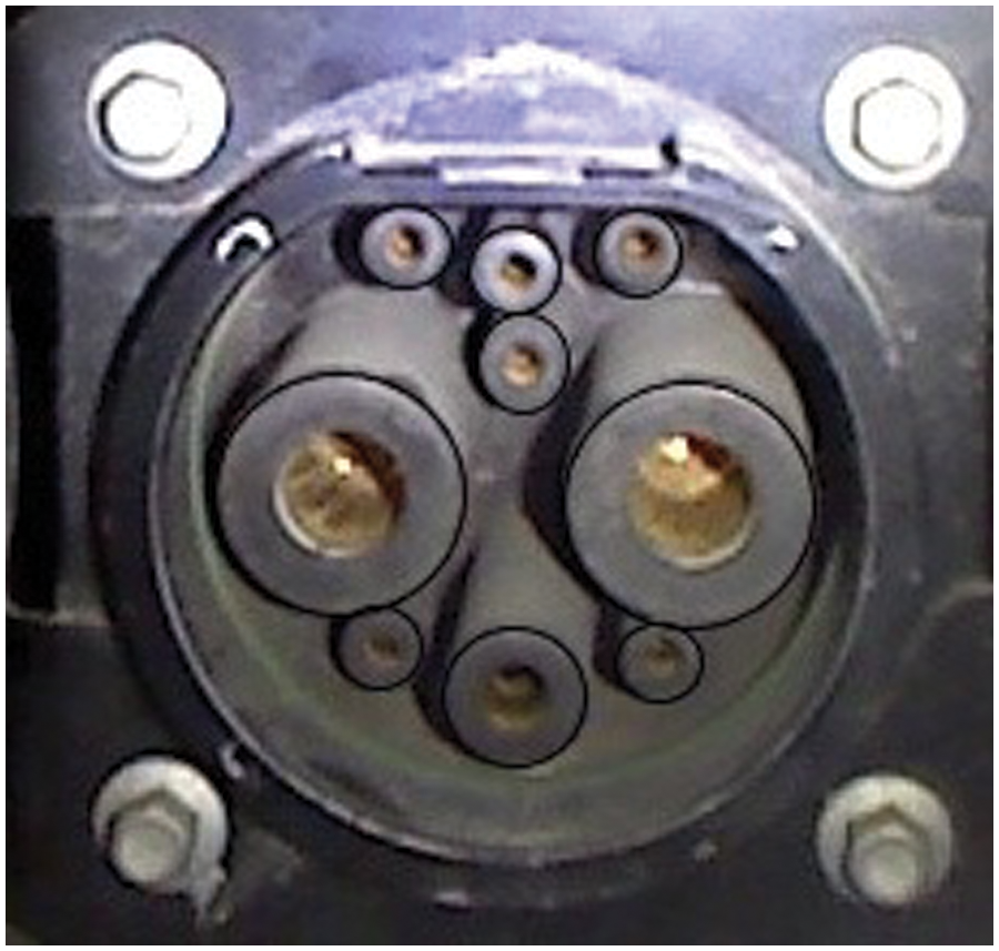
Figure 12: ROI extraction charging port area
4.3 Feature Point Detection Based on Hough Circle Transform
The purpose of feature point detection is to obtain the obvious feature points of the charging port in the picture to be detected for matching and locating. As the quick charging port of the vehicle is an industry standard with fixed size and shape, the feature points of the charging port are extracted through Hough transform circle detection.
The Hough transform algorithm is used to detect the Hough circle of the target picture and the position picture, as shown in Fig. 13. Then, by taking the center of each circle as the feature point, the center coordinate value is recorded, and a series of feature points is outputted. In this way, the feature points of the two pictures are detected and extracted for subsequent matching.
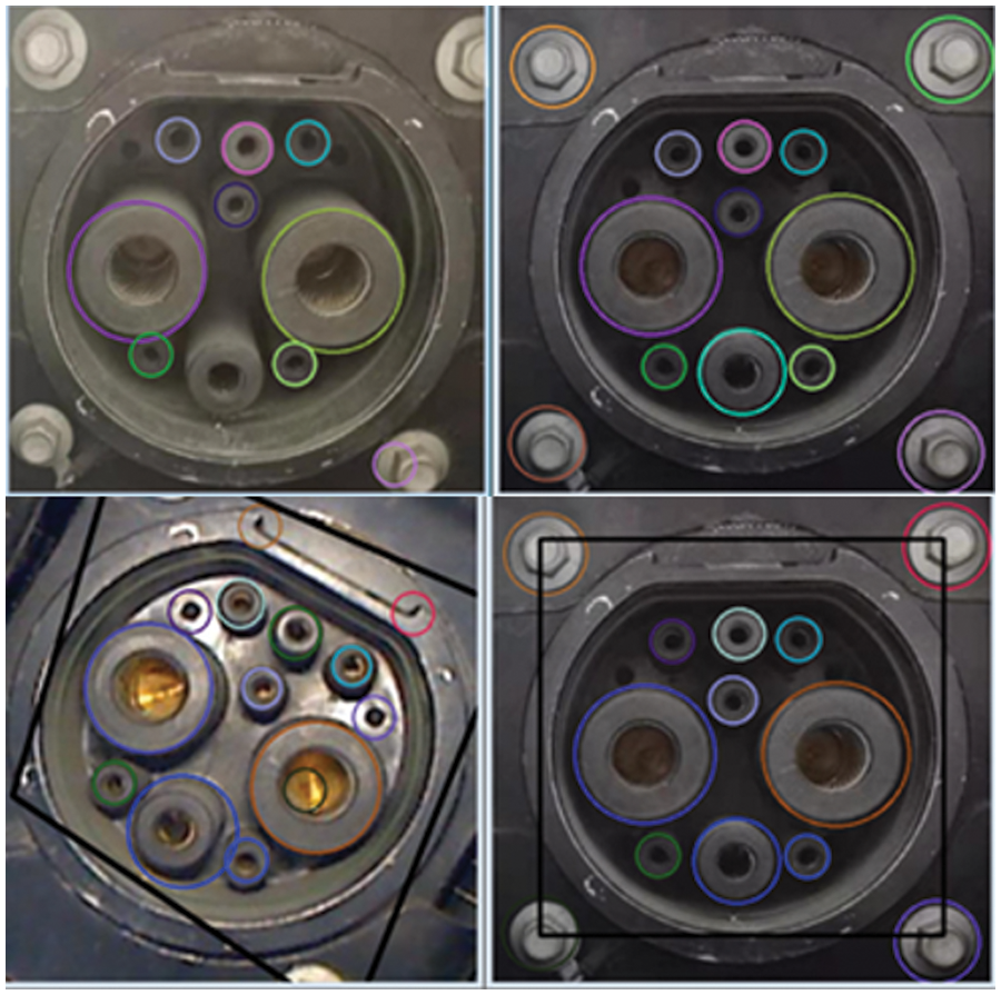
Figure 13: Hough transform circle detection and feature point extraction
4.4 KM Algorithm Feature Matching
The information matching degree of the image to be detected and the positioning reference image is related to the acquisition position. The closer the position is, the higher the matching degree is. The reciprocal of distance is used as the weight of KM algorithm, and the weight calculation formula is shown in formula (7).
where k is a fixed parameter, dis represents distance calculation, and P = (a, b, r) is the center coordinate and radius of the circle represented by each feature point.
4.5 Homography Matrix for Solving Camera Position
There is homography between images of the same plane object taken from different positions by a camera without lens distortion, which can be expressed by projection transformation. This projection transformation matrix is called homography matrix.
As shown in Fig. 14, there is an object in space. Two pictures are taken with the camera at different angles, and both pictures have P points. The pixel coordinates of P points in the two pictures are P1 (u1, v1) and P2 (u2, v2). The transformation relationship between these two coordinates is homography transformation, P1 = HP2.
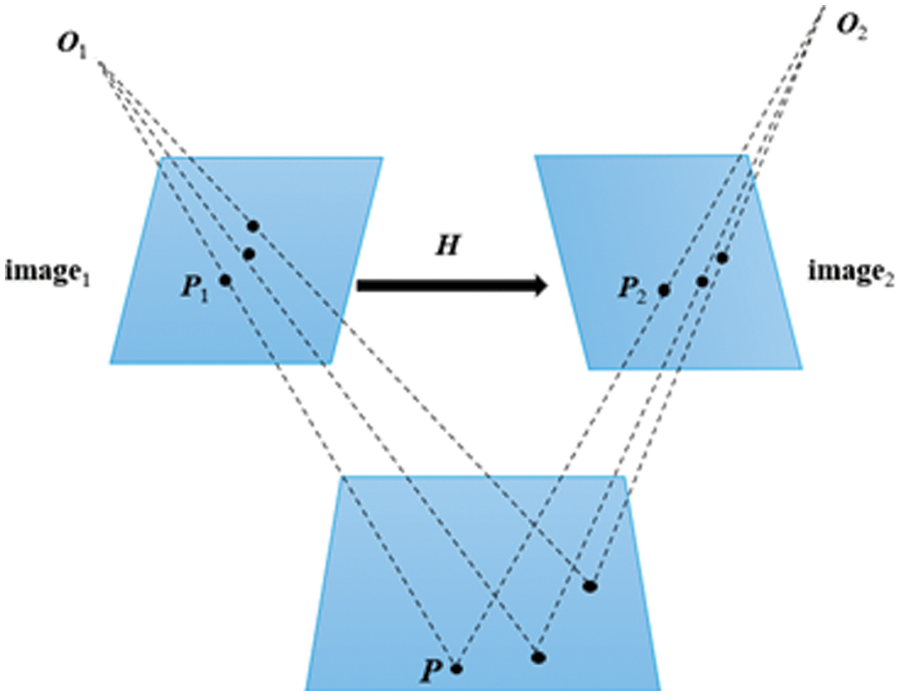
Figure 14: Homography matrix transformation relationship
Decomposition formula (6) can be given:
where
P = [X Y Z]T is a point in space. The image taken by the camera in its initial position is image1, it is the positioning reference picture. At this time, the motion of the camera has no rotation and translation. R is the identity matrix, T is 0. P is a point in the image, the pixel coordinates of point P in image1 is P1 (u1, v1, 1), it meets:
After the camera moves through rotation and translation, take the picture image2, it is the picture to be detected. The picture contains the spatial point P, so the pixel coordinate of point P in image2 is P2 (u2, v2, 1), it meets:
Point P is on a plane in space, the definition of space plane is
According to formulas (9)–(11), we can get:
After simplification, we can get:
where s1 and s2 are scale factors, due to the scale invariance of P1 and P2, s1 and s2 do not consider specific values.
From the above formula, homography matrix H is related to the parameters of rotation, translation and plane. In homogeneous coordinates, the H is also a 3 * 3 matrix. The solution idea is to calculate according to the matching points, and then decompose it to calculate the camera external parameter rotation matrix and translation matrix.
Expand formula (8), we can get:
Normalize H, multiply by a non-zero factor to meet h9 = 1, H has 8 degrees of freedom and 8 unknown variables. Expand formula (15), we have:
After simplification, we can get:
A set of matching point pairs P1 and P2 can construct two constraints, so the homography matrix with a degree of freedom of 8 can be calculated through four sets of non-collinear matching point pairs.
5 Charging Port Identification Simulation and Charging Connection Experiment
The identification and positioning of the charging port are first trained by the charging port data set, and the training effect of the charging port data set is related to training samples. We need to save the loss value generated in the training process, draw the loss map, and simulate the charging port recognition training process. As shown in Fig. 15, 800 training iterations resulted in 800 loss values. At the beginning of the training, the loss value is 0.15. As the iteration process progresses, when the number of iterations is 600, the loss value converges to 0.1. The training effect is good.
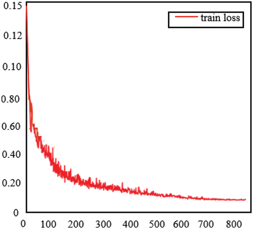
Figure 15: Loss of charging port identification training
The automatic charging device obtains the position of the global charging port through global identification and positioning, and the mechanical arm drives the charging gun to move near the position of the charging port. The local camera starts to work, and after local identification and positioning, the accurate location of the charging port is obtained. During the identification process, multiple local positioning processes will be carried out to improve the accuracy of docking.
Fig. 16 shows the process of automatic charging docking experiment. Repeat the robot arm automatic charging docking experiment for 10 times to verify the effectiveness of identification and positioning based on deep learning. Record the completion result and time of automatic charging docking.
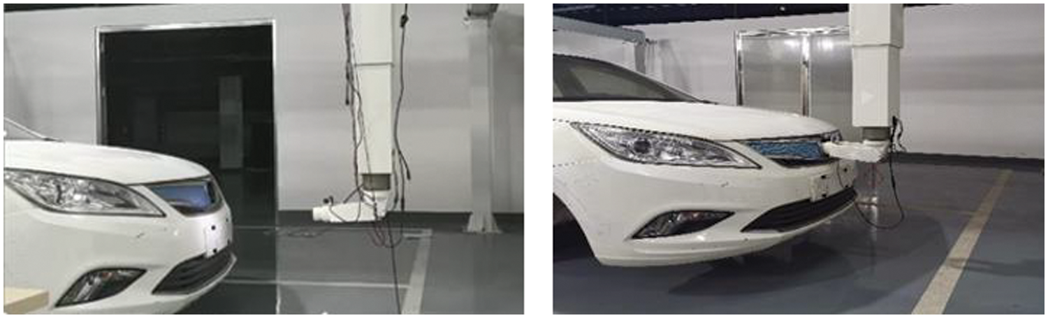
Figure 16: Experimental process of automatic charging and docking of manipulator
As shown in Table 2, 8 of the 10 experiments have successfully completed the docking of the charging gun and the charging port, with a success rate of 80%, which proves the effectiveness and practical significance of the dual identification and positioning method based on deep learning.

At present, the research on the automatic charging device of electric vehicles mostly focuses on the design scheme of the industrial robot clamping charging gun. The identification space of the charging port is only limited to the activity space of the mechanical arm, and the charging space is small. Therefore, the identification and positioning scheme of the charging port uses a single camera for identification and positioning, and the docking accuracy is low. In view of the above research status, this paper proposes a dual identification and location scheme for multi vehicle automatic charging. This scheme has a large recognition space and can be compatible with the recognition of charging ports of various vehicle models. The accuracy of the charging connection is high, up to about 80%. On the premise that the docking accuracy error does not exceed 5%, further improve the docking speed of automatic charging, propose an improved YOLOv4 network structure, and the convergence speed of the network structure has been significantly improved. Finally, 10 charging and docking experiments are conducted for the above research to verify the effectiveness of the dual identification and location scheme based on the improved YOLOv4 algorithm. This paper solves the problem of low identification and positioning accuracy in large space range of multi vehicle automatic charging, and also improves the charging connection speed. In future research, we should further improve the accuracy of target detection, consider the charging time while improving the accuracy, and improve the slow charging problem in the current automatic charging field.
Funding Statement: This work is supported by Guangdong Province Key Research and Development Project (2019B090909001), National Natural Science Foundation of China (52175236), the Natural Science Foundation of China (Grant 51705268) and China Postdoctoral Science Foundation Funded Project (Grant 2017M612191).
Conflicts of Interest: The authors declare that they have no conflicts of interest to report regarding the present study.
References
1. Neubeck, A., Gool, L. V. (2006). Efficient non-maximum suppression. International Conference on Pattern Recognition, pp. 850–855. Hong Kong, China. https://doi.org/10.1109/ICPR.2006.479 [Google Scholar] [CrossRef]
2. Girshick, R., Donahue, J., Darrell, T., Malik, J. (2014). Rich feature hierarchies for accurate object detection and semantic segmentation. 2014 IEEE Conference on Computer Vision and Pattern Recognition (CVPR), pp. 580–587. Columbus, OH. https://doi.org/10.1109/CVPR.2014.81 [Google Scholar] [CrossRef]
3. Girshick, R. (2015). Fast R-CNN. 2015 IEEE International Conference on Computer Vision (ICCV), pp. 1440–1448. Santiago, Chile. https://doi.org/10.1109/ICCV.2015.169 [Google Scholar] [CrossRef]
4. Ren, S., He, K., Girshick, R., Sun, J. (2015). Faster R-CNN: Towards real-time object detection with region proposal networks. Advances in Neural Information Processing Systems, 39(6), 1137–1149. https://doi.org/10.1109/TPAMI.2016.2577031 [Google Scholar] [PubMed] [CrossRef]
5. Krizhevsky, A., Sutskever, I., Hinton, G. E. (2012). Imagenet classification with deep convolutional neural networks. Communications of the ACM, 60(6), 84–90. https://doi.org/10.1145/3065386 [Google Scholar] [CrossRef]
6. He, K., Zhang, X., Ren, S., Sun, J. (2016). Deep residual learning for image recognition. 2016 IEEE Conference on Computer Vision and Pattern Recognition (CVPR), pp. 770–778. Las Vegas, NV, USA. https://doi.org/10.1109/CVPR.2016.90 [Google Scholar] [CrossRef]
7. Murugan, V., Vijaykumar, V., Nidhila, A. (2019). A deep learning R-CNN approach for vehicle recognition in traffic surveillance system. 2019 International Conference on Communication and Signal Processing (ICCSP), pp. 0157–0160. Chennai, India. https://doi.org/10.1109/ICCSP.2019.8698018 [Google Scholar] [CrossRef]
8. Liu, X., Liu, W., Mei, T., Ma, H. (2016). A deep learning-based approach to progressive vehicle re-identification for urban surveillance. 14th European Conference on Computer Vision (ECCV), vol. 9906, pp. 869–884. Amsterdam, Netherlands. https://doi.org/10.1007/978-3-319-46475-6_53 [Google Scholar] [CrossRef]
9. Shi, K., Bao, H., Ma, N. (2017). Forward vehicle detection based on incremental learning and fast R-CNN. 13th International Conference on Computational Intelligence and Security (CIS), pp. 73–76. Hong Kong, China. https://doi.org/10.1109/CIS.2017.00024 [Google Scholar] [CrossRef]
10. Qu, Y., Jiang, L., Guo, X. (2016). Moving vehicle detection with convolutional networks in UAV videos. 2nd International Conference on Control, Automation and Robotics (ICCAR), pp. 225–229. Hong Kong, China. https://doi.org/10.1109/ICCAR.2016.7486730 [Google Scholar] [CrossRef]
11. Liu, W., Anguelov, D., Erhan, D., Szegedy, C., Reed S. et al. (2016). SSD: Single shot multibox detector. 14th European Conference on Computer Vision (ECCV), pp. 21–37. Amsterdam, Netherlands. https://doi.org/10.1007/978-3-319-46448-0_2 [Google Scholar] [CrossRef]
12. Redmon, J., Divvala, S., Girshick, R., Farhadi, A. (2016). You only look once: Unified, real-time object detection. 2016 Conference on Computer Vision and Pattern Recognition (CVPR), pp. 779–788. Seattle, WA. https://doi.org/10.1109/CVPR.2016.91 [Google Scholar] [CrossRef]
13. Lin, T. Y., Dollár, P., Girshick, R., He, K., Hariharan, B. et al. (2016). Feature pyramid networks for object detection. arXiv:1612.03144. [Google Scholar]
14. Redmon, J., Farhadi, A. (2017). YOLO9000: Better, faster, stronger. 30th IEEE Conference on Computer Vision Pattern Recognition (CVPR), pp. 6517–6525. Honolulu, HI. https://doi.org/10.1109/CVPR.2017.690 [Google Scholar] [CrossRef]
15. Redmon, J., Farhadi, A. (2018). YOLOv3: An incremental improvement. arXiv:1804.02767v1. [Google Scholar]
16. Bochkovskiy, A., Wang, C. Y., Liao, H. (2020). YOLOv4: Optimal speed and accuracy of object detection. arXiv:2004.10934. [Google Scholar]
17. Wang, J., Chen, Y., Gao, M., Dong, Z. (2021). Improved YOLOv5 network for real-time multi-scale traffic sign detection. arXiv:2112.08782. [Google Scholar]
18. Liu, T., Zhou, B., Zhao, Y., Yan, S. (2021). Ship detection algorithm based on improved YOLO v5. 2021 6th International Conference on Automation, Control and Robotics Engineering (CACRE), pp. 483–487. Dalian, China. https://doi.org/10.1109/CACRE52464.2021.9501331 [Google Scholar] [CrossRef]
19. Wang, C. Y., Liao, H., Wu, Y. H., Chen, P. Y., Yeh, I. H. (2020). CSPNet: A new backbone that can enhance learning capability of CNN. IEEE/CVF Conference on Computer Vision and Pattern Recognition Workshops (CVPRW), pp. 1571–1580. https://doi.org/10.1109/CVPRW50498.2020.00203 [Google Scholar] [CrossRef]
20. Adarsh, P., Rathi, P., Kumar, M. (2020). YOLO V3-Tiny: Object detection and recognition using one stage improved model. 6th International Conference on Advanced Computing and Communication Systems (ICACCS), pp. 687–694. Coimbatore, India. https://doi.org/10.1109/ICACCS48705.2020.9074315 [Google Scholar] [CrossRef]
21. Wang, C. Y., Bochkovskiy, A., Liao, H. (2021). Scaled-YOLOv4: Scaling cross stage partial network. IEEE/CAF Conference on Computer Vision and Pattern Recognition (CVPR), pp. 13024–13033. https://doi.org/10.1109/CVPR46437.2021.01283 [Google Scholar] [CrossRef]
22. Howard, A. G., Zhu, M., Chen, B., Kalenichenko, D., Wang, W. et al. (2017). MobileNets: Efficient convolutional neural networks for mobile vision applications. arXiv:1704.04861. [Google Scholar]
23. Sandler, M., Howard, A., Zhu, M., Zhmoginov, A., Chen, L. C. (2018). MobileNetV2: Inverted residuals and linear bottlenecks. 31st IEEE/CVF Conference on Computer Vision and Pattern Recognition (CVPR), pp. 4510–4520. Salt Lake City, UT. https://doi.org/10.1109/CVPR.2018.00474 [Google Scholar] [CrossRef]
24. Howard, A., Sandler, M., Chu, G., Chen, L. C., Chen, B. et al. (2019). Searching for MobileNetV2. IEEE/CVF International Conference on Computer Vision (ICCV), pp. 1314–1324. Seoul, South Korea. https://doi.org/10.1109/ICCV.2019.00140 [Google Scholar] [CrossRef]
25. Zhang, X., Zhou, X., Lin, M., Sun, J. (2019). ShuffleNet: An extremely efficient convolutional neural network for mobile devices. 31st IEEE/CVF Conference on Computer Vision and Pattern Recognition (CVPR), pp. 6848–6856. Salt Lake City, UT. https://doi.org/10.1109/CVPR.2018.00716 [Google Scholar] [CrossRef]
26. Ma, N., Zhang, X., Zheng, H. T., Sun, J. (2018). ShuffleNet v2: Practical guidelines for efficient CNN architecture design. 15th European Conference on Computer Vision (ECCV), vol. 11218, pp. 116–131, Munich. https://doi.org/10.1007/978-3-030-01264-9_8 [Google Scholar] [CrossRef]
27. Xiong, Y., Liu, H., Gupta, S., Akin, B., Bender, G. et al. (2021). Mobiledets: Searching for object detection architectures for mobile accelerators. IEEE/CVF Conference on Computer Vision and Pattern Recognition (CVPR), pp. 3825–3834. https://doi.org/10.1109/CVPR46437.2021.00382 [Google Scholar] [CrossRef]
28. Huang, G., Liu, S., Van der Maaten, L., Weinberger, K. Q. (2018). CondenseNet: An efficient densenet using learned group convolutions. 31st IEEE/CVF Conference on Computer Vision and Pattern Recognition (CVPR), pp. 2752–2761. Salt Lake City, UT. https://doi.org/10.1109/CVPR.2018.00291 [Google Scholar] [CrossRef]
29. Wong, A., Famuori, M., Shafiee, M. J., Li, F., Chwyl, B. et al. (2019). Yolo Nano: A highly compact you only look once convolutional neural network for object detection. arXiv.1910.01271. [Google Scholar]
30. Qin, Z., Li, Z., Zhang, Z., Bao, Y., Yu, G. et al. (2019). ThunderNet: Towards real-time generic object detection on mobile devices. IEEE/CVF International Conference on Computer Vision (ICCV), pp. 6718–6727. Seoul, South Korea. https://doi.org/10.1109/ICCV.2019.00682 [Google Scholar] [CrossRef]
31. Carra, M., Maternini, G., Barabino, B. (2022). On sustainable positioning of electric vehicle charging stations in cities: An integrated approach for the selection of indicators. Sustainable Cities and Society. 85. https://doi.org/10.1016/j.scs.2022.104067 [Google Scholar] [CrossRef]
Cite This Article
 Copyright © 2023 The Author(s). Published by Tech Science Press.
This work is licensed under a Creative Commons Attribution 4.0 International License , which permits unrestricted use, distribution, and reproduction in any medium, provided the original work is properly cited.
 Downloads
 Citation Tools