Interactive Restoration of Three-Dimensional Implicit Surface with Irregular Parts

1  Introduction

Implicit representation is a common method for defining three-dimensional shapes and has advantages in many applications, such as shape modeling in computer graphics, physics-based simulation, material science, and medical imaging. One important application of implicit representation is shape modeling based on constructive solid geometry, skeletal modeling, and blending, among others [1,2]. Three-dimensional shapes can be effectively structured as combinations of primitives using algebraic operations. Another application of implicit representation is the shape modeling of obstacles for particle-based fluid simulation [3,4]. Implicit representation helps to efficiently estimate boundary force to fluid particles when the particles approach obstacles. It is also useful for shape modeling of complex materials, such as composite porous and molecular surfaces [5–7]. In these applications, such structures of complex materials and molecules are generated procedurally and defined as isosurfaces of scalar fields.

An implicit surface reconstruction from a set of surface points is a typical problem in computer graphics and several methods for the automatic generation of scalar fields have been proposed since the 1990s. Section 2 provides a brief review of the implicit surface reconstruction methods. However, as mentioned in several articles [8–12], the quality of reconstructed surfaces is sometimes poor depending on the density and accuracy of the given surface points. Defects, such as missing points, noise, and nonuniform sampling, often result in generated shapes with irregular components, such as redundant protrusions and noisy-liked jaggy components. Fig. 1 gives two examples of irregular implicit surfaces.

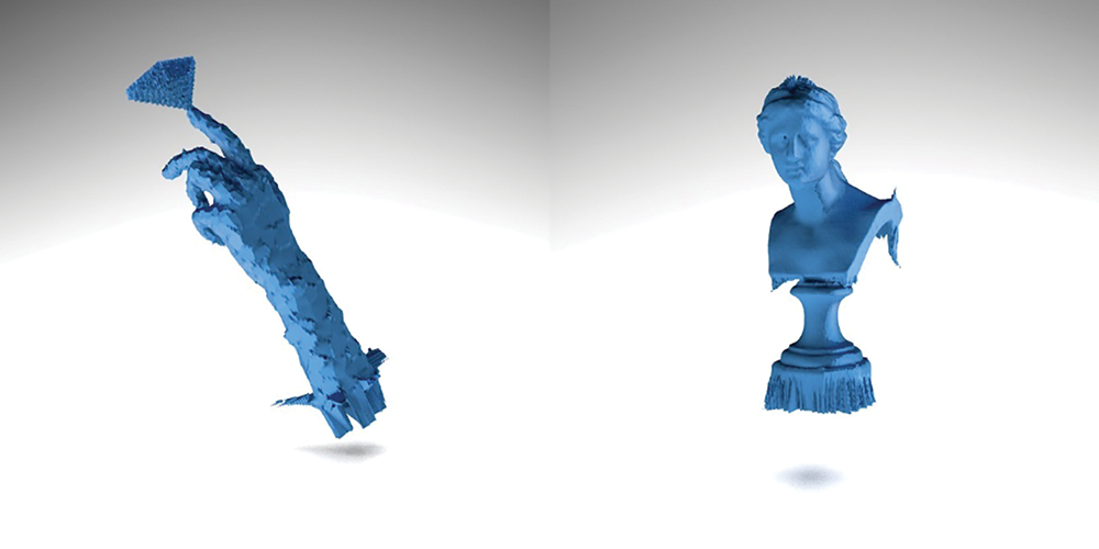
Figure 1: Examples of irregular surfaces generated based on piecewise polynomials [13,14]. Left: surface “Hand” with noisy and protruding components; the point data is provided by Rapidform (INUS Technology, Inc., USA). Right: surface “Venus” with protruding components; the point data is generated using a 3D scanning system

In this paper, we provide solutions for restoring irregular implicit surfaces. We focus on two major surface irregularities: redundant protrusions and jaggy noise. We assume that users specify masks in three-dimensional space and that restoration is performed only in the masked region. If a mask is specified to cover a redundant protrusion on a surface, our method updates the masked region by replacing the long protruding part with a round or flat-shaped surface. Users can control the roundness/flatness of the restored portion of the surface. The new scaler field within the mask is generated as the least-square solution of Laplace’s equation with both Dirichlet and Neumann conditions. The Dirichlet boundary condition is used to guarantee continuity at the border of the mask, while the Neumann boundary condition is used to control the roundness/flatness. Similarly, users can specify the region of restoration of jaggy noise by a mask that covers the region. Furthermore, users can control the degree of noise reduction by a parameter. Noise reduction is performed through low-resolution resampling within the mask. The final scaler field is generated by dense spline interpolation of the entire domain, with the spline ensuring continuity.

2  Related Work

Shape representation can be performed in various ways. Traditionally, shapes can be represented by enumerating small geometric elements and allowing them to cover the surface, a technique known as explicit representation [15,16]. The advantage of this approach is that the surface can be extended arbitrarily based on the users’ needs. Another prospective approach for representing a shape is to find an appropriate field defined by the function f(x), where x is a point in N-dimensional space, and the shape is considered the zero-value set of the field, when f(x)=0. This idea is known as implicit representation and it is feasible to generate shapes without having to enumerate elements over the shape. One approach for determining the field f(x) is an implicit surface reconstruction from a set of oriented surface points. Given a set of surface points, x1,x2,…,xn, with normal vectors, n1,n2,…,nn, the field is determined so that the interpolation conditions, f(xi)=0, and the gradient conditions, ∇f(xi)‖ni, are exactly or approximately satisfied. Fig. 2 shows an example of the field f(x) that satisfies the interpolation conditions. The signs of the field values should be opposite inside and outside the closed shape. The colors red and blue denote positive and negative values, respectively, and the depth of the color is proportional to the absolute value of the field.

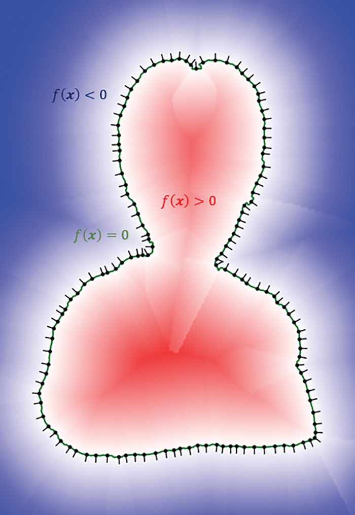
Figure 2: The color map of a field f(x) and the two-dimensional curve defined as f(x) = 0. Constraint points and normal vectors are represented by dots and short line segments respectively. The example is generated using the grid of the polynomial approach [13,14]

Existing work on implicit representations can be divided into two categories, namely, traditional mathematical methods and newly proposed learning-based methods. A typical traditional method is to generate the field f(x) as a linear combination of radial basis functions so that the zero-value set of the field satisfies the interpolation or approximation conditions [17–19]. In the multilevel partition of the unity approach [20], the field is generated as a weighted sum of hierarchical polynomials approximating signed distance functions (SDFs). The hierarchical structure greatly enhanced the capability of numerous input points. Another approach is to use Fourier series [21] and wavelets [22] to generate fields as indicator functions, where the value is one inside the surface and zero outside the surface. The Poisson surface reconstruction [9] replaces the function generation process with a Poisson equation with hierarchical local bases and is noise resistant. The grid of polynomial approach [13,14] generates fields as a set of polynomials that approximate the SDF condition. The simplicity of the function helps in the fast direct rendering of the surfaces. See comprehensive surveys [23,24] for detail.

More recently, deep learning-based approaches have gained more popularity. In those approaches, SDFs [25–28] or occupancy fields [29–32] are learned via machine learning methods. In [25,33], estimated projection vectors are obtained using deep learning methods, such as regression forests [34]. The sign can be calculated using the projection vector and surface normal. Finally, the signed projection vectors can be used to approximate SDFs. Moreover, the surfaces can be represented with decision boundaries retrieved from neural networks [35]. In this approach, an occupancy network is constructed, and the probability of either taking zero or one at an arbitrary point is output. The occupancy field consists of zeros and ones based on the higher probability at the corresponding location. The shape is represented by the decision boundary that separates zeros and ones. Different forms of the expected shape, such as point clouds, predefined models, or images, can be used as input. A state-of-the-art survey is provided in [36].

Although some methods for creating implicit shapes have been proposed, the problem of irregular parts is a typical issue, as mentioned in Section 1. Our approach is to restore irregular surfaces a posteriori according to the interactive operations of users. There are some methods for modifying implicit surfaces interactively. An implicit surface manipulation method, known as WarpCurves [37], has been proposed. This method allows users to modify surfaces by manipulating user-specific curves on surfaces. Another approach for deforming implicit surfaces is free-form deformation [38]. In this method, the field is updated according to control points or curves specified on surfaces. An interactive manipulation approach based on typical mathematical operations, such as Boolean, blending, twisting, and bending, has also been proposed [39]. Various deformations can be performed as a combination of simple operations and real-time rendering. Our method focuses on restoration of unexpectedly generated shapes and is designed to effectively remove irregular parts, including redundant protrusions and jaggy noise, using simple operations. The restoration level can also be controlled by user-specific parameters. The geometric information that users should provide is only masks that cover the irregular parts. The next section discusses the reasons for each type of issue.

3  The Issue

One of the common challenges in model creation is irregular parts that are unexpectedly generated, including curvature shaped redundant bulges and unexpectedly generated high frequency components. Defects such as missing points or unevenly displaced normal vectors may cause noisy or redundant problems. In this case, the interpolation may be misguided, resulting in either large curvatures or high-frequency components. As a result, redundant protruding parts or noisy parts are produced. Figs. 3 and 4 show some examples.

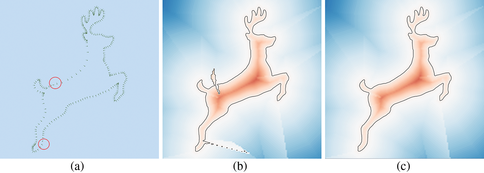
Figure 3: An example of redundant parts caused by the wrong direction of normal vectors, generated using the grid of polynomial approach [13,14]. Irregular directions of normal vectors are shown in (a). An irregular curve f(x) = 0 is shown in (b), and the ideal curve is shown in (c)

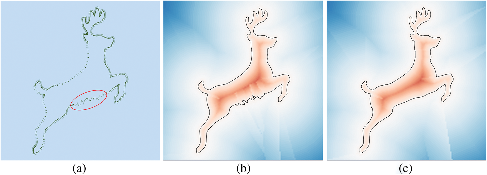
Figure 4: An example of a noisy curve, generated using the grid of polynomial approach [13,14]. Fluctuated distribution of normal vectors is shown in (a); the irregular curve f(x) = 0 is shown in (b), and the ideal curve is shown in (c)

4  Proposed Methods

This section presents implicit surface restoration methods that remove unexpectedly generated redundant protrusions and jaggy noise. Assuming a scalar field, f(x), is given in a bounding box ΩBB and the surface, f(x)=0, has some unexpected defects. The goal is to obtain a new scalar field, g(x), defined in ΩBB so that the surface, g(x)=0, is defect-free. The basic concept of our correction is to replace the field with a new one locally in the region surrounding the defects. Assuming a user-specific region Ωmask⊂ΩBB that covers the defect as a 2D illustration is shown in Fig. 5, which shows some examples of a mask at the specified location where the redundant protruding component should be removed. In our approach, the original field is replaced with a new one so that the defects are appropriately removed. The new field is generated in such way that the values are approximately equivalent to the rest of the mask, i.e.,

g(x){≈f(x)(x∈ΩBB∖Ωmask)=h(x)(x∈Ωmask),(1)

where h(x) is the newly generated field in the mask. Simultaneously, g(x) should be continuous at the boundary of the mask.

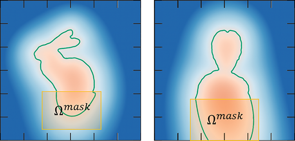
Figure 5: Illustrations of user-interactive specifications. To specify the mask, the user is expected to input the coordinate of the lower-left and the upper-right vertice of the mask

4.1 Correction of Redundant Parts

The strategy of removing redundant parts is illustrated in Fig. 6. Assuming f(x)=0 denotes an implicit shape with redundant parts. The goal is to define a new field, g(x), as an alternative to the given field, f(x). A standard situation occurs when the protruding part does not exceed the boundary of ΩBB, while a particular situation occurs when the protrusion touches one or more of the boundaries of ΩBB, and the mask touches the corresponding boundary. In this case, special care will be necessary, as discussed later in this section. The left and right illustrations in Fig. 5 show the standard and special situations, respectively, with corresponding mask specifications. The first step is to obtain a local field h(x) (x∈Ωmask) that appropriately removes the redundant protrusions. Assuming the rectangular mask is placed around a protrusion so that one edge is penetrated by the base of the protrusion as shown in Fig. 5. In an ideal situation, the new local field should possess the following three properties:

P1: the field is as smooth as possible.

P2: the value is equivalent to f(x) at the boundary of the mask for continuity.

P3: the value decays rapidly from positive to negative at the edge penetrated by the base.

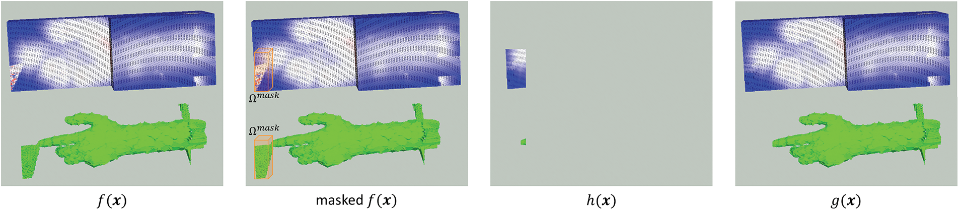
Figure 6: The strategy to remove redundant parts, a cuboid mask has been specified. The cross-section of the fields and the implicit surfaces are shown at the upper and lower part of the figures, respectively

The property P3 is to control the speed of decay. In this approach, it is assumed that some protruded surfaces are unexpectedly generated as the result of limitations on scanning environment. It means that users can specify the flatness of the restored surfaces after removing the protrusions by controlling the speed of the decay.

To obtain a field that mostly satisfies the three properties, we propose the following equations:

{min∫Ωmask(Δh(x))2dΩh(x)=f(x)(x∈∂Ωmask),∂h(x)∂n=α(x∈Emask)(2)

where ∂Ωmask is the boundary of the mask, Emask is the edge penetrated by the base of the protrusion, and α is a user-specific parameter that determines the gradient of the field at the edge. The first, second, and third equations correspond to P1, P2 and P3, respectively. In the first item, the field h(x) is the solution to Laplace’s equation if the minimum value is zero. Unfortunately, Laplace’s solution cannot be obtained because the second and third conditions are overdetermined. We adopt the least-square problem instead of Laplace’s equations to obtain a solution that is as smooth as possible under the overdetermined conditions. The second equation is the condition of continuity, which serves as the Dirichlet boundary condition in the context of solving the partial differential equation. The third one is the condition that determines the gradient of h(x) at Emask, which serves as the Neumann boundary condition. If α is large, the value rapidly decays toward the negative, and the zero-level set should be close to the edge. The reverse is also true. This means that α plays the role of controlling the roundness of the restored shape after removing the redundant protrusion. Fig. 7 shows the relationship between the parameter α and the effects of restoration of 2D examples.

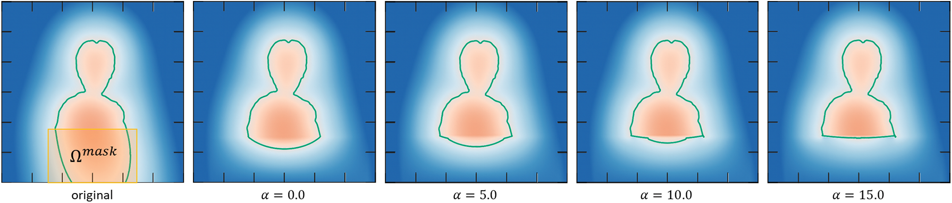
Figure 7: Different roundness of restored shapes obtained by setting different gradients of the field at the top edge of the mask. The examples are generated via Turk’s method [17]

In some special situations, the surface unexpectedly extends toward the border of ΩBB, and the mask should touch the border, as shown in Fig. 5 (right). In this case, the least-square problem lacks Dirichlet boundary condition at the border. Therefore, the function value should be determined along the border before solving the equations. A natural approach will be used to determine the values as the linear interpolation of an edge of f(xleft) and f(xright), where xleft and xright are the ends of the edge at the border. In 3D situations, assuming the bottom surface lakes Dirichlet boundary condition, it is to be determined by the mean value of the interpolation of the edge of f(xleft) and f(xright) and, the interpolation of the edge of f(xfront) and f(xrear).

For practical computations, the above-mentioned formulation should be appropriately discretized. We apply a finite difference scheme to obtain the discrete linear least-square equations. Assuming the domain ΩBB is divided into L×M×N uniform cells whose centers are xijk (i=1,2,…,L,j=1,2,…,M,k=1,2,…,N) and a mask Ωmask is placed so that the protrusion to be removed penetrates the top edge of the mask. Let IMIN and IMAX be the minimum and maximum indices of the discrete points within the mask Ωmask along the x-axis, respectively. Let JMIN and JMAX be the minimum and maximum indices of the discrete points within the mask Ωmask along the y-axis, respectively. Let KMIN and KMAX be the minimum and maximum indices of the discrete points within the mask Ωmask along the z-axis, respectively. The goal is to obtain the discrete values of the restored function, g(x), i.e.,

gijk={fijk(xijk∉Ωmask)hijk(xijk∈Ωmask),(3)

where fijk=f(xijk). At this moment, we have m unknown variables, where m=(IMAX−IMIN+1)×(JMAX−JMIN+1)×(KMAX−KMIN+1) and we will determine the unknowns hijk using the Eq. (2). With the abovementioned discretization, (2) can be discretized using a standard finite difference scheme as the following equations:

{minhijk∑i=IMINIMAX∑j=JMINJMAX∑k=KMINKMAX(hi−1,j,k+hi+1,j,k+hi,j−1,k+hi,j+1,k+hi,j,k−1+hi,j,k+16)2hijk=fijk(i∈{IMIN−1,IMAX+1}orj∈{JMIN−1,JMAX+1}ork∈{KMIN−1,KMAX+1}).hijKMAX=fijk−αd(i=IMIN,IMIN+1,…,IMAX,j=JMIN,JMIN+1,…,JMAX)(4)

where the notation d is the distance between the centers of neighboring cells. The discrete values at the top row in the mask, hijKMAX (IMIN≤i≤IMAX;JMIN≤j≤JMAX), can be determined only by the third equation. Therefore, we have n remaining unknowns where n=(IMAX−IMIN+1)×(JMAX−JMIN+1)×(KMAX−KMIN), and the discrete Eq. (4) leads to an overdetermined linear least-square system:

minh‖Ah−b‖2(A∈Rm×n),(5)

where h is the vector of n unknowns and b is the vector of m constants corresponding to m equations. Note that m>n.

The uniqueness of the least-square solution is critical. As a result, the solution is guaranteed to be unique, as described below. According to Eq. (4), the matrix A contains n rows that are identical to Laplace’s equation with the Dirichlet condition on the whole boundary, which has a unique solution. This means that the rank of the matrix is n. In other words, the matrix is full rank. Based on the basic properties of linear algebra, the overdetermined least-square problem with a full rank matrix has a unique solution. This means that although there are different least-square solvers, they all produce the same solution if they are accurate.

Another issue is the choice of least-square solvers. Typically, singular value decompositions (SVD), QR and conjugate gradient least squares (CGLS) are used to solve linear least square problems [40]. In this study, the matrix is sparse and might be quite large depending on the size of the mask and the resolution of the discretization. The algorithms of SVD and QR use dense matrices and are inappropriate for users because they require a significant amount of computational time and memory space. However, the CGLS matches our case because the algorithm is designed for sparse and large matrices. Therefore, we adopt CGLS as the least-square solver throughout this paper.

All restored discrete values in Eq. (3) can be obtained by solving the least-square problem. Finally, the restored field, g(x), can be obtained as the standard spline interpolation [13,14] of the discrete values gijk, i.e.,

g(x)=∑i∑j∑kcijkBi(x)Bj(y)Bk(z)(x=(x,y,z)∈ΩBB),(6)

where Bi(t) is a quadratic B-spline function with uniform intervals and cijk are the spline coefficients. Note that spline interpolation is not the only option and there are other ways like tri-linear interpolation and radial basis functions. We applied spline interpolation because the scaler values are given at uniform grid points and a smooth interpolation can be performed using an efficient scheme described in [13]. In conclusion, Fig. 8 shows the complete procedure of removing redundant parts. For more concise presentation of discrete filed fijk and gijk, the illustrations are given in 2D form.

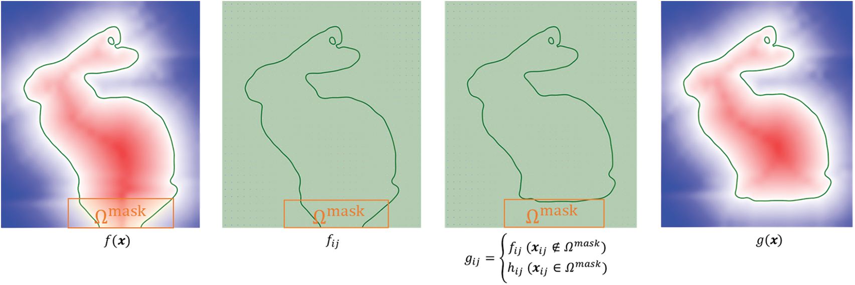
Figure 8: Illustration of the proposed algorithm of removing redundant parts

4.2 Correction of Noisy Parts

Assuming the shape, f(x)=0, contains partially generated jaggy noise and a user-specific mask, Ωmask, covering the noise. The goal is to define a new field, g(x), as Eq. (1). In this situation, the values of f(x) vary slightly about the noisy surface. Our main idea is to smooth out the small fluctuations in the user-specific mask via coarse sampling. To obtain the final function, g(x), which is continuous and smooth along the boundary of Ωmask, we perform fine sampling and spline interpolation over the entire domain. The following is the mathematical formulation of the idea. Let (mmask,nmask) be a user-specific sampling resolution of the mask, xijkmask be the sampling points, and fijkmask=f(xijkmask). We define the restored function, h(x) (x∈Ωmask), as the standard spline interpolation of fijkmask, i.e.,

h(x)=∑i∑j∑kcijkmaskBi(x)Bj(y)Bk(z)(x=(x,y,z)∈Ωmask),(7)

where Bi(t) is the quadratic B-spline with uniform intervals and cijkmask are the coefficients of the spline interpolation.

Currently, we have h(x) and f(x) inside and outside the mask, respectively. The two functions have gaps along the boundary of Ωmask, as shown in Fig. 9, and they must be smoothly connected. Let xijk be fine uniform sampling points over ΩBB. We then define the final function, g(x), as the spline interpolation of the fine sampling of the two functions, i.e.,

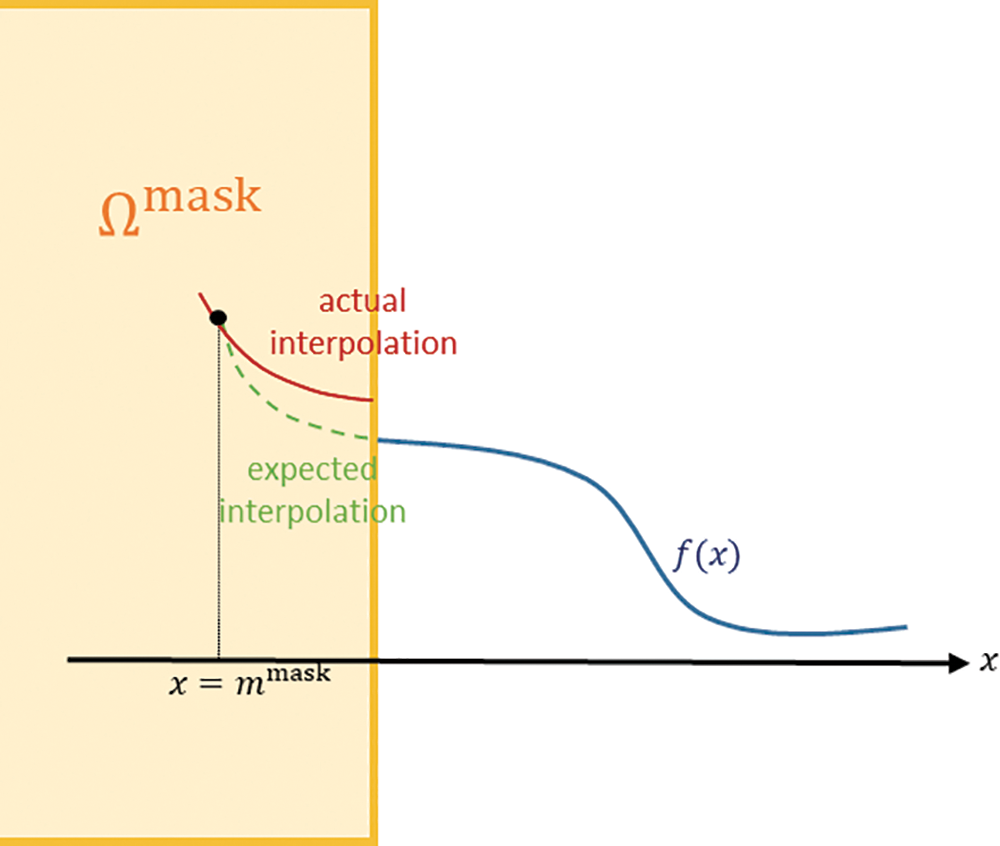
Figure 9: Illustration of the discontinuous gap at ∂Ωmask

gij={f(xijk)(xijk∈ΩBB∖Ωmask)h(xijk)(xijk∈Ωmask),(8)

g(x)=∑i∑j∑kcijkBi(x)Bj(y)Bk(z)(x=(x,y,z)∈ΩBB),(9)

where cijk are the coefficients of the spline interpolation of gijk. Fig. 10 shows the procedure of de-noise. Smoothing should be applied only to the mask while the detailed shape outside the mask keeps the original one. The smoothing intensity is controlled by the parameters, mmask and nmask. Fig. 11 shows the relationship between the parameters and the smoothing effects. For more concise illustration, they are given in 1D or 2D form.

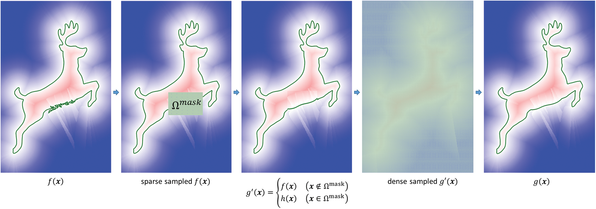
Figure 10: Illustration of the proposed algorithm of noise reduction

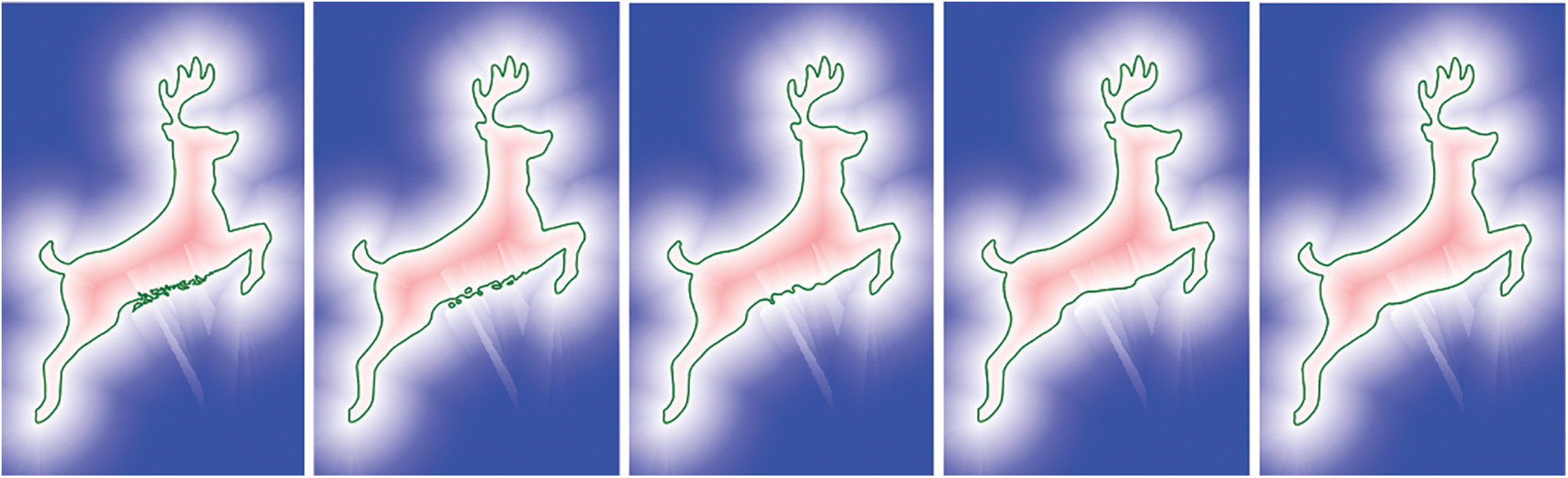
Figure 11: Examples of de-noise processes with different sparse sampling resolutions. From left to right: noised curve, de-noised curve applied 32 × 32, 16 × 16, 8 × 8 and, 4 × 4 discrete samples, respectively, in sparse sampling

5  Experiments

This section presents some experimental examples to evaluate the proposed methods. Three-dimensional restoration examples are provided, using methods discussed in Section 4 and extended to three-dimensional formulations. Fig. 12 shows the data points of “Venus,” “Nefertiti,” and “Happy Buddha.” The implicit surfaces are generated using the grid of polynomial approach [13,16].

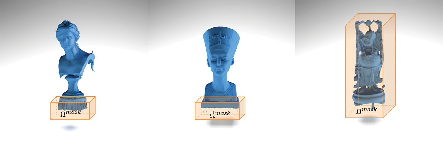
Figure 12: Test examples of a surface with irregular parts with respective mask specification. Left: surface “Venus” with the redundant part. Middle: Surface “Nefertiti” with noise part; the data point set is provided by Rapidform (INUS Technology, Inc., USA) [41]. Right: surface “Happy Buddha” with noisy parts around the entire domain; the data point set is provided by Stanford 3D Scanning Repository

Fig. 13 shows restoration examples of removing redundant parts. The redundant part is considered as the protruding part at the bottom of the statue “Venus,” and the user-specified mask covers this area. With different settings of the gradient α at the top surface of the specified mask, different shapes of restoration can be obtained. A flat shape can be obtained if a larger number of the gradient α is used, as shown in Fig. 13 (left), whereas a shape with larger roundness can be obtained if the gradient α is getting smaller, as shown in Fig. 13 (right).

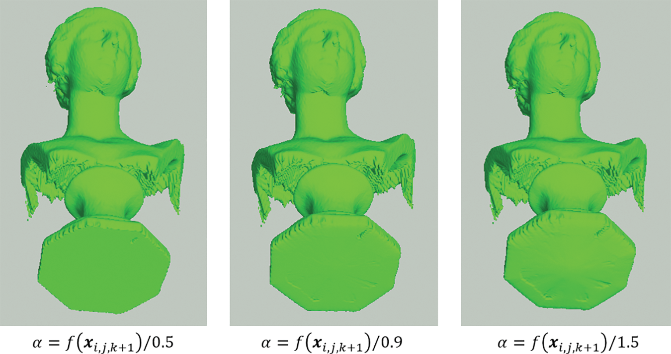
Figure 13: Examples of removing redundant parts

Figs. 14 and 15 show restoration examples of partial and overall de-noise, respectively. The resolution of coarse sampling influences the intensity of de-noise, and setting a smaller number of sampling density results in a larger intensity of de-noise. However, the proposed method works well only when there are only a few smaller noisy parts, as shown in Fig. 14, in which case only a smaller mask is required to make corrections. If a de-noise process across the entire domain is required, the proposed method is less robust because it is difficult to control the intensity of de-noise to provide a well-balanced setting capable of removing noisy parts while preserving other details. As a result, there is a trade-off between the details of restoration and the intensity of de-noise. This limitation is vital in the case shown in Fig. 15.

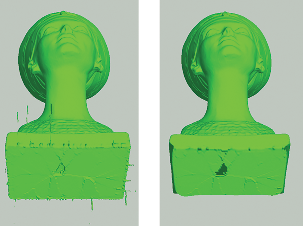
Figure 14: Examples of removing noisy components around a small region at the bottom of the statue. The original and restored surfaces are given by the left and right figures, respectively. The density of sparse sampling is (30, 30, 30)

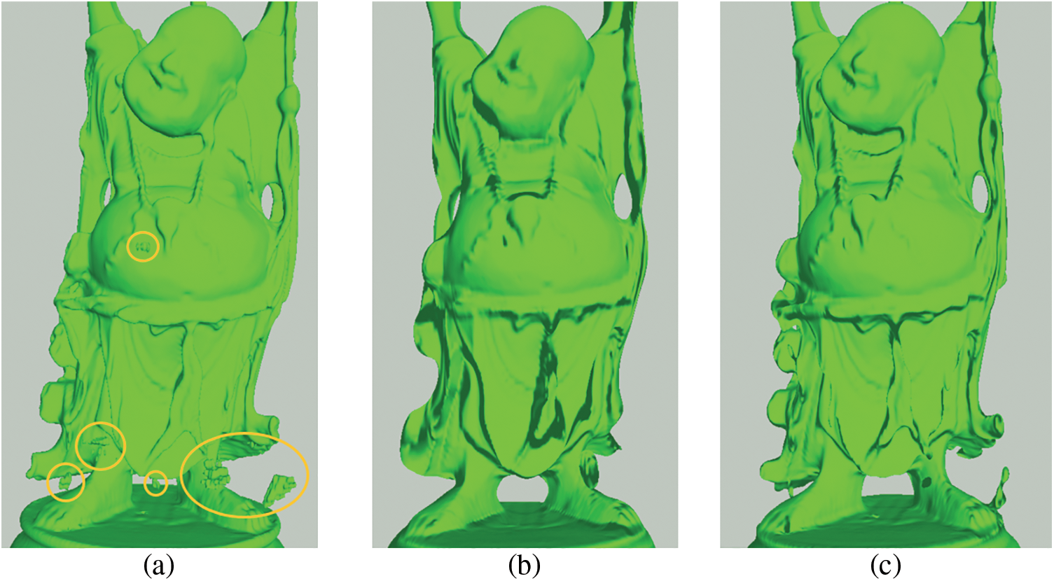
Figure 15: Examples of the overall processing of de-noise. The original surface is shown in (a). Less-detailed with higher de-noise intensity is given in (b), after setting coarse sampling resolution as (20, 20, 20). Noisy parts have not been completely removed in (c), after setting coarse sampling resolution as (40, 40, 40), but overall details have been well-preserved

6  Conclusion and Future Work

This paper presents many methods to correct three-dimensional implicit surfaces with irregular components, such as redundant protruding parts and jaggy noise. Sections 1 and 2 introduce implicit surfaces and some state-of-the-art generation methods. Section 3 offers observations of irregular parts and their respective causes. Section 4 introduces the proposed correction methods. Experiments in Section 5 demonstrates that the proposed approaches can produce effective corrections, subject to some limitations that will be described further below.

In most situations, users have little knowledge regarding the properties of the field f(x). Good restoration requires the use of appropriate parameters, such as α and the coarse sampling resolution. On the parameter α, the value should be determined depending on the users’ requirements. Although visualizing the restored shape will help users to control the parameter, such interface is not developed at this moment and this is an important future work. The same problem applies to the parameter of sampling resolution. In addition, developing 3D GUIs to set masks visually will strongly support the users and this is considered as another important future work. For other limitations, the trade-off between the intensity of noise reduction and the level of restored details discussed in Section 5 has theoretically narrowed down the effectiveness of the proposed method.

Moreover, the proposed methods output the final result, g(x), interpolated by spline, in Eqs. (6) and (9). Such an operation will make the result differ from the original field f(x) outside the mask if the original field is generated by other methods. However, in general, such a difference is minimal and we can consider g(x) as a decent approximation of the original field f(x).

Funding Statement: This work was supported by JSPS KAKENHI Grant No. 21K11928.

Conflicts of Interest: The authors declare that they have no conflicts of interest to report regarding the present study.

References

1. Schmidt, R., Wyvill, B., Galin, E. (2005). Interactive implicit modeling with hierarchical spatial caching. International Conference on Shape Modeling and Applications 2005 (SMI' 05), pp. 104–113. https://doi.org/10.1109/SMI.2005.25 [Google Scholar] [CrossRef]
2. Marschner, S., Shirley, P., Ashikhmin, M., Gleicher, M., Hoffman, N. et al. (2015). Fundamentals of computer graphics. 4th edition. USA: A K Peters/CRC Press. [Google Scholar]
3. Kanetsuki, Y., Nakata, S. (2015). Moving particle semi-implicit method for fluid simulation with implicitly defined deforming obstacles. Journal of Advanced Simulation in Science and Engineering, 2(1), 63–75. https://doi.org/10.15748/jasse.2.63 [Google Scholar] [CrossRef]
4. Kanetsuki, Y., Nakata, S. (2020). Artificial force free boundaries: Particle-based fluid simulation with implicit surfaces. In: Computational and experimental simulations in engineering, pp. 207–222. Springer, Cham, Switzerland. https://doi.org/10.1007/978-3-030-27053-7_20 [Google Scholar] [CrossRef]
5. Sonon, B., François, B., Massart, T. J. (2015). An advanced approach for the generation of complex cellular material representative volume elements using distance fields and level sets. Computational Mechanics, 56(2), 221–242. https://doi.org/10.1007/s00466-015-1168-8 [Google Scholar] [CrossRef]
6. Yang, N., Wang, S., Gao, L., Men, Y., Zhang, C. (2017). Building implicit-surface-based composite porous architectures. Composite Structures, 173(4), 35–43. https://doi.org/10.1016/j.compstruct.2017.04.004 [Google Scholar] [CrossRef]
7. Parulek, J., Viola, I. (2012). Implicit representation of molecular surfaces. 2012 IEEE Pacific Visualization Symposium, pp. 217–224. Songdo. [Google Scholar]
8. Liu, Y., Song, Y., Yang, Z., Deng, J. (2017). Implicit surface reconstruction with total variation regularization. Computer Aided Geometric Design, 52(5), 135–153. https://doi.org/10.1016/j.cagd.2017.02.005 [Google Scholar] [CrossRef]
9. Kazhdan, M., Bolitho, M., Hoppe, H. (2006). Passion surface reconstruction. Symposium on Geometry Processing, pp. 61–70. Cagliari. https://doi.org/10.2312/SGP/SGP06/061-070 [Google Scholar] [CrossRef]
10. Wang, J., Yu, Z., Zhu, W., Cao, J. (2013). Feature-preserving surface reconstruction from unoriented, noisy point data. Computer Graphics Forum, 32(1), 164–176. https://doi.org/10.1111/cgf.12006 [Google Scholar] [CrossRef]
11. Liu, S., Wang, C. C. L. (2012). Quasi-interpolation for surface reconstruction from scattered data with radial basis function. Computer Aided Geometric Design, 27(7), 435–447. https://doi.org/10.1016/j.cagd.2012.03.011 [Google Scholar] [CrossRef]
12. Drake, K. P., Fuselier, E. J., Wright, G. B. (2022). Implicit surface reconstruction with a curl-free radial basis function partition of unity method. arXiv: 2101.05940. [Google Scholar]
13. Nakata, S., Aoyama, S., Makino, R., Hasegawa, K., Tanaka, S. (2012). Real-time isosurface rendering of smooth fields. Journal of Visualization, 15(2), 179–187. https://doi.org/10.1007/s12650-011-0119-5 [Google Scholar] [CrossRef]
14. Itoh, T., Nakata, S. (2015). Fast generation of smooth implicit surface based on piecewise polynomial. Computer Modeling in Engineering & Sciences, 107(3), 187–199. https://doi.org/10.3970/cmes.2015.107.187 [Google Scholar] [CrossRef]
15. Vemuri, B., Bolle, R. (1991). On three-dimensional surface reconstruction methods. IEEE Transactions on Pattern Analysis & Machine Intelligence, 13(1), 1–13. https://doi.org/10.1109/34.67626 [Google Scholar] [CrossRef]
16. Poursaeed, O., Fisher, M., Aigerman, N., Kim, V. G. (2020). Coupling explicit and implicit surface representations for generative 3D modeling. In: Lecture notes in computer science, vol. 12355, pp. 667–683. Springer, Cham, Switzerland. https://doi.org/10.1007/978-3-030-58607-2_39 [Google Scholar] [CrossRef]
17. Turk, G., O'Brien, J. F. (2002). Modelling with implicit surfaces that interpolate. ACM Transactions on Graphics, 21(4), 855–873. https://doi.org/10.1145/571647.571650 [Google Scholar] [CrossRef]
18. Carr, J. C., Beatson, R. K., Cherrie, J. B., Mitchell, T. J., Fright, W. R. et al. (2001). Reconstruction and representation of 3D objects with radial basis functions. Proceedings of the 28th annual conference on Computer Graphics and interactive techniques (SIGGRAPH ’01), pp. 67–76. Los Angeles. [Google Scholar]
19. Zeng, Y., Zhu, Y. (2022). Implicit surface reconstruction based on a new interpolation/approximation radial basis function. Computer Aided Geometric Design, 92(4), 102062. https://doi.org/10.1016/j.cagd.2021.102062 [Google Scholar] [CrossRef]
20. Ohtake, Y., Alexander, B., Alexa, M., Turk, G., Seidel, H. P. (2003). Multi-level partition of unity implicits. ACM Transactions on Graphics, 22(3), 463–470. https://doi.org/10.1145/882262.882293 [Google Scholar] [CrossRef]
21. Kazhdan, M. (2005). Reconstruction of solid models from oriented point sets. Proceedings of the Third Eurographics Symposium on Geometry Processing (SIGGRAPH ’05), pp. 73–82. Vienna. [Google Scholar]
22. Manson, J., Petrova, G., Schaefer, S. (2008). Streaming surface reconstruction using wavelets. Computer Graphics Forum, 27(5), 1411–1420. https://doi.org/10.1111/j.1467-8659.2008.01281.x [Google Scholar] [CrossRef]
23. Berger, M., Levine, J. A., Nonato, L. G., Taubin, G., Silva, C. T. (2013). A benchmark for surface reconstruction. ACM Transaction on Graphics, 32(2), 1–17. https://doi.org/10.1145/2451236.2451246 [Google Scholar] [CrossRef]
24. Berger, M., Tagliasacchi, A., Seversky, L. M., Alliez, P., Guennebaud, G. et al. (2017). A survey of surface reconstruction from point clouds. Computer Graphics Forum, 36(1), 301–329. https://doi.org/10.1111/cgf.12802 [Google Scholar] [CrossRef]
25. Erler, P., Guerrero, P., Ohrhallinger, S., Mitra, N. J., Wimmer, M. (2020). Points2Surf: Learning implicit surfaces from point clouds. European Conference on Computer Vision, pp. 108–124. Glasgow. [Google Scholar]
26. Liu, S., Guo, H., Pan, H., Wang, P., Tong, S. et al. (2021). Deep implicit moving least-squares functions for 3D reconstruction. Proceedings of the IEEE Conference on Computer Vision and Pattern Recognition, pp. 1788–1797. [Google Scholar]
27. Ma, B., Han, Z., Liu, Y., Zwicker, M. (2021). Neural-pull: Learning signed distance functions from point clouds by learning to pull space onto surfaces. Proceedings of the 38th International Conference on Machine Learning, pp. 7246–7257. [Google Scholar]
28. Ma, B., Liu, Y., Han, Z. (2022). Reconstructing surfaces for sparse point clouds with on-surface priors. Proceedings of the IEEE/CVF Conference on Computer Vision and Pattern Recognition, pp. 6315–6325. New Orleans. [Google Scholar]
29. Jia, M., Kyan, M. (2010). Learning occupancy function from point clouds for surface reconstruction. arXiv: 11378. [Google Scholar]
30. Martel, J. N. P., Lindell, D. B., Lin, C. Z., Chan, E. R., Monteiro, M. et al. (2021). ACORN: Adaptive coordinate networks for neural scene representation. arXiv: 2105.02788. [Google Scholar]
31. Peng, S., Niemeyer, M., Mescheder, L., Pollefeys, M., Geiger, A. (2020). Convolutional occupancy networks. European Conference on Computer Vision, pp. 523–540. Glasgow. [Google Scholar]
32. Takikawa, T., Litalien, J., Yin, K., Kreis, K., Loop, C. et al. (2021). Neural geometric level of detail: Real-time rendering with implicit 3D shapes. arXiv: 2101.10994. [Google Scholar]
33. Ladický, L., Saurer, O., Jeong, S., Maninchedda, F., Pollefeys, M. (2017). From point clouds to mesh using regression. 2017 IEEE International Conference on Computer Vision (ICCV), pp. 3913–3922. Venice. [Google Scholar]
34. Breiman, L. (2001). Random forests. Machine Learning, 45(1), 5–32. https://doi.org/10.1023/A:1010933404324 [Google Scholar] [CrossRef]
35. Mescheder, L., Oechsle, M., Niemeyer, M., Nowozin, S., Geiger, A. (2019). Occupancy networks: Learning 3D reconstruction in function space. Proceedings of the IEEE/CVF Conference on Computer Vision and Pattern Recognition (CVPR), pp. 4460–4470. Long Beach. [Google Scholar]
36. Huang, Z., Wen, Y., Wang, Z., Ren, J., Jia, K. (2022). Surface reconstruction from point clouds: A survey and a benchmark. arXiv: 2205.02413. [Google Scholar]
37. Sugihara, M., Wyvill, B., Schmidt, R. (2010). WarpCurves: A tool for explicit manipulation of implicit surfaces. Computers & Graphics, 34(4), 282–291. https://doi.org/10.1016/j.cag.2010.03.008 [Google Scholar] [CrossRef]
38. Eyiyurekli, M., Breen, D. (2010). Interactive free-form level-set surface-editing operators. Computers & Graphics, 34(5), 621–638. https://doi.org/10.1016/j.cag.2010.06.006 [Google Scholar] [CrossRef]
39. Reiner, T., Mückl, G., Dachsbacher, C. (2011). Interactive modeling of implicit surfaces using a direct visualization approach with signed distance functions. Computers & Graphics, 35(3), 596–603. https://doi.org/10.1016/j.cag.2011.03.010 [Google Scholar] [CrossRef]
40. Ascher, U. M., Greif, C. (2011). A first course in numerical methods. USA: Society for Industrial and Applied Mathematics. [Google Scholar]
41. Kim, D. B., Kang, E. C., Lee, K. H., Pajarola, R. B. (2006). Framework for adaptive sampling of point-based surfaces using geometry and color attributes. Proceedings of the International Conference on Computational Science, pp. 371–374. Reading, UK. [Google Scholar]
Cite This Article
Copyright © 2023 The Author(s). Published by Tech Science Press.
This work is licensed under a Creative Commons Attribution 4.0 International License , which permits unrestricted use, distribution, and reproduction in any medium, provided the original work is properly cited.
Downloads
Citation Tools