Multi-Stage Improvement of Marine Predators Algorithm and Its Application

1  Introduction

Metaheuristic Algorithms are studied relying on the combination of stochastic algorithms and local search algorithms. They can search globally and find similar solutions to the optimal solutions. These intelligent algorithms can be applied to solve real-life optimization problems [1]. Some of the intelligent algorithms are genetic algorithm (GA) [2], particle swarm optimization (PSO) [3], grey wolf optimizer (GWO) [4], artificial fish-swarm algorithm (AFSA) [5], artificial bee colony algorithm (ABC) [6], marine predators algorithm (MPA) [7] and so on. Compared to classical optimization algorithms, these algorithms have the advantages of being flexible, derivative independent as well as fast and efficient in dealing with discrete variables. The marine predators algorithm (MPA) is an intelligence algorithm inspired by the predatory behavior of marine species and was proposed by Faramarzi et al. in 2020 [7], which is a new algorithm that has recently attracted attention. In MPA, marine species can be in the two logical states of predator and prey at the same time. And this parallel mode improves the efficiency and accuracy of the optimization search. Currently it has been successfully applied to engineering optimization design, medical diagnosis, system optimization design etc.

The advantage of MPA over other algorithms is that the predator performs multiple motions depending on the behavior of the prey. According to the strategy of the best encounter, the predator can choose Levy motion or Brownian motion, which ensures the connection between predator and prey. Specifically, the Levy strategy is used by the predator when the number of prey in the area is low and on the contrary, the predator performs Brownian motion. The MPA is divided into three stages based on the speed score. The predator’s action pattern is regulated by using a segmented search strategy. At low velocity ratios (v=0.1), the predator performs Levy motion in order to search for the prey. At the same time the prey is in Brownian or Levy motion; at unit speed ratio (v=1), the predator chooses the appropriate strategy according to the movement of the prey. If the prey is stalking in the marine through Levy motion, Brownian motion by the predator is the best choice; at high speed ratio (v≥10), the best strategy for the predator is to be at rest, when the prey is in Brownian or Levy motion. In other words, the movement of the predator is determined by the concentration of the prey in the marine environment. Also, MPA has to take into account the influence of other factors in the environment, both natural and anthropogenic, which can change the behavior of predators and prey to affect the efficiency of the algorithm.

Although the global search capability of MPA is stronger than that of algorithms such as particle swarm optimization, it still suffers from weak convergence and easily falls into local optimum. In order to improve the performance of MPA in the search for optimization, many scholars have conducted a series of research on it. Houssein et al. [8] combined reinforcement learning (RL) with MPA and proposed a new method Deep-MPA. A new variant of the marine predator algorithm is called MPAmu [9]. The exploitation of MPA is enhanced by using an additional variant operator. A novel improved MPA (IMPA) [10] was proposed by Sowmya et al. It uses an opposition-based learning scheme and increases the diversity of populations. In addition, a modified MPA was investigated that was using chaotic reverse learning and adaptive update equations [11]. Both methods increased the diversity of populations and improved the efficiency of the algorithm operation. Elaziz et al. combined quantum theory with the algorithm and reprogrammed the multi-stage search strategy, which improved the exploration and exploitation of the algorithm [12]. Also, they applied the algorithm to the problem of multilayer image segmentation and obtained good results. In order to overcome the disadvantage of MPA, [13] proposed a Golden-Sine Dynamic Marine Predator Algorithm (GDMPA). Logistic-Logistic (L-L) cascade chaos and Golden-Sine facto were used to achieve a better balance between exploration and exploitation. Additionally, an enhanced marine predators algorithm, which is termed NMPA [14], with the neighborhood-based learning strategy and the adaptive population size strategy is proposed by Hu et al. A novel image segmentation algorithm based on the improved marine predators algorithm (MPA) is proposed. HMPA [15] is applied the linearly increased worst solutions improvement strategy (LIS) and ranking-based updating strategy (RUS), which could find better solutions efficiently.

The core of metaheuristic algorithms is exploration and exploitation. Although MPA is a novel algorithm, it still has an imbalance between exploration and exploitation. Over-emphasis on exploration can lead to species moving too fast. Obviously, this approach tends to miss optimal solutions; over-emphasis on exploitation can lead to aggregation and stagnation of population, which can trap the algorithm in local optimal solutions. Balancing exploration and exploitation is the key to solving the algorithmic problems. No single algorithm can be suitable for all problems, or even for different stages of a problem. Drawing on the advantages of other algorithms and then combining MPA is also a popular research.

In this paper, we introduce the linear flight strategy and PSO search mechanism into MPA. The multi-stage search mechanism of MPA is retained, which is an irreplaceable advantage of other algorithms. In the first stage we keep the original Brownian motion, and the marine species are evenly and randomly spread over the search area. During the second stage, the first half of predators carry out a linear flight strategy and use it at a distance from the prey, thus increasing the chance of re-employment. The second half uses the search mechanism of PSO, which adds interaction between individuals and enhances the predator’s exploitation ability. The third stage also uses this mechanism to speed up the convergence of the algorithm. In addition, this paper also uses self-adjusting weight updates to adjust the parameters, so that the performance of the algorithm can be improved.

This paper is organized as follows. Section 2 reviews the classical marine predators algorithm. Then, the innovative aspects of the MSMPA proposed in this paper are presented in Section 3. We describe the CEC2017 test functions and experimental setup which are used to analyze its experimental study and compared its performance with other algorithms in Section 4. It is also applied to a multidimensional nonlinear structural design optimization problem in Section 5. Finally, a short conclusion is given in Section 6, which contains a description of the MSMPA and a vision for the future.

2  Marine Predators Algorithm

2.1 Brownian Motion

Brownian motion is a common type of irregular motion that is manifested by cluttered and disordered particles. The particles in life are usually suspended in a liquid or gas. Mathematically, Brownian motion is a random variable that follows a normal distribution, and it is also a Markov process. Its step size is a probability function defined by a Gaussian distribution. The control density function of the point of motion x is given by

fB(x;μ,σ)=12πσ2exp⁡(−(x−μ)22σ2)=12πexp⁡(−x22)

where the mean μ is 0 and the unit variance σ2 is 1.

The trajectories of Brownian motion in 2D and 3D space are depicted in Fig. 1. Fig. 1b shows the 2D trajectories of Brownian motion and 3D space is showed in Fig. 1c. From the figures, we can see that Brownian motion is random and extensive in space, which has uniform and controllable step lengths. This means that Brownian motion is more suitable for the pre-path of marine creatures and it is easy to expand the range of random positions of predators and prey in the region.

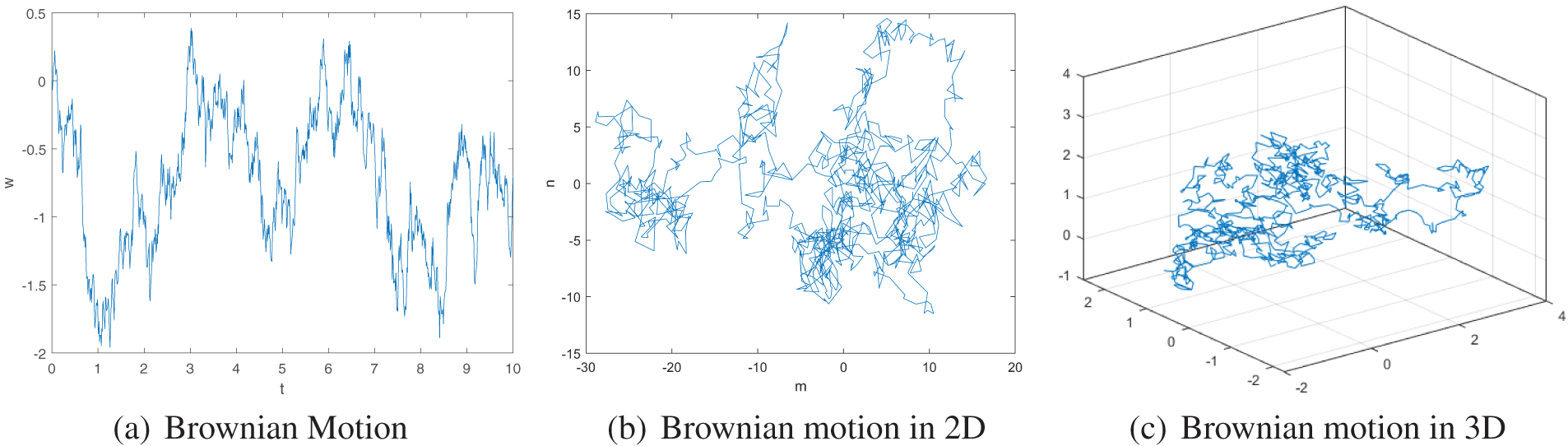
Figure 1: Brownian motion

2.2 Levy Motion

Levy flight was proposed by the French mathematician Levy [16] as a stochastic wandering model. It is a Markov process like Brownian motion. Levy flight is characterized by stochastic large probability short-distance exploration and small probability long-distance exploration. The trajectory of Levy process is shown in the Fig. 2. It was shown in [17,18] that Levy movement is used as a foraging and light-seeking strategy for many animals in nature, including marine species.

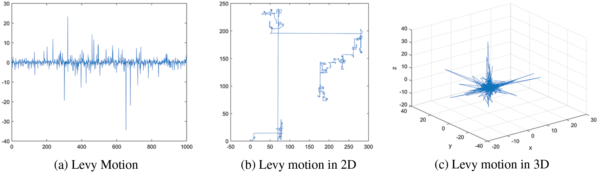
Figure 2: Levy motion

fLevy=η|v|−γ(1)

The parameter γ=1.5 is the power-law component; η and v obey the normal distribution.

{η∼N(0,ση2)v∼N(0,σv2)(2)

The standard deviation corresponding to the above equation satisfies the following equation.

{ση={Γ(1+γ)sin⁡(πγ2)Γ(1+γ2)×2(γ−1)/2×γ}σv=1(3)

Levy flight is considered to be the best search pattern for the algorithm when the number of prey in the environment is less in [19].

2.3 Update Strategies

At the beginning of the MPA, an Elite Matrix and a Prey Matrix are constructed. The Elite Matrix is used to store information about the best predators with the purpose of monitoring prey location information and finding other prey. The Elite Matrix is represented as follows:

Elite=[X1,1l⋯X1,Dl⋮⋱⋮XN,1l⋯XN,Dl]N×D(4)

where Xl→ is the elite predator vector. Unlike other intelligent algorithms, the population in the marine predators algorithm is composed of both predators and prey, of which there is an interchangeable relationship between predators and prey. If there is a better predator in the foraging process, the elite predator in the matrix will be replaced.

The prey is defined as another Prey matrix. The position of the predator is updated according to its formulation. Initializing the initial prey, where the predator constitutes the elite. The predator matrix is expressed as follows:

Prey=[X1,1l⋯X1,Dl⋮⋱⋮XN,1l⋯XN,Dl]N×D(5)

The MPA relies mainly on the update of the position information of these two matrices to complete the optimization process. The movement of the predator and prey in the MPA is divided into three phases with different velocities. The specific steps are as follows:

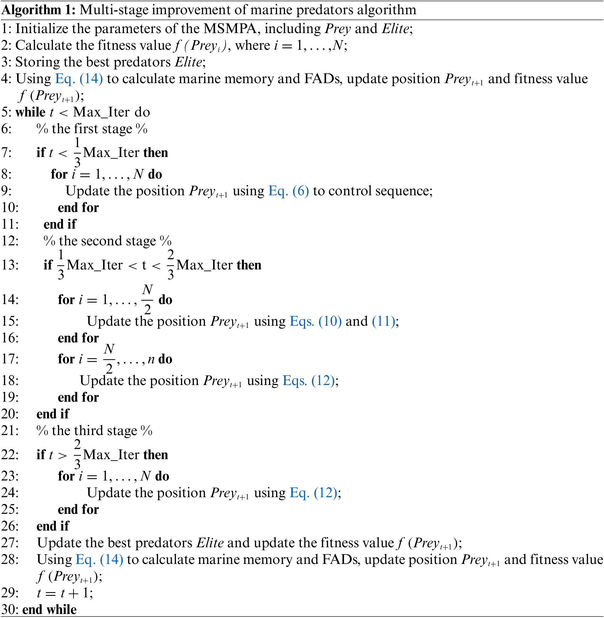
1.    The high speed ratio occurs mainly in the initial stage. And in order to coordinate the speed of the predator and prey, the best strategy for the predator is to be at rest in the case of a high speed ratio v≥10 or when the prey is moving faster than the predator. Specifically, as follows, improving the exploration ability of the population becomes a priority at this time.

Whilet<13Max_IterStepsizei→=RB→⊗(Elitei→−RB→⊗Preyi→)i=1,…,nPreyi→=Preyi→+P⋅R→⊗Stepsizei→(6)

where t denotes the current number of iterations and Max_Iter denotes the maximum number of iterations. RB→ denotes Brownian motion, and is a vector of random numbers based on a normal distribution. ⊗ represents the term-by-term multiplication and RB→ is multiplied with the prey to simulate the motion of the prey. P is a vector of uniform random numbers with a constant of 0.5 and R→ is a vector of uniform random numbers between [0,1]. Step 1 uses Brownian motion while increasing randomness. At this point the marine environment is expanded and the foraging chances of predators are greatly increased.

2.   With a unit speed ratio, predators and prey move at essentially the same speed. At this stage, creatures need to both maintain diversity and enhance interactivity. Both exploration and exploitation are key factors influencing predation. The prey is also a predator, so the prey is responsible for exploitation and the predator is responsible for exploration. According to the movement pattern of the species, at v/approx1, the Levy strategy is used by the prey to move, while at the same time Brownian movement is called the best strategy for the predator. So half of the population at this stage is represented as follows:

While13Max_Iter≤t≤23Max_IterStepsizei→=RL→⊗(Elitei→−RL→⊗Preyi→)i=1,…,n2Preyi→=Preyi→+P⋅R→⊗Stepsizei→(7)

where RL→ represents Levy motion, a vector of random numbers based on the Levy distribution. RL→⊗Preyi→ simulates the prey movement, and this part is responsible for the exploitation. The second half of the population in this stage is expressed as follows:

Stepsizei→=RB→⊗(RB→⊗Elitei→−Preyi→)i=n2,…,nPreyi→=Elitei→+P⋅CF⊗Stepsizei→CF=(1−IterMax_Iter)(2×IterMax_Iter)(8)

where CF is an adaptive parameter that controls the movement step of the predator, RB→ ⊗ Elitei→ indicates that the trajectory of the predator is a Brownian motion and the prey updates its position according to the movement of the predator.

3.   When the movement of the population reaches a low velocity ratio, it is necessary to improve the proximity search capability of the algorithm. So Levy motion is performed at the final stage in MPA.

Whilet>23Max_IterStepsizei→=RL→⊗(RL→⊗Elitei→−Preyi→)i=1,…,nPreyi→=Elitei→+P⋅CF⊗Stepsizei→(9)

where RL→⊗Elitei→ simulates the movement of the predator to help update the position of the prey.

3  Multi-Stage Improvement of Marine Predators Algorithm

3.1 Update Strategies

According to the movement strategy of the predator, the main idea of the algorithm is to be mainly responsible for the exploration in the early stage. The search space of the solution is expanded in the first stage. In the middle stage, exploration is gradually replaced by exploitation, where they are performed simultaneously. The later stage is mainly responsible for exploitation to avoid the predator moving too fast and so missing the global optimal solution. In this paper, we still use segmented processing to balance exploration and exploitation capabilities.

When marine species i is in the first half of the iterative process, the Brownian motion can cover the region with uniform and controlled steps. So all species in this stage simulate the prey for the original Brownian motion.

During the first half of the second stage, in order to enhance the interaction between species, we used the strategy of linear flight to guide they to move. There are two cases of linear flight: predators that are far from some prey will swim in a line towards the prey, that is, predators that are far from the global optimal position will move in a straight line. The formula is as follows:

Preyi→=λ⋅(Preyi→+ϕ⋅(Elitei→−Preyi→))(10)

Another case is that if the predators move to a terminal position beyond the optimal search area, the position is represented as

Preyi→=λ⋅(Preyi→+1ϕ⋅(Elitei→−Preyi→))(11)

where ϕ is the acceleration factor to control the convergence velocity. We set it to the golden ratio. λ is the scale factor, which is a standard uniformly distributed random number. The probability of the two linear motion cases is 0.5.

The second half of the search method of the predator transitions to exploitation, and the algorithm’s position update strategy differs for different search strategies and different iteration stages of the step. If the prey only performs Levy moves, it may lead to a similar behavior of all individuals falling into local optimal. When a predator stagnates and cannot leave this space using the random wandering strategy of Levy, it means that it cannot jump out of the local minimum using the position of the neighboring individuals, and then the population diversity decreases substantially, which is not conducive to population search. Therefore, in the other half of the second stage and the third stage, we use the search mechanism of PSO, which has a strong local merit-seeking ability.

C=(c1−c2)⋅Max_Iter−IterMax_Iter+c2ξ=1−IterMax_IterStepsizei→=ξ⋅Preyi→+C⋅rand→⋅(Elitei→−Preyi→)Preyi→=Elitei→+P⋅CF⋅Stepsizei→(12)

where c1=2.5, c2=0.5. C is reduced as the number of iterations is increased, which means that the population is progressively less influenced by individual optimality in the later stages of evolution. ξ is a weight factor. Similarly, the weight of Stepsize→ is gradually reduced as it evolves. At this point Prey gradually gathers around Elite and moves in small increments to find the optimal solution.

3.2 Self-Adjusting Weight

The search mechanism of PSO is utilized to reduce the randomness and uncertainty of marine species movement during the exploitation phase and accelerate the convergence of the algorithm. Meanwhile, we use self-adjusting weight for P to control the position update. The exploration capability of the algorithm is increased in the early stage, and the exploitation capability of the algorithm is enhanced in the later stage.

P=exp⁡(tan⁡(−π4⋅exp⁡IterMax_Iter))(13)

In summary, this paper provides a phased improvement of MPA. The Brownian motion in the pre-phase is still adopted to provide a comfortable predatory environment for marine species. The middle phase is carried out in two stages. In order to prevent predators and prey from overgathering or overdispersing, half of the species adopt a linear flight strategy. The PSO search mechanism with a very high level of interactivity is accepted by the other half. At the later stage, the creatures gather and roam around the prey, in search of the best prey. The PSO search mechanism is still adopted in order to search in the vicinity of the best individual in a small area, which allows the algorithm to converge well. At the same time, the constant P is replaced by self-adjusting weight. Updating the P parameter according to the state of the predation process can be better integrated into the predation process.

3.3 Vortex Formation and Fish Aggregation Devices (FADs) Effects

For the way of movement of marine creatures, the influence of the surrounding environment on it also needs to be considered. In the MPA algorithm, FADs are considered as the local optimal solution, which is needed to be found out. In the algorithm FADs effect is used to prevent the organisms from stopping their movement. It allows the fish to make longer distance jumps to make they active again. So the FADs are expressed as follows:

Preyi→={Preyi→+CF[Xmin→+R→⊗(Xmax→−Xmin→)]⊗U→ifr≤FADsPreyi→+[FADs(1−r)+r](Preyr1→−Preyr2→)ifr>FADs(14)

where r is a random number, FADs is a constant that affects the optimization process, and usually FADs=0.2. r1 and r2 are two random subscripts of Prey, 1≤r1,r2≤n. U is a binary vector containing 0 and 1, such that random is a random number between [0,1] and each element of Ui can be defined as

Ui={0ifrandom≤FADs1ifrandom>FADs(15)

3.4 Marine Memory

Marine memory is used to update the elite matrix. First, the fitness is calculated for the prey matrix. If the fitness of the prey is better than the corresponding result in the elite matrix, the individual is replaced, that is, the elite matrix is updated. Then the fitness of all individuals in the elite matrix is calculated to find the best individual. If it meets the requirements, the algorithm stops, otherwise it continues to iterate.

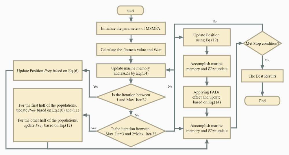
The pseudo-code for the MSMPA algorithm is given in Algorithm 1 and flowchart of MSMPA is shown in Fig. 3.

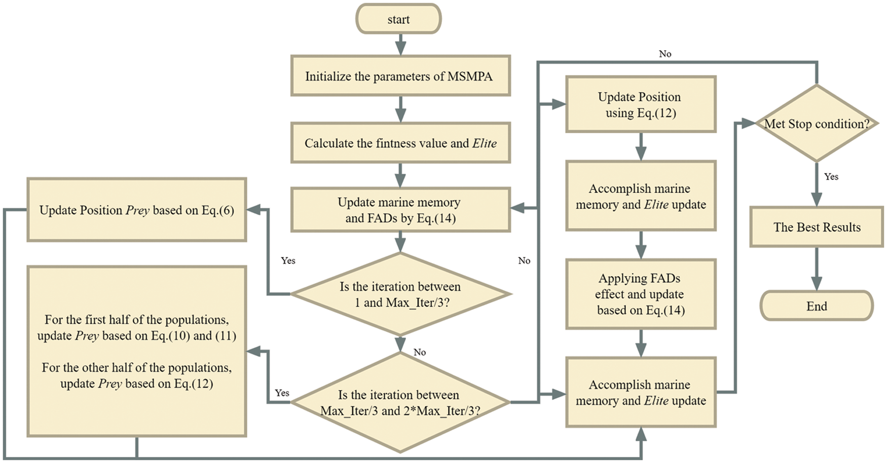
Figure 3: Flowchart of MSMPA

4  Experimental Verification and Analysis

4.1 Baseline Test Functions

In this paper, CEC2017 benchmark functions [13] are used to evaluate the performance of MSMPA. Among the 30 functions, 29 functions are selected for testing in this paper. F2 is excluded because it has strong instability, especially in multidimensional and high-dimensional problems. The benchmark functions of CEC2017 are divided into four main classes, including unimodal functions (F1–F3), simple multimodal functions (F4–F10), hybrid functions (F11–F20), and composition functions (F21–F30). In this regard, unimodal functions exhibit narrow ridge characteristics and they are non-separable and smooth. These features mainly assess the exploitation ability of the algorithm; simple multimodal functions have many bumps, which are often referred to as local optima. They can be used to test the exploration ability of the algorithm; hybrid functions have minimal deviation values between local and global optima. They are used to test the balance between exploration and exploitation; composition functions have all the properties of the above functions and are aimed at testing the whole performance of the algorithm. Compared with other test functions, CEC2017 has a larger number of functions that are more beneficial than others in reflecting the performance of the algorithm.

4.2 Algorithms for Comparison and Parameter Settings

All algorithms are implemented in the MATLAB 9.10 (R2021a) programming language. To evaluate the performance of the MSMPA algorithm, we selected two MPA-related recent algorithms and three advanced others. Their corresponding parameters and literature are shown in Table 1. The population size is 100. The dimensionality is set to 30 with the number of iterations corresponding to 2000. All algorithms are run 30 times independently on each benchmark function, being calculated as mean (Mean) and standard deviation (Std). The starting search points are randomly generated within the same initialization range. To reduce the influence of extraneous variables, the same parameters and settings are used uniformly in all algorithms. In addition, the best results from the experiments are indicated in bold.

4.3 30-D Experimental Results

In this section, the number of function evaluations can be expressed as

FES=N∗Max_Iter∗1=200000.(16)

where N is the size of population and Max_Iter is the number of iterations. The final results in the 30-D function search are shown in the Tables 2 and 3.

The experimental results we obtained are shown in Tables 2–4. In unimodal functions, the optimal average value of MSMPA gets the first place in both. As shown by the Fig. 4, for F1, the MPA series of algorithms all have similar characteristics. Its disadvantage is that it cannot reach near the optimal point quickly in the early stage, and the advantage is also obvious that the biodiversity remains active in the late stage. It can be seen from the Fig. 4a that HFPSO and HGWOP gather near the optimum value quickly, but they cannot reach a well effect. In F3, except for HPSOBOA, the experimental results do not differ much. The stability of MSMPA is also excellent, and its variance reaches 1.51E−03. In Simple multimodal functions, all the MPA algorithms do not perform as well as the PSO series, indicating that different functions correspond to different algorithms.

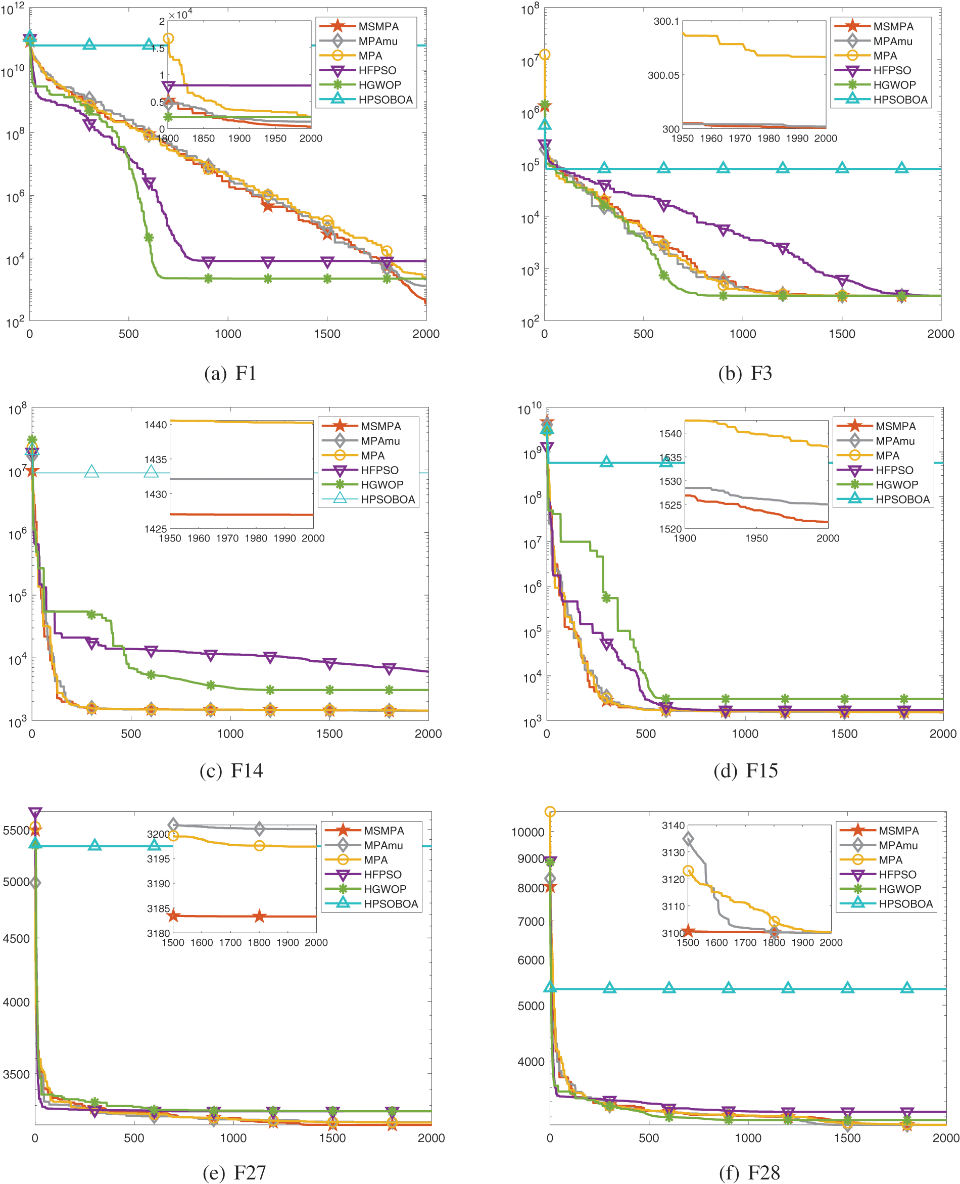
Figure 4: Convergence curves of algorithms on CEC2017 30D

In hybrid functions, MSMPA is particularly effective in finding the best results for F14 and F15. The second ranking among the ten functions reaches five times. In the Figs. 4c and 4d, not only the convergence speed but also the computational accuracy are well shown. It can be seen that MSMPA use the linear flight strategy and PSO search strategy, which is ahead of other algorithms in performance.

In the composition functions, the optimal average of functions F21, F22, F25, F26, F28 and F30 is represented by MSMPA, which obtains the most optimal values among all algorithms. In the computation of these functions, MPA performs better than MPAmu. This indicates that the multi-stage improvement mechanism of MSMPA as well as the self-adjusting weight work well for them. The connection between the pre-stage organisms is strengthened by the linear flight strategy, which increases the information transfer. The movement patterns of the later stage organisms are exploited by the PSO search mechanism, which is used to find the optimal prey.

In fact, MPA-related algorithms all have similar convergence curves. How to find a better convergence curve in the similarity is the direction of improvement in this paper. As can be seen from the table, MSMPA has significantly better computational accuracy for the three metaheuristics HFPSO, HGWOP and HPSOBOA. Likewise, it is excellent in the comparison with the two MPAs. It indicates that the population diversity is improved after using the linear flight strategy and self-adjusting weight. However, in the convergence graph, the convergence speed of MSMPA is not significant and only slightly faster than that of MPAs. This means that MSMPA has improved the convergence speed and population diversity compared with the comparison algorithms, but its convergence could still be improved in the future.

5  Structural Design Optimization Problems

5.1 Problem Description

In this section, the algorithm in this paper focuses on the analysis of three engineering optimization problems. Of course problems have been solved by other algorithms as well, so we can compare and analyze the practical applications of MSMPA. To eliminate randomness and variability, we choose the conventional 20∗D to bring into the problem and perform 30 independent trials. The D is the dimension, and then we calculate the obtained best value, worst value, optimal mean, standard deviation, and median, respectively. The termination condition of the gear train design for engineering optimization problem is set to a maximum number of 1000 iterations or a relative error of 10E−6.

5.2 Design of Pressure Vessel

The design problem of pressure vessel was first introduced by Kannan et al. [30]. The main shape of a pressure vessel is a cylindrical vessel which is capped at both ends by a hemispherical shaped head as shown in Fig. 5. It has a working pressure of 2000psi and a maximum volume of 750ft3. The main objective of the problem is to minimize the manufacturing cost of the pressure vessel, which mainly includes the cost of material, forming and welding. Four main variables are included: the thickness of the pressure vessel (Ts), thickness of the head (Th), inner radius of the vessel (R) and length of the vessel without heads (L). The first two variables are integer multiples of 0.0625. Separately, let the four variables be x1,x2,x3,x4. This equation is shown as Eq. (17).

Minimizef(X)=0.6224x1x3x4+1.7781x2x32+3.1661x12x4+19.84x12x3s.t.g1(X)=−x1+0.0193x3≤0g2(X)=−x2+0.0095x3≤0g3(X)=−πx32x4−43πx33+1296000≤0g4(X)=x4−240≤01×0.0625≤x1,x2≤99×0.0625;10≤x3,x4≤200(17)

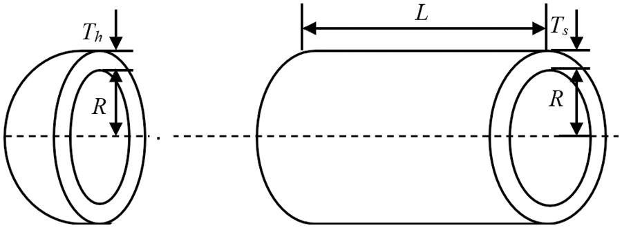
Figure 5: Pressure vessel structure diagram

There are also many algorithms that solve the problem, such as [24,25,29]. In Table 5, the objective function value of MSMPA is 5884.27383, which is much better than that of the comparison algorithms. In the Table 6, the optimal solution corresponding to the objective function value of each algorithm is listed, and the optimal solution of MSMPA is X=[0.8066,0.3971,41.7911,180.4828], which does not exceed the range of the constraints.

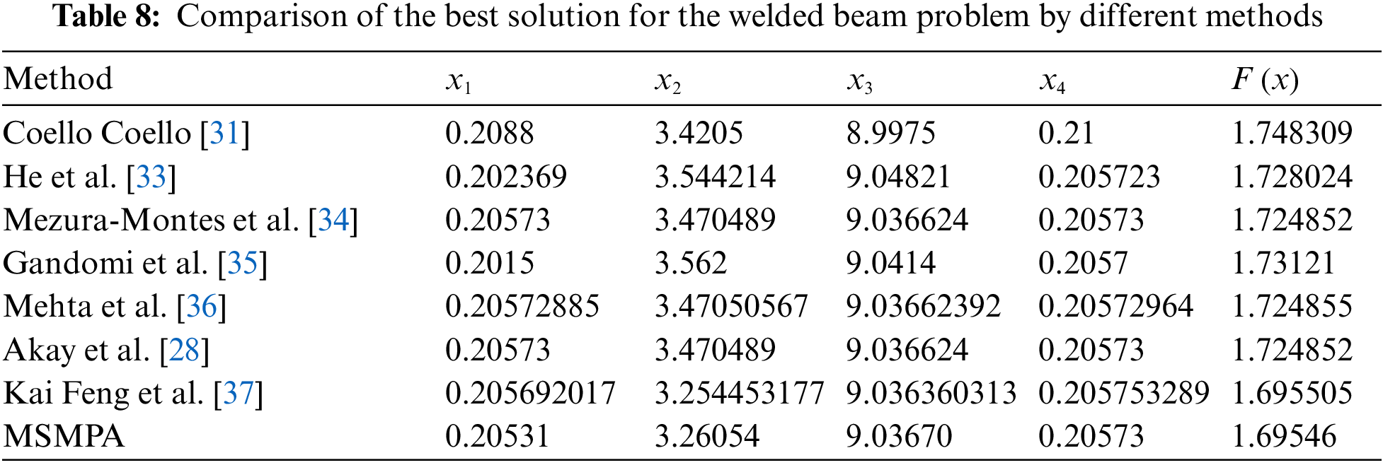
5.3 Welded Beam Design Problem

The welded beam design optimization problem is a commonly used engineering optimization problem with the structure shown in Fig. 6. It was first proposed by Coello Coello [31] in order to find the minimum manufacturing cost of welded beams. This cost problem is mainly influenced by the constraints of shear stress (τ), bending stress in the beam (θ), buckling load on the rod (PC), deflection at the beam end (δ) and lateral restraint. There are four optimization variables, which mainly include: weld thickness (h), connection beam length (l), beam height (t) and beam thickness (b). The mathematical model of the welded beam design problem is shown below:

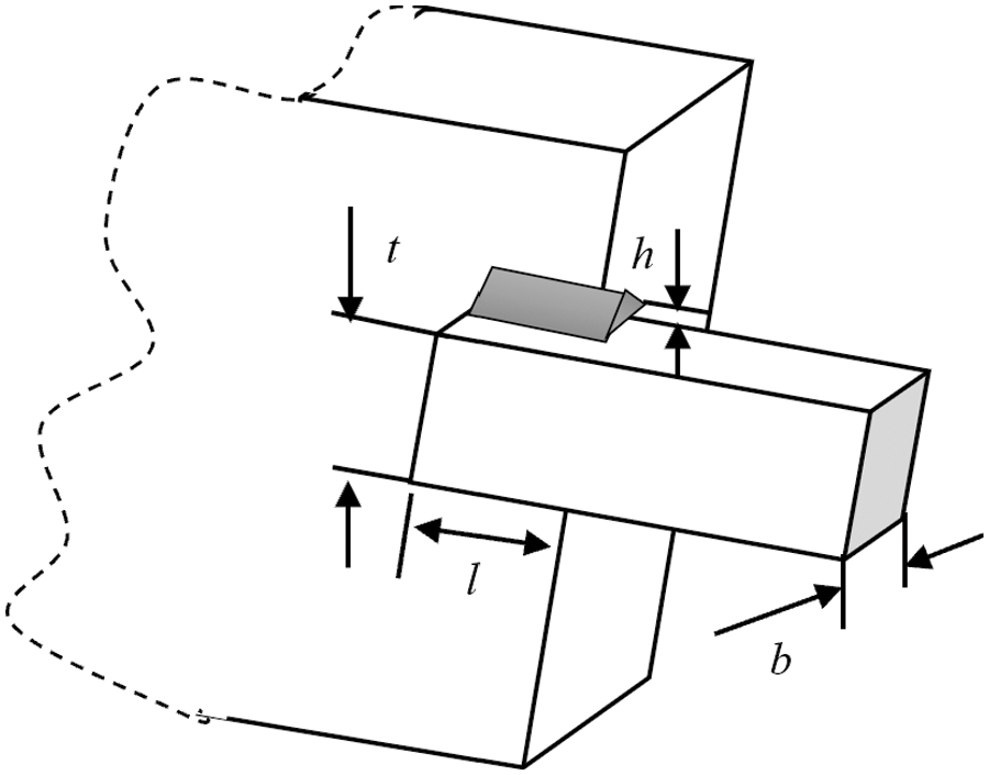
Figure 6: Welded beam structure diagram

Minimizef(X)=1.10471x12x2+0.04811x3x4(14+x2)s.t.g1(X)=τ(X)−τmax≤0g2(X)=θ(X)−θmax≤0g3(X)=x1−x4≤0g4(X)=0.125−x1≤0g5(X)=δ(X)−0.25≤0g6(X)=P−PC(X)≤0g7(X)=0.10471x12+0.04811x3x4(14+x2)−5≤00.1≤x1≤2;0.1≤x2≤10;0.1≤x3≤10;0.1≤x4≤2(18)

where x1,x2,x3,x4 correspond to four variables, τmax is the maximum allowable shear stress in the weld =13600psi, δmax is the maximum allowable bending stress in the beam =30000psi, and P=6000 lb is the load. The two components of the shear stress are the principal stress τ1 and the secondary stress τ2.

τ(X)=τ12+2τ1τ2(x22R)+τ22τ1=P2x1x2;τ2=MRJ(19)

where

M=P(L+x22);J(X)=2{2x1x2[x224+(x1+x32)2]}(20)

M and J(X) are known as moments and polar moment of inertia, respectively.

R=x224+(x1+x32)2;θ(X)=6PLx4x32;P=6000lbδ(X)=6PL3Ex33x4;PC(X)=4.013Ex32x4636L2(1−x32LE4G)G=12×106psi,E=30×106psi,L=14in(21)

The calculation results of different algorithms for this problem are shown in Table 7. The table shows that the best objective function value of MSMPA is 1.6954599, whose optimization ability is greatly improved. The optimal solutions of all algorithms are organized in Table 8. The optimal solution corresponding to the value of the objective function of MSMPA is X=[0.20531,3.26054,9.03670,0.20573] within the corresponding constraint.

5.4 Gear Train Design

The gear train design problem was first presented by Sandgren [24] as an unconstrained optimization problem. The problem is solved by minimizing the gear ratio cost of the gear train. The four decision variables defining the gear ratio are X=(Td,Tb,Ta,Tf)=(x1,x2,x3,x4) and the mathematical model of the problem is

Minimizef(X)=(16.931−x1x2x3x4)212≤x1,x2,x3,x4≤60;xi′s∈Z+(22)

The solutions of the problem by MSMPA algorithm and other algorithms are shown in Tables 9 and 10. The table shows that the accuracy of the MSMPA algorithm is higher than the other algorithms, and the objective function value, variance and standard deviation are smaller than the other algorithms. A linear flight strategy in the middle term and a strong development strategy in the middle and late term escort MSMPA to find the optimal gear ratio cost of the gear train. The optimal solution obtained by MSMPA is X=[12.7940,19.1888,60,28.3595], and the corresponding objective function value is 6.4396e−15.

6  Conclusions

Marine predators algorithm is a new algorithm proposed in 2020 and applied to many fields. Since MPA, like other intelligent algorithms, suffers from unbalanced exploration and exploitation, we improve it. In this paper, we proposed a new multi-stage improvement of marine predators algorithm. Firstly, the original Brownian motion is still used in the first stage, and the predation space is well expanded up. In the middle stage, the linear motion, which is more conducive to communication between creatures, is used to facilitate the fast movement of creatures far away from the prey. In the middle and late stages, the search mechanism of PSO is adopted, which effectively increases the exploitation ability of the creatures. At the same time, the constant P was changed to self-adjusting weight, thereby adapting more to the whole algorithmic process. The proposed MSMPA has been fully evaluated on CEC2017 functions and compared with established related optimization The experimental results show that MSMPA achieves competitive or even better performance on most functions, especially on composition. Also, in the engineering optimization problem, MSMPA has better objective function values compared to other algorithms and the resulting optimal solutions do not exceed the constraints. This indicates that the MSMPA algorithm can be well applied to engineering optimization problems.

In the future, we will continue to improve the algorithm and increase its performance. As the analysis of the experiment, we found that the convergence speed of MSMPA can still be improved and we can continue to experiment in this area at a later time. In addition, the predators model is a general optimization framework that can be applied to other metaheuristic algorithms, such as differential evolution (DE), genetic algorithm (GA), and artificial bee colony algorithm (ABC).

Funding Statement: This work was supported in part by National Natural Science Foundation of China (No. 62066001), Natural Science Foundation of Ningxia Province (No. 2021AAC03230) and Program of Graduate Innovation Research of North Minzu University (No. YCX22111). The authors would like to thank the anonymous reviewers for their valuable comments and suggestions.

Author Contributions: Chuandong Qin: Supervision, Validation, Project administration, Funding acquisition. Baole Han: Writing: original draft, Conceptualization, Methodology, Software. Writing: Review and editing, Methodology, Software, Data curation.

Ethics Approval: This paper does not contain any studies with human participants or animals performed by any of the authors.

Conflicts of Interest: The authors declare that they have no conflicts of interest to report regarding the present study.

References

1. Houssein, E. H., Gad, A. G., Hussain, K., Suganthan, P. N. (2021). Major advances in particle swarm optimization: Theory, analysis, and application. Swarm and Evolutionary Computation, 63(11), 100868. https://doi.org/10.1016/j.swevo.2021.100868 [Google Scholar] [CrossRef]

2. Golberg, D. E. (1989). Genetic algorithm in search, optimization, and machine learning. New York: Addison-Wesley Professional. [Google Scholar]

3. Kennedy, J., Eberhart, R. (1995). Particle swarm optimization. Proceedings of ICNN’95–International Conference on Neural Networks, pp. 1942–1948. Perth, Australia. [Google Scholar]

4. Sm, A., Smm, B., Al, A. (2014). Grey wolf optimizer. Advances in Engineering Software, 69, 46–61. [Google Scholar]

5. Zhang, C., Zhang, F. M, Li, F., Wu, H. S (2014). Improved artificial fish swarm algorithm. 2014 9th IEEE Conference on Industrial Electronics and Applications, Hangzhou, China. https://doi.org/10.1109/ICIEA.2014.6931262 [Google Scholar] [CrossRef]

6. Karaboga, D., Basturk, B. (2007). A powerful and efficient algorithm for numerical function optimization: Artificial bee colony (ABC) algorithm. Journal of Global Optimization, 39(3), 459–471. https://doi.org/10.1007/s10898-007-9149-x [Google Scholar] [CrossRef]

7. Faramarzi, A., Heidarinejad, M., Mirjalili, S., Gandomi, A. H. (2020). Marine predators algorithm: A nature-inspired metaheuristic. Expert Systems with Applications, 152(4), 113377. https://doi.org/10.1016/j.eswa.2020.113377 [Google Scholar] [CrossRef]

8. Houssein, E. H., Ibrahim, I. E., Kharrich, M., Kamel, S. (2022). An improved marine predators algorithm for the optimal design of hybrid renewable energy systems. Engineering Applications of Artificial Intelligence: The International Journal of Intelligent Real-Time Automation, 110(3), 104722. https://doi.org/10.1016/j.engappai.2022.104722 [Google Scholar] [CrossRef]

9. Al-Qaness, M., Ewees, A. A., Fan, H., Abualigah, L., Elaziz, M. A. (2022). Boosted ANFIS model using augmented marine predator algorithm with mutation operators for wind power forecasting. Applied Energy, 314(6), 118851.1–118851.12. https://doi.org/10.1016/j.apenergy.2022.118851 [Google Scholar] [CrossRef]

10. Sowmya, R., Sankaranarayanan, V. (2022). Optimal vehicle-to-grid and grid-to-vehicle scheduling strategy with uncertainty management using improved marine predator algorithm. Computers and Electrical Engineering, 100(2), 107949. https://doi.org/10.1016/j.compeleceng.2022.107949 [Google Scholar] [CrossRef]

11. Fan, Q., Huang, H., Chen, Q., Yao, L., Huang, D. (2022). A modified self-adaptive marine predators algorithm: Framework and engineering applications. Engineering with Computers, 38(4), 3269–3294. https://doi.org/10.1007/s00366-021-01319-5 [Google Scholar] [CrossRef]

12. Elaziz, M. A., Mohammadi, D., Oliva, D., Salimifard, K. (2021). Quantum marine predators algorithm for addressing multilevel image segmentation. Applied Soft Computing, 110, 107598. https://doi.org/10.1016/j.asoc.2021.107598 [Google Scholar] [CrossRef]

13. Han, M., Du, Z., Zhu, H., Li, Y., Yuan, Q. et al. (2022). Golden-sine dynamic marine predator algorithm for addressing engineering design optimization. Expert Systems with Applications, 210(3), 118460. https://doi.org/10.1016/j.eswa.2022.118460 [Google Scholar] [CrossRef]

14. Hu, G., Zhu, X., Wang, X., Wei, G. (2022). Multi-strategy boosted marine predators algorithm for optimizing approximate developable surface. Knowledge-Based Systems, 254(3), 109615. https://doi.org/10.1016/j.knosys.2022.109615 [Google Scholar] [CrossRef]

15. Abdel-Basset, M., Mohamed, R., Abouhawwash, M. (2022). Hybrid marine predators algorithm for image segmentation: Analysis and validations. Artificial Intelligence Review, 55, 3315–3367. https://doi.org/10.1007/s10462-021-10086-0 [Google Scholar] [CrossRef]

16. Kamaruzaman, A. F., Zain, A. M., Yusuf, S. M., Udin, A. (2013). Levy flight algorithm for optimization problems—A literature review. Applied Mechanics and Materials, 421, 496–501. https://doi.org/10.4028/www.scientific.net/AMM.421.496 [Google Scholar] [CrossRef]

17. Reynolds, A. M., Frye, M. A. (2007). Free-flight odor tracking in Drosophila is consistent with an optimal intermittent scale-free search. PLoS One, 2(4), e354. [Google Scholar] [PubMed]

18. Sims, D. W., Southall, E. J., Humphries, N. E., Hays, G. C., Bradshaw, C. J. et al. (2008). Scaling laws of marine predator search behaviour. Nature, 451(7182), 1098–1102. [Google Scholar] [PubMed]

19. Humphries, N. E., Queiroz, N., Dyer, J. R., Pade, N. G., Musyl, M. K. et al. (2010). Environmental context explains Lévy and Brownian movement patterns of marine predators. Nature, 465(7301), 1066–1069. [Google Scholar] [PubMed]

20. Faramarzi, A., Heidarinejad, M., Mirjalili, S., Gandomi, A. H. (2020). Marine predators algorithm: A nature-inspired metaheuristic. Expert Systems with Applications, 152, 113377. [Google Scholar]

21. Aydilek, Ä. B. (2018). A hybrid firefly and particle swarm optimization algorithm for computationally expensive numerical problems. Applied Soft Computing Journal, 66(2), 232–249. [Google Scholar]

22. Zhang, X., Lin, Q., Mao, W., Liu, S., Liu, G. (2021). Hybrid particle swarm and grey wolf optimizer and its application to clustering optimization. Applied Soft Computing, 101(9), 107061. https://doi.org/10.1016/j.asoc.2020.107061 [Google Scholar] [CrossRef]

23. Zhang, M., Long, D., Qin, T., Yang, J. (2020). A chaotic hybrid butterfly optimization algorithm with particle swarm optimization for high-dimensional optimization problems. Symmetry, 12(11), 1–27. https://doi.org/10.3390/sym12111800 [Google Scholar] [CrossRef]

24. Sandgren, E. (1988). Nonlinear integer and discrete programming in mechanical design. International Design Engineering Technical Conferences and Computers and Information in Engineering Conference, vol. 26584. Kissimmee, Florida, USA, American Society of Mechanical Engineers. [Google Scholar]

25. Gandomi, A. H., Yang, X. S., Alavi, A. H. (2013). Cuckoo search algorithm: A metaheuristic approach to solve structural optimization problems. Engineering with Computers, 29(1), 17–35. https://doi.org/10.1007/s00366-011-0241-y [Google Scholar] [CrossRef]

26. Coello Coello, C. A., Dhaenens, C., Jourdan, L. (2010). Multi-objective combinatorial optimization: Problematic and context. Studies in Computational Intelligence, 272, 1–21. https://doi.org/10.1007/978-3-642-11218-8 [Google Scholar] [CrossRef]

27. He, S., Prempain, E., Wu, Q. H. (2004). An improved particle swarm optimizer for mechanical design optimization problems. Engineering Optimization, 36(5), 585–605. https://doi.org/10.1080/03052150410001704854 [Google Scholar] [CrossRef]

28. Akay, B., Karaboga, D. (2012). Artificial bee colony algorithm for large-scale problems and engineering design optimization. Journal of Intelligent Manufacturing, 23(4), 1001–1014. https://doi.org/10.1007/s10845-010-0393-4 [Google Scholar] [CrossRef]

29. Hassanien, A. E., Rizk-Allah, R. M., Elhoseny, M. (2018). A hybrid crow search algorithm based on rough searching scheme for solving engineering optimization problems. Journal of Ambient Intelligence and Humanized Computing, 119(4), 1–25. https://doi.org/10.1007/s12652-018-0924-y [Google Scholar] [CrossRef]

30. Kannan, B. K., Kramer, S. N. (1994). An augmented lagrange multiplier based method for mixed integer discrete continuous optimization and its applications to mechanical design. Journal of Mechanical Design, Transactions of the ASME, 116(2), 405–411. https://doi.org/10.1115/1.2919393 [Google Scholar] [CrossRef]

31. Coello Coello, C. A. (2000). Use of a self-adaptive penalty approach for engineering optimization problems. Computers in Industry, 41(2), 113–127. https://doi.org/10.1016/S0166-3615(99)00046-9 [Google Scholar] [CrossRef]

32. Dimopoulos, G. G. (2007). Mixed-variable engineering optimization based on evolutionary and social metaphors. Computer Methods in Applied Mechanics and Engineering, 196(4–6), 803–817. https://doi.org/10.1016/j.cma.2006.06.010 [Google Scholar] [CrossRef]

33. He, Q., Wang, L. (2007). An effective co-evolutionary particle swarm optimization for constrained engineering design problems. Engineering Applications of Artificial Intelligence, 20(1), 89–99. https://doi.org/10.1016/j.engappai.2006.03.003 [Google Scholar] [CrossRef]

34. Mezura-Montes, E., Coello Coello, C., Velázquez-Reyes, J., Munoz-Dávila, L. (2007). Multiple trial vectors in differential evolution for engineering design. Engineering Optimization, 39(5), 567–589. https://doi.org/10.1080/03052150701364022 [Google Scholar] [CrossRef]

35. Gandomi, A. H., Yang, X. S., Alavi, A. H. (2011). Mixed variable structural optimization using firefly algorithm. Computers and Structures, 89(23–24), 2325–2336. https://doi.org/10.1016/j.compstruc.2011.08.002 [Google Scholar] [CrossRef]

36. Mehta, V. K., Dasgupta, B. (2012). A constrained optimization algorithm based on the simplex search method. Engineering Optimization, 44(5), 537–550. https://doi.org/10.1080/0305215X.2011.598520 [Google Scholar] [CrossRef]

37. Feng, Z. K., Niu, W. J., Liu, S. (2021). Cooperation search algorithm: A novel metaheuristic evolutionary intelligence algorithm for numerical optimization and engineering optimization problems. Applied Soft Computing, 98, 106734. https://doi.org/10.1016/j.asoc.2020.106734 [Google Scholar] [CrossRef]

38. Deb, K., Goyal, M. (1996). A combined genetic adaptive search (GeneAS) for engineering design. Computer Science and Informatics, 26, 30–45. [Google Scholar]

39. Garg, H. (2016). A hybrid PSO-GA algorithm for constrained optimization problems. Applied Mathematics and Computation, 274(5), 292–305. https://doi.org/10.1016/j.amc.2015.11.001 [Google Scholar] [CrossRef]