
 Submit a Paper
 Propose a Special lssue
 Open Access
ARTICLE

An Enhanced Adaptive Differential Evolution Approach for Constrained Optimization Problems
College of Mechanical Engineering, Zhejiang University of Technology, Hangzhou, 310023, China
* Corresponding Author: Zhi Pei. Email:
(This article belongs to the Special Issue: Computing Methods for Industrial Artificial Intelligence)
Computer Modeling in Engineering & Sciences 2023, 136(3), 2841-2860. https://doi.org/10.32604/cmes.2023.027055
Received 11 October 2022; Accepted 25 November 2022; Issue published 09 March 2023
 View Full Text
 Download PDF
Abstract
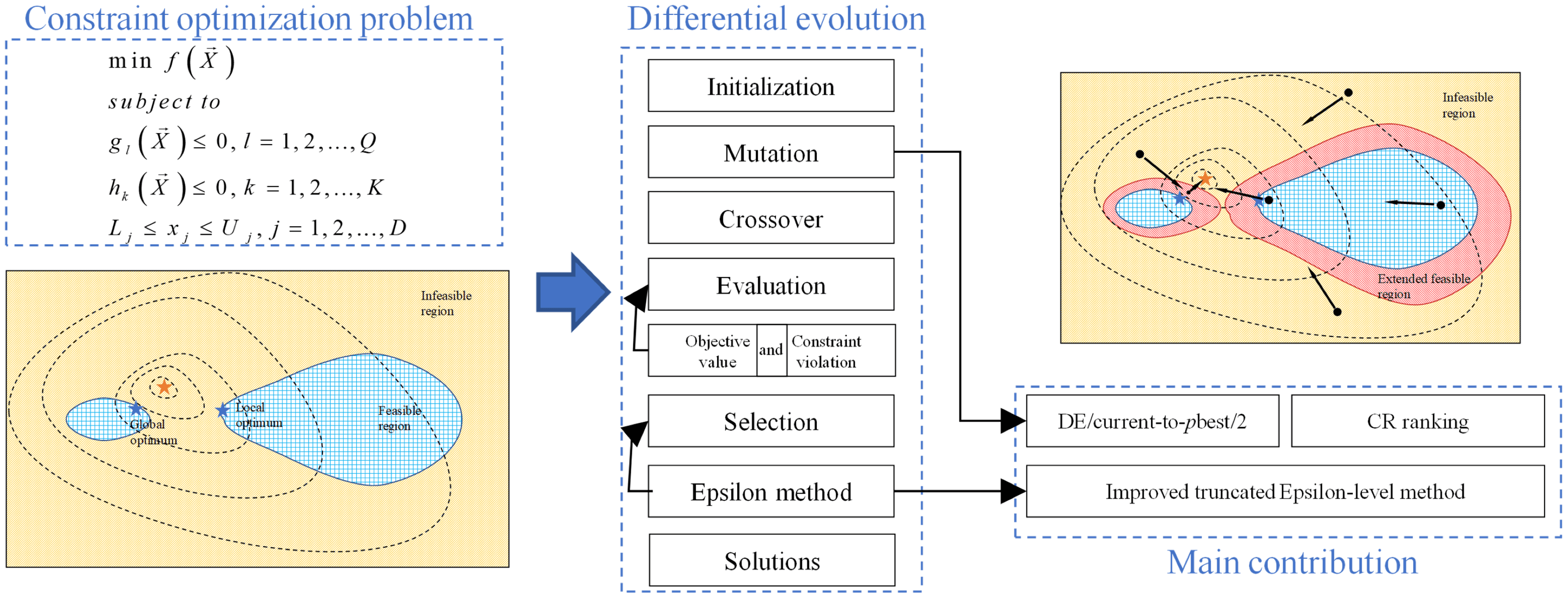
Effective constrained optimization algorithms have been proposed for engineering problems recently. It is common to consider constraint violation and optimization algorithm as two separate parts. In this study, a pbest selection mechanism is proposed to integrate the current mutation strategy in constrained optimization problems. Based on the improved pbest selection method, an adaptive differential evolution approach is proposed, which helps the population jump out of the infeasible region. If all the individuals are infeasible, the top 5% of infeasible individuals are selected. In addition, a modified truncated ε-level method is proposed to avoid trapping in infeasible regions. The proposed adaptive differential evolution approach with an improved ε constraint process mechanism (IεJADE) is examined on CEC 2006 and CEC 2010 constrained benchmark function series. Besides, a standard IEEE-30 bus test system is studied on the efficiency of the IεJADE. The numerical analysis verifies the IεJADE algorithm is effective in comparison with other effective algorithms.Graphic Abstract
Keywords
Numerous real-world engineering optimization problems, such as the milling process [1] and design problems of the car sides [2], are typical constrained optimization problems (COPs). A set of constraints and the objective function are needed to meet at the same time. The mathematical model can be presented in the following way:
where
In the literature, traditional mathematical programming-based approaches and computational intelligence algorithms are applied to tackle COPs. Traditional methods, such as the gradient-based approaches, often require a priori knowledge of the mathematical properties of the model. While computational intelligence methods do not rely on that a priori knowledge, but can still present more robust and better solutions than traditional methods.
Evolutionary algorithms, e.g., the differential evolution (DE) algorithm, are effective ways to deal with the COPs. DE algorithm is effectively used as the search engine. Since the first proposal of Storn et al. [3], many scholars have contributed continuously to improve it. Zhang et al. [4] introduced the adaptive DE algorithm, JADE, by proposing an effective mutation strategy and adaptive control parameter generation method. Gong et al. proposed a series of essential and effective improvements to JADE [5]. A strategy adaption mechanism and a crossover rate repairing technique are presented. The researches show that the improvements of JADE are competitive compared with other algorithms.
Combined with the constraint handling techniques, DE can be utilized in COPs [6–9]. The most effective ones are penalty function method [10], multi-objective-based method [11], ε constraint handling technique [12], stochastic ranking (SR) [13], and so on. As a classical constraint handling technique, penalty function method requires appropriate penalty parameters to get better results. The superiority of feasible solutions (SF) [14] is embedded in the selection phase, which gives priority to ensuring all solutions are feasible, and then optimizes the objective function values. However, promising infeasible solutions should be retained at the beginning of the iteration to help the population move to a better region. Fu et al. [9] proposed the hyperspace dynamic region to store infeasible solutions, which can improve the performance of the algorithm.
ε constraint handling technique is a promising method proposed nowadays, which accepts the promising constraint violation individuals at first, and then accepts those feasible solutions at the end of the evolution process. Takahama et al. [12] first introduced the ε constraint method into DE algorithm (εDE). The feasible solutions can be obtained quickly, and better objective values are achieved as well. Then they brought in a revised εDE via the kernel regression-based approximation [15]. Unfortunately, this method is time-consuming due to its approximation procedure. Wang et al. [16] integrated both SF and ε constraint handling technique into composite differential evolution. Its comprehensive performance is better than those using only one constraint handling method. Zhang et al. [17] presented an adaptive ε control heuristic method in place of using exponential function to control ε value. Stanovov et al. [18] integrated a selective pressure technique in DE, which takes function values, constraint violations measured by ε-constraint level into consideration simultaneously. Aiming to the multipath estimation in non-Gaussian noise problem, Ni et al. [19] integrated ε-constrained method into differential evolution. Duc Nguyen et al. [20] integrated differential evolution in Adaptive-Network-based Fuzzy Inference System. The experiment results prove the method is better than Reduced Error Pruning Trees and Decision Stump. Yi et al. [21] presented an improved version of ε-constrained method with adaptive differential evolution.
ε constraint method can adjust the feasible region adaptively in a more effective way. And the ε-level control method plays an important role in balancing exploration and exploitation. Hence, an improved version of ε constraint method is proposed in this paper.
The main purpose of the paper is to design an effective constraint technique and optimization algorithm for COPs. Therefore, the following two innovations are made:
1) First, the pbest selection mechanism is proposed. Rather than selecting the individuals with respect to the objective values, the individuals are chosen based on constraint violation and fitness.
2) Second, an improved ε constraint method is proposed. The reasonable setting of ε is important. Hence, a novel truncated setting is proposed to ensure that.
The framework of the paper can be summarized as below. Section 2 presented the proposed algorithm, with an improved top pbest individual selection mechanism in JADE for COPs. In Section 3, the improved ε constrained method is presented. In Section 4, the proposed algorithm is compared with several DE variants via benchmark testing problems. In Section 5, the standard IEEE‐30 bus test system is used to test the efficiency of the proposed algorithm. And Section 6 concludes the paper.
2 Adaptive Differential Evolution for COPs
An improved JADE that tackles the COPs is proposed. The pbest selection mechanism will be introduced.
2.1 DE/Current-to-pbest/2 Strategy
DE/current-to-pbest/2 strategy is:
where xr3, xr4 are two randomly selected individuals in population.
In JADE, the archive is used to collect unsuccessful solutions, and it can serve to improve the global search capability. The difference vector can point to the better area by archive set. The archive can be helpful in exploitation, which can also be harmful in investing unpromising areas. Emphasis on the exploration, the archive is not included in our paper. To give a vivid description on the proposed strategy, Function 8 with two-dimensional variables in CEC 2006 benchmark [22] is used as an example to illustrate our idea. The objective function, constraint violation and the mutation vector generation with the proposed strategy diagram are drawn as Figs. 1 and 2.
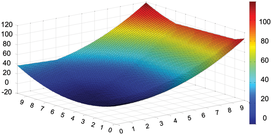
Figure 1: Constraint violation of F08 in CEC 2006
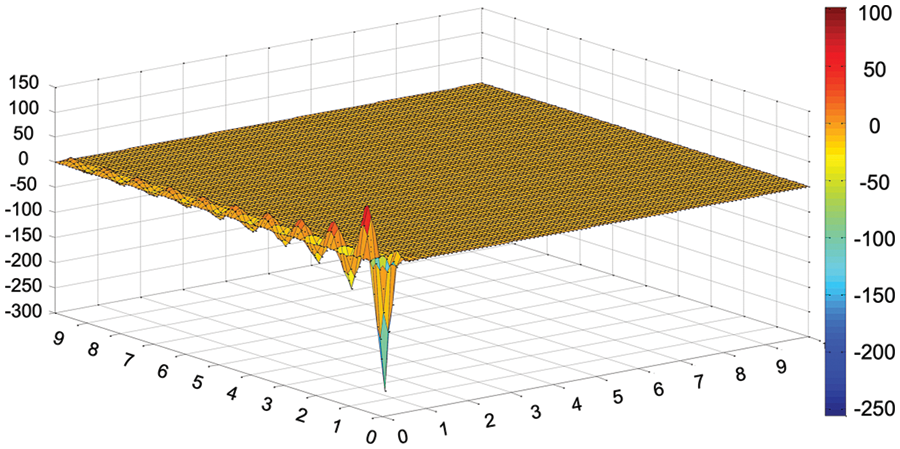
Figure 2: Objective function value of F08 in CEC 2006
We can see from Fig. 3, the proposed strategy can guide the target vector moving towards the promising area, and moving away from the more constraint violation area. In this way, more exploration can be made within the promising area.
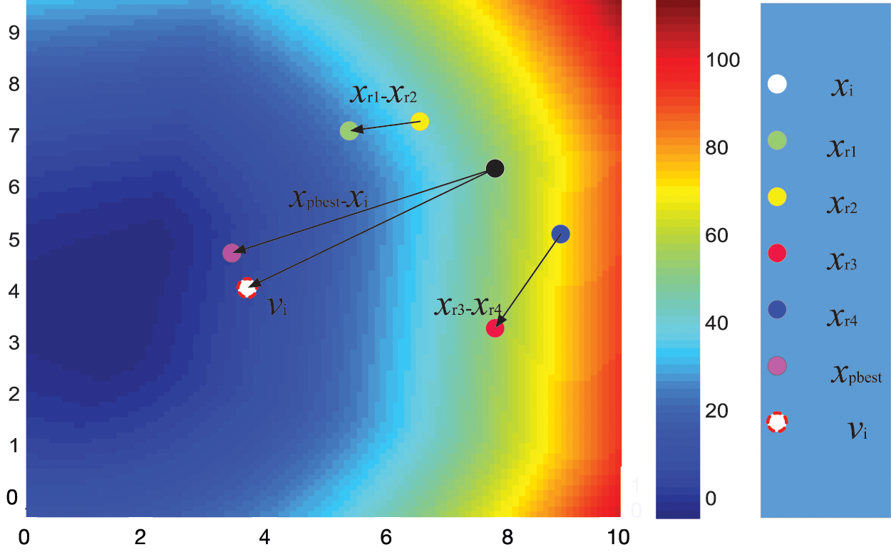
Figure 3: Illustration of the proposed strategy in F08
2.2 Parameter Adaption Strategy
Control parameters Fi and CRi are from various distribution and mean values. In this way, they can move towards the promising areas.
The CRi generation in JADE [4] is given as:
where
The Fi is similar to CRi generation with following formula:
where
Fitness and constraint violation are both vital in COPs. ε constrained algorithm is effective in dealing with the two indexes. The improved ε setting will be given in the following part.
In-line equations/expressions are embedded into the paragraphs of the text. For example,
Constraint violation
where
Based on the concept of constraint violation, COPs can be presented as follows:
In usual comparison strategy, x is defined as feasible when
where
ε-level setting is vital in ε constrained method [21,23]. Above researches show that ε should be larger at first and decrease along with constraint violation.
Static ε control method was firstly proposed [12] and it uses exponent function control the decrease of ε-level:
where
Truncated ε-level method uses the maximum and minimum constraint violation in the population to calculate ε-level:
where
Using static ε control method, the ε-level is related to the initial constraint violation during the generation, excluding current information of population. If the initial violation value is too large, it will slow down the convergence speed and lean to be stuck in the local optimum within the infeasible region. Although the truncated ε-level method exploits the information of the present population, for complicate equality constraints, the strategy may lead the population trapping into the infeasible region.
In this paper, an improved ε-level setting is presented as follows:
A proper setting of
A revised truncated strategy is implemented.
Fitness value and feasibility are both vital in COPs. Feasibility often is more important than fitness value. A selection strategy for pbest individuals with respect to the constraint violation is presented. If two individuals are both infeasible, the one with less constraint violation is better. If they are both feasible, their objective function values are compared instead.
Based on the above analysis, the pseudocode of the proposed algorithm is shown in Fig. 4.
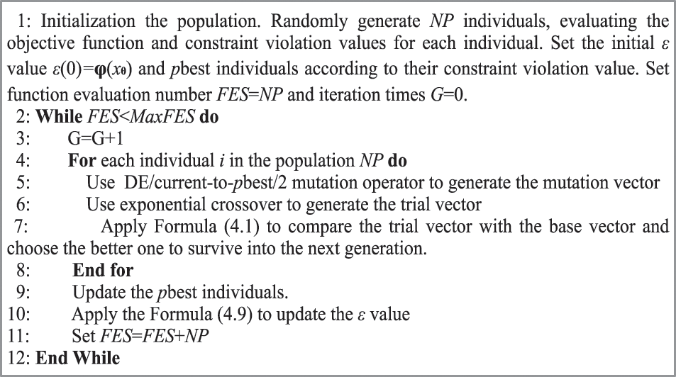
Figure 4: Pseudocode of the proposed improved adaptive differential evolution with modified ε constrained method
To examine the performance quantitatively, two benchmark function sets are used: CEC 2006 and CEC 2010, where D = 10, 30 are analyzed. For simplicity’s sake, the detailed forms of the test functions are omitted. The details can be referred in Liang et al. [22] and Mallipeddi et al. [24], respectively.
It is worth mentioning that the CEC 2010 benchmark functions with 10D have twelve functions which feasible region ratio less than 10E−06, and thirteen functions with 30D benchmark functions. Referring to the feasible region ratio, it is more difficult to solve the CEC 2010 benchmark functions than CEC 2006 series.
For the proposed algorithm, the parameters are set as below:
• population size: 80 (CEC 2006), 20 (10D, CEC 2010), 50 (30D, CEC 2010);
• crossover rate:
• scaling factor:
• ε setting control parameter:
• maximum number of fitness evaluations: 500,000; D * 20,000 (CEC 2010);
where
Three state-of-the-art algorithms APF-GA [25], Cultural CPSO [26] and AIS [27] are used as the baselines to measure the performance of the proposed IεJADE method. Since all the three algorithms cannot guarantee feasibility for functions G20 and G22, the comparisons on these two benchmark functions are omitted. The experimental results of APF-GA, Cultural CPSO and AIS are from Zhang et al. [23].
We can conclude from Table 1, the APF-GA method converges to the most desirable results in 16 functions, which are G01, G03-04, G06-09, G11-14, G16, G18 and G24 in terms of the “Best” and “Mean” indexes. The Cultural PSO algorithm can attain the best outcome in 17 out of 22 functions, which are G01, G03-12, G14, G16, G18, G21 and G23-24 referring to the “Best” and “Mean” indexes. 7 out of 20 functions can obtain the most desirable results for AIS algorithm with respect to the “Best” and “Mean” indexes, which are G01, G08, G11-12, G15-16 and G19. The proposed IεJADE algorithm secure the best solution in 13 out of 22 functions, which are G02, G04-G14 and G16. The proposed IεJADE algorithm rivals the APF-GA and Cultural-CPSO algorithm, and outperforms the AIS algorithm with respect to the overall performance. In particular, APF-GA algorithm attains the best outcome in G05 and G10 in terms of the “Best” index without a tie. Similarly, Cultural-PSO reaches the best results in G02 and G03, AIS in G02, G04-05, G07, G09-10, G14, G18, G21 and G23, IεJADE in G03, G15, G17-18, G21 and G23. As for the “Best” index, the IεJADE algorithm shows superior performance than APF-GA and Cultural-CPSO algorithms. To sum up, the proposed IεJADE is an effective algorithm in solving the CEC 2006 benchmark functions.

For comprehensive comparison, AIS and εDEg are chosen to compare with IεJADE. εDEg [28] is ranked first in the competition at CEC 2010, while the AIS algorithm is recently proved to be effective for COPs. And the best outcome of all the three algorithms is written in bold. The experimental results of CEC 2010 on 10D and 30D are given in Tables 2 and 3, respectively.


In contrast with the two other algorithms in 10D problems, the proposed IεJADE algorithm obtains the best results of index “Best” in 9 out of 18 functions, which are C01-02, C04, C07-10, C14 and C18. As for the “Median”, “Mean” and “Worst” indexes, the proposed IεJADE algorithm obtains best outcome in 10, 6, and 6 out of 18 functions, respectively. AIS attains the best result in 10, 5, 6, and 6 out of 18 functions, as for the indexes of “Best”, “Median”, “Mean” and “Worst”. The εDEg algorithm achieves 11, 9, 9, 9 out of 18 functions referring to “Best”, “Median”, “Mean” and “Worst” indexes. In summary, the εDEg approach outperforms the other algorithms in 10D problems.
Compared with two competitive algorithms in 30D problems, the proposed IεJADE algorithm attains the best results in terms of “Best”, “Median”, “Mean”, and “Worst” in 11, 13, 8, and 7 out of 18 functions. The AIS algorithm reaches 6, 5, 4, and 5 best results out of 18 functions in the above indexes. εDEg algorithm obtains 1, 1, 5, and 5 best results in the “Best”, “Median”, “Mean”, and “Worst” indexes, respectively. It is worth mentioning that the proposed IεJADE algorithm demonstrates superior capabilities in handling the 30D problems, in comparison with the other two algorithms.
To conclude, the proposed algorithm has potential in solving complex and high dimensional problems while the performance in low dimensional problems is acceptable when compared with the two competitive algorithms.
4.4 Convergence Curve of ε-Level
The convergence curves of the 10 functions with 30 dimensions are given as follows. From Fig. 5, it is observed that the IεJADE algorithm can achieve convergence with a rapid speed. The convergence curves of ε-level also indicate that the proposed setting can be convergent to the original feasible region rapidly with a small number of fitness evaluations.
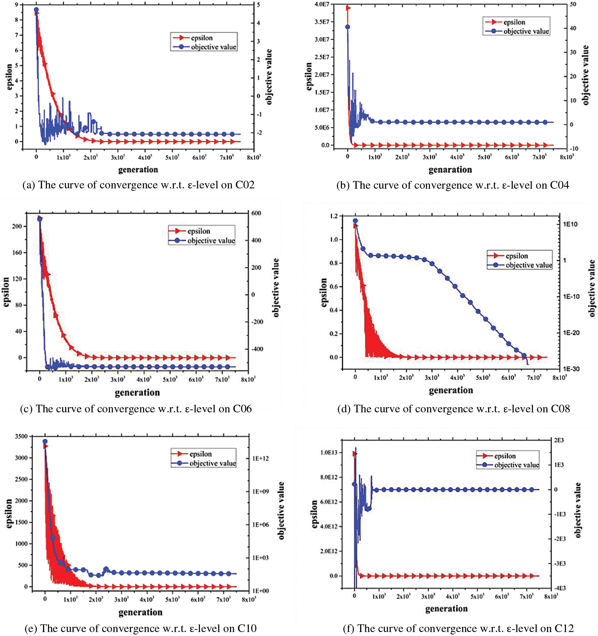
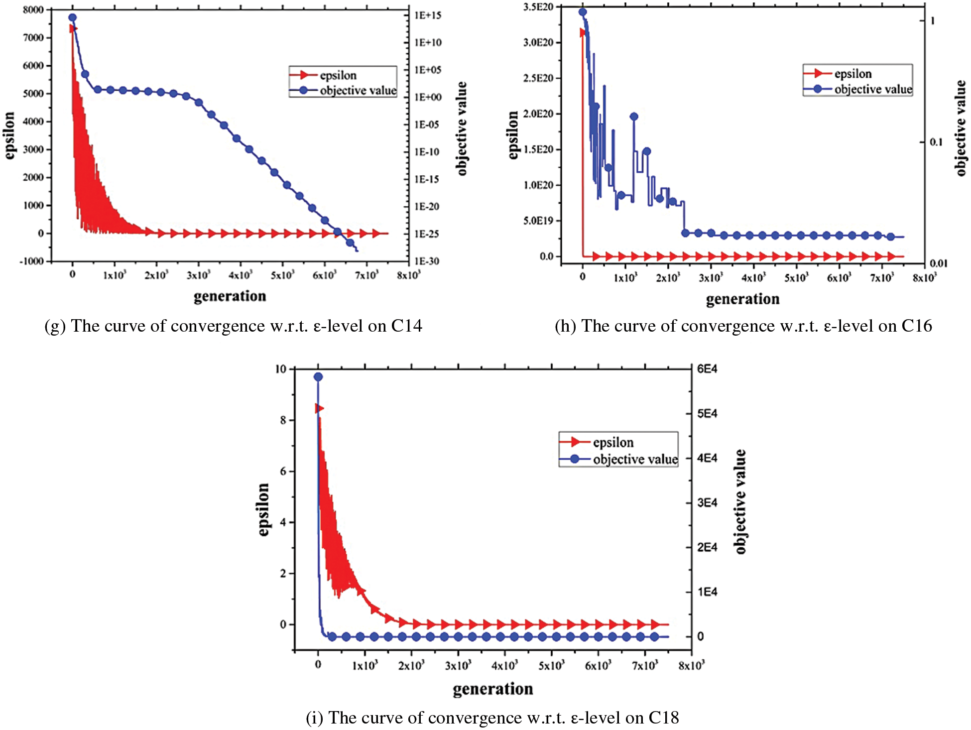
Figure 5: The curve of convergence w.r.t. ε-level
A standard IEEE-30 bus test system is utilized to evaluate the effectiveness of the IεJADE algorithm. As one of the leading cases in power systems optimization, optimal power flow (OPF) aims to obtain the optimal solutions and minimize the objective function. Equality and inequality constraints are two different optimal objectives in this system, which are described in following subsection.
In OPF, typical load flow equations can be illustrated as follows:
where
The inequality constraints are as follows:
where
Two single optimal objectives, minimization of emission and minimization of real power loss are studied. Emission in traditional electrical power system have been concerned as it emits harmful gases including SOx, NOx. The equation of minimization of emission is given by [29]:
where

The power loss is unavoidable but it can be reduced by adjusting voltage and voltage angle. The equation of real power loss is expressed as:
The standard IEEE-30 bus system is used and four optimization objectives, including fuel cost, emission, fuel cost with valve-point effect and voltage deviation are considered. The ACDE [29], ECHT-DE [30], SF-DE [30], and SP-DE [30] are compared with the proposed approach. The results are given in Table 5.

The best results are in bold. It can be concluded that the proposed IεJADE algorithm has competitiveness in this application. In Case 1, the proposed algorithm can obtain the best results as other state-of-the-art algorithms. In Case 2, the proposed algorithm can achieve the best Max, Mean and Std values, which means IεJADE has the most stable performance than other algorithms.
In the IEEE 30-bus system, the load bus voltage has its limits [0.95−1.05 p.u.] [29]. Fig. 6 shows the load bus voltages are within the permissible range.
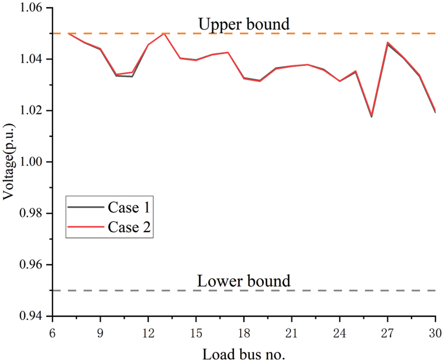
Figure 6: The voltage of load bus by IεJADE
To effectively tackle the constraints in COPs, an improved pbest selection mechanism and an adaptive ε setting are presented. The effectiveness of the proposed algorithm is tested on benchmark test functions in CEC 2006, CEC 2010, and the standard IEEE 30-bus test system. The numerical results illustrate that the proposed IεJADE algorithm is effective in tackling the constrained benchmark test functions and real-world applications. The proposed pbest selection mechanism presents a way to select and compare the infeasible and feasible individuals, which is effective to tackle them as integrity rather than two separate parts.
The improved pbest selection mechanism focus on finding feasible solution first. Therefore, it is more suitable for solving problems with smaller feasible domains. If a feasible solution can be easily found, the pbest strategy which directly optimizes the objective function is more suitable.
It is challenging to obtain suitable ε values. The proposed ε setting can be improved by machine learning and other self-learning ways. Historical information can be used to obtain the values. IεJADE algorithm can be used to tackle more complex engineering-based constrained optimization problems [31–33] in the future. Besides, more optimal objectives in IEEE 30-bus test system can be considered in further research.
Funding Statement: This research was supported by National Natural Science Foundation of China under Grant Nos. 52005447, 72271222, 71371170, 71871203, L1924063, Zhejiang Provincial Natural Science Foundation of China under Grant No. LQ21E050014, and Foundation of Zhejiang Education Committee under Grant No. Y201840056.
Conflicts of Interest: The authors declare that they have no conflicts of interest to report regarding the present study.
References
1. Sönmez, A. İ., Baykasoǧlu, A., Dereli, T., Fılız, İ. H. (1999). Dynamic optimization of multipass milling operations via geometric programming. International Journal of Machine Tools and Manufacture, 39(2), 297–320. https://doi.org/10.1016/S0890-6955(98)00027-3 [Google Scholar] [CrossRef]
2. Gu, L., Yang, R. J., Tho, C., Makowskit, M., Faruquet, O. et al. (2001). Optimisation and robustness for crashworthiness of side impact. International Journal of Vehicle Design, 26(4), 348. https://doi.org/10.1504/IJVD.2001.005210 [Google Scholar] [CrossRef]
3. Storn, R., Price, K. (1997). Differential evolution−A simple and efficient heuristic for global optimization over continuous spaces. Journal of Global Optimization, 11(4), 341–359. https://doi.org/10.1023/A:1008202821328 [Google Scholar] [CrossRef]
4. Zhang, J., Sanderson, A. C. (2009). JADE: Adaptive differential evolution with optional external archive. IEEE Transactions on Evolutionary Computation, 13(5), 945–958. https://doi.org/10.1109/TEVC.2009.2014613 [Google Scholar] [CrossRef]
5. Gong, W., Cai, Z., Wang, Y. (2014). Repairing the crossover rate in adaptive differential evolution. Applied Soft Computing, 15(4), 149–168. https://doi.org/10.1016/j.asoc.2013.11.005 [Google Scholar] [CrossRef]
6. Segundo, G. A. S., Krohling, R. A., Cosme, R. C. (2012). A differential evolution approach for solving constrained min-max optimization problems. Expert Systems with Applications, 39(18), 13440–13450. https://doi.org/10.1016/j.eswa.2012.05.059 [Google Scholar] [CrossRef]
7. Xu, B., Tao, L., Chen, X., Cheng, W. (2019). Adaptive differential evolution with multi-population-based mutation operators for constrained optimization. Soft Computing, 23(10), 3423–3447. https://doi.org/10.1007/s00500-017-3001-0 [Google Scholar] [CrossRef]
8. Nguyen, T. H., Vu, A. T. (2023). An efficient differential evolution for truss sizing optimization using adaboost classifier. Computer Modeling in Engineering & Sciences, 134(1), 429–458. https://doi.org/10.32604/cmes.2022.020819 [Google Scholar] [CrossRef]
9. Fu, L., Ouyang, H., Zhang, C., Li, S., Mohamed, A. W. (2022). A constrained cooperative adaptive multi-population differential evolutionary algorithm for economic load dispatch problems. Applied Soft Computing, 121(2), 108719. https://doi.org/10.1016/j.asoc.2022.108719 [Google Scholar] [CrossRef]
10. Gong, W., Cai, Z., Liang, D. (2015). Adaptive ranking mutation operator based differential evolution for constrained optimization. IEEE Transactions on Cybernetics, 45(4), 716–727. https://doi.org/10.1109/TCYB.2014.2334692 [Google Scholar] [PubMed] [CrossRef]
11. Wang, Y., Yin, D. Q., Yang, S., Sun, G. (2019). Global and local surrogate-assisted differential evolution for expensive constrained optimization problems with inequality constraints. IEEE Transactions on Cybernetics, 49(5), 1642–1656. https://doi.org/10.1109/TCYB.2018.2809430 [Google Scholar] [PubMed] [CrossRef]
12. Takahama, T., Sakai, S. (2006). Constrained optimization by the ε constrained differential evolution with gradient-based mutation and feasible elites. 2006 IEEE International Conference on Evolutionary Computation, pp. 1–8. Vancouver, BC, Canada. [Google Scholar]
13. Runarsson, T. P., Yao, X. (2000). Stochastic ranking for constrained evolutionary optimization. IEEE Transactions on Evolutionary Computation, 4(3), 284–294. https://doi.org/10.1109/4235.873238 [Google Scholar] [CrossRef]
14. Deb, K. (2000). An efficient constraint handling method for genetic algorithms. Computer Methods in Applied Mechanics and Engineering, 186(2), 311–338. https://doi.org/10.1016/S0045-7825(99)00389-8 [Google Scholar] [CrossRef]
15. Takahama, T., Sakai, S. (2013). Efficient constrained optimization by the ε constrained differential evolution with rough approximation using kernel regression. 2013 IEEE Congress on Evolutionary Computation, pp. 1334–1341. [Google Scholar]
16. Wang, B. C., Li, H. X., Li, J. P., Wang, Y. (2019). Composite differential evolution for constrained evolutionary optimization. IEEE Transactions on Systems, Man, and Cybernetics: Systems, 49(7), 1482–1495. [Google Scholar]
17. Zhang, C., Qin, A. K., Shen, W., Gao, L., Tan, K. C. et al. (2022). ε-Constrained differential evolution using an adaptive ε-level control method. IEEE Transactions on Systems, Man, and Cybernetics: Systems, 52(2), 769–785. https://doi.org/10.1109/TSMC.2020.3010120 [Google Scholar] [CrossRef]
18. Stanovov, V., Akhmedova, S., Semenkin, E. (2019). Selective pressure in constrained differential evolution. Proceedings of the Genetic and Evolutionary Computation Conference Companion, pp. 83–84. Prague Czech Republic, ACM. [Google Scholar]
19. Ni, Z. H., Cheng, L., Zhang, C. M. (2019). ε Constrained multi-mutant rank-based differential evolution algorithm and its application in multipath repression. 2019 IEEE 15th International Conference on Control and Automation (ICCA), pp. 893–898. Edinburgh, UK. [Google Scholar]
20. Duc Nguyen, M., Nguyen Hai, H., Al-Ansari, N., Amiri, M., Ly, H. B. et al. (2022). Hybridization of differential evolution and adaptive-networkbased fuzzy inference system in estimation of compression coefficient of plastic clay soil. Computer Modeling in Engineering & Sciences, 130(1), 149–166. https://doi.org/10.32604/cmes.2022.017355 [Google Scholar] [CrossRef]
21. Yi, W., Gao, L., Pei, Z., Lu, J., Chen, Y. (2021). ε Constrained differential evolution using halfspace partition for optimization problems. Journal of Intelligent Manufacturing, 32(1), 157–178. https://doi.org/10.1007/s10845-020-01565-2 [Google Scholar] [CrossRef]
22. Liang, J. J., Runarsson, T. P., Mezura-Montes, E., Clerc, M., Suganthan, P. N. et al. (2006). Problem definitions and evaluation criteria for the CEC 2006 special session on constrained real-parameter optimization. https://cw.fel.cvut.cz/b181/_media/courses/a0m33eoa/cviceni/2006_problem_definitions_and_evaluation_criteria_for_the_cec_2006_special_session_on_constraint_real-parameter_optimization.pdf [Google Scholar]
23. Zhang, C., Lin, Q., Gao, L., Li, X. (2015). Backtracking search algorithm with three constraint handling methods for constrained optimization problems. Expert Systems with Applications, 42(21), 7831–7845. https://doi.org/10.1016/j.eswa.2015.05.050 [Google Scholar] [CrossRef]
24. Mallipeddi, R., Suganthan, P. N. (2010). Problem definitions and evaluation criteria for the CEC 2010 competition on constrained real-parameter optimization. http://www.al-roomi.org/multimedia/CEC_Database/CEC2010/RealParameterOptimization/CEC2010_RealParameterOptimization_TechnicalReport.pdf [Google Scholar]
25. Tessema, B., Yen, G. G. (2009). An adaptive penalty formulation for constrained evolutionary optimization. IEEE Transactions on Systems Man and Cybernetics–Part A: Systems and Humans, 39(3), 565–578. https://doi.org/10.1109/TSMCA.2009.2013333 [Google Scholar] [CrossRef]
26. Zavala, A. E. M., Aguirre, A. H., Diharce, E. R. V. (2009). Continuous constrained optimization with dynamic tolerance using the COPSO algorithm. In: Constraint-handling in evolutionary optimization, pp. 1–23. Berlin, Heidelberg: Springer. [Google Scholar]
27. Zhang, W., Yen, G. G., He, Z. (2014). Constrained optimization via artificial immune system. IEEE Transactions on Cybernetics, 44(2), 185–198. https://doi.org/10.1109/TCYB.2013.2250956 [Google Scholar] [PubMed] [CrossRef]
28. Takahama, T., Sakai, S. (2010). Constrained optimization by the ε constrained differential evolution with an archive and gradient-based mutation. IEEE Congress on Evolutionary Computation, pp. 1–9. [Google Scholar]
29. Li, S., Gong, W., Hu, C., Yan, X., Wang, L. et al. (2021). Adaptive constraint differential evolution for optimal power flow. Energy, 235(8), 121362. https://doi.org/10.1016/j.energy.2021.121362 [Google Scholar] [CrossRef]
30. Biswas, P. P., Suganthan, P. N., Mallipeddi, R., Amaratunga, G. A. J. (2018). Optimal power flow solutions using differential evolution algorithm integrated with effective constraint handling techniques. Engineering Applications of Artificial Intelligence, 68(1), 81–100. https://doi.org/10.1016/j.engappai.2017.10.019 [Google Scholar] [CrossRef]
31. Liu, Z. Z., Wang, Y., Wang, B. C. (2021). Indicator-based constrained multiobjective evolutionary algorithms. IEEE Transactions on Systems, Man, and Cybernetics: Systems, 51(9), 5414–5426. https://doi.org/10.1109/TSMC.2019.2954491 [Google Scholar] [CrossRef]
32. Wang, B. C., Li, H. X., Zhang, Q., Wang, Y. (2021). Decomposition-based multiobjective optimization for constrained evolutionary optimization. IEEE Transactions on Systems, Man, and Cybernetics: Systems, 51(1), 574–587. https://doi.org/10.1109/TSMC.2018.2876335 [Google Scholar] [CrossRef]
33. Wen, L., Gao, L., Li, X., Li, H. (2022). A new genetic algorithm based evolutionary neural architecture search for image classification. Swarm and Evolutionary Computation, 75(5), 101191. https://doi.org/10.1016/j.swevo.2022.101191 [Google Scholar] [CrossRef]
Cite This Article
 Copyright © 2023 The Author(s). Published by Tech Science Press.
This work is licensed under a Creative Commons Attribution 4.0 International License , which permits unrestricted use, distribution, and reproduction in any medium, provided the original work is properly cited.
 Downloads
 Citation Tools