Quantum-Inspired Equilibrium Optimizer for Linear Antenna Array

1  Introduction

With the booming development of wireless technology, communication technology is gradually transforming from 2G to 5G [1]. In the process of wireless communication technology development, the antenna plays a vital role. For long distance communication, it is necessary to reduce the waste of energy by optimizing the antenna array. In order to obtain the maximum antenna radiation energy for a specific signal receiving point, it is necessary to reduce the SLL in the direction of disinterest so that the radiation energy is concentrated [2]. The radiation intensity and directionality of a single element antenna are challenging to maintain stability, while the antenna array can achieve the purpose by combining multiple elements [3]. The antenna array can have a narrow beam form and minimum SLL interference by adjusting the excitation amplitude and spacing of each array element as well as the geometric layout [4]. Most problems in engineering and technology can be attributed to optimization problems, and the optimization of linear antenna arrays is no exception. How to obtain high intensity radiation in a specific direction and the maximum reduction of SLL is gradually becoming a hot topic of research [5]. Modern antenna array design relies heavily on electromagnetic simulation models, but electromagnetic simulation is computationally expensive due to electromagnetic mutual inductance and other factors. The traditional numerical optimization method uses gradient information to adjust the antenna array design, but under the current computing conditions, the time cost of this optimization process is unacceptably high. How to efficiently use physics-based mathematical models to speed up the design process of antenna arrays is an important background for research [6]. Therefore, it is a challenging task to select an efficient computational method for numerical optimization. With the development of optimization theory and computer technology, some meta-heuristic optimization algorithms began to appear and attract the attention of scholars.

Metaheuristic algorithms are mainly inspired by natural phenomena and can be broadly classified into four categories. Evolutionary algorithms inspired by Darwinian evolutionary theory, mainly include genetic algorithm (GA) [7], evolutionary strategies (ES) [8], differential evolutionary algorithm (DE) [9], evolutionary planning (EP) [10], etc. Algorithms inspired by the intelligent behavior of biological swarms mainly include the particle swarm algorithm (PSO) [11], artificial bee colony algorithm (ABC) [12], chameleon algorithm (CSA) [13], barnacle mating algorithm (BMO) [14], whale optimization algorithm (WOA) [15], slap swarm algorithm (SSA) [16], gray wolf optimizer (GWO) [17], slime mould algorithm (SMA) [18], etc. Algorithms inspired by physical and chemical laws, mainly include artificial electric field algorithm (AEFA) [19], equilibrium optimizer (EO) [20], simulated annealing algorithm (SA) [21], big bang-big crunch (BBBC) [22], lightning search algorithm (LSA) [23], heat transfer search (HTS) [24], etc. The algorithms inspired by simulated human behavior mainly include teaching-learning-based optimization algorithm (TLBO) [25], brain storming algorithm (BSO) [26], volleyball premier league algorithm (VPLA) [27], etc. It is known from the No Free Lunch Theorem that no single meta-heuristic algorithm can perform well on all problems [28]. Therefore, meta-heuristic algorithms and their improved versions are continuously proposed by scholars for different optimization problems. Similarly, finding a more efficient method for solving the optimization problem of linear antenna arrays is still a hot research topic.

In 2019, Afshin Faramaki et al. proposed a novel physics-based optimization algorithm inspired by the mass balance equation in a container called the equilibrium optimizer [20]. Since its proposed simple structure and fast computing speed has attracted the attention of many scholars. In [29], Abdel-Basset et al. proposed a linear reduction diversity technique and local minima elimination method for basic equilibrium optimizer and applied the proposed improved equilibrium optimizer algorithm to solar cells. In [30], Gupta et al. used Gaussian variation and reconstruction concepts to compensate for the shortcomings of the basic equilibrium optimizer and applied them to multilayer perceptions training. In [31], Gao et al. proposed a binary version of the equilibrium optimizer and applied it to the feature selection problem to analyze the optimal choice of the transfer function. In [32], Wunnava et al. proposed an adaptive equilibrium optimizer that implements adaptive decentralized decision making for search agents. The proposed algorithm is also applied to multilevel shareholding segmentation of image histograms. In [33], Abdul-hamied et al. proposed a population-based equilibrium optimizer for the hybrid grid optimization problem. The problem combines economic-technical and environmental requirements to minimize the cost of power generation in the power system. In [34], Fan et al. introduced elite reverse learning with novel population update rules for the imbalance between exploration and exploitation of the basic equilibrium optimizer. The modified equilibrium optimizer is then tested on a classical function problem to verify that it has a fast convergence speed and optimality search accuracy. In [35], Elsheikh et al. used an equilibrium optimizer to tune the parameters of a random vector functional link network and predicted the quality metrics of sheet cuttings. In [36], Yin et al. hybridized the equilibrium optimizer with the smile mould algorithm and added a stochastic difference variation operator to make the algorithm escape from local optima. Finally, the proposed method search capability was verified in nine engineering design problems. In [37], Tang et al. proposed an equilibrium optimizer algorithm mixing multiple swarm strategies and applied it to the path planning problem. In [38], Abdel-Basset et al. proposed a multi-objective variant of the equilibrium optimizer that uses an archiving mechanism to retain the optimal solution and uses a crowded distance approach to maintain the diversity of solutions.

From the above, it is clear that the equilibrium optimizer has been successfully applied in many fields, but the basic equilibrium optimizer algorithm still has some shortcomings. Due to the existence of average candidate solutions in the equilibrium pool, the algorithm has a strong exploitation capability, which leads the equilibrium optimizer to converge early and fall into a local optimum. To address the shortcomings of the basic equilibrium optimizer algorithm and inspired by quantum computing, a novel quantum equilibrium optimizer algorithm is proposed. The idea of quantum coding is introduced in QEO to improve the basic equilibrium optimizer, which improves the equilibrium optimizer’s population diversity. Second, the original equilibrium pooling strategy is improved and combined with a quantum rotation gate to help the algorithm jump out of local optima. In the quantum equilibrium optimizer, the equilibrium optimizer update formula is mainly responsible for the change of the quantum phase angle, and the change of the probability amplitude is realized by the incremental calculation of the quantum rotation gate strategy.

In order to verify the feasibility and effectiveness of the QEO, this paper solves the problem of maximum SLL reduction for linear antenna arrays using the proposed algorithm. Three sets of LAA with a different number of array elements were selected as test examples, and QEO was used to compare with six novel meta-heuristic algorithms. The experimental statistics show that QEO has the advantages of fast convergence and high search accuracy and robustness.

The main contributions of this paper can be summarized as follows:

1.   Inspired by quantum computing to improve the original equilibrium optimizer seeking capability, a quantum coded version of the equilibrium optimizer algorithm is proposed.

2.   Introducing the idea of quantum coding, each individual in QEO corresponds to two positions in the search space, and the quantum coding mechanism improves the diversity of the population.

3.   Performing the incremental phase angle calculations through the combination of quantum rotation gate strategy and quantum equilibrium pool, which effectively helps the algorithm to jump out of local optimum and avoid premature convergence.

4.   QEO is used for linear antenna array optimization to maximize the SLL reduction. Three sets of LAA with a different number of array elements are selected for testing and compared with six novel meta-heuristic algorithms.

This paper is organized as follows. Section 2 expedites improving and applying different meta-heuristic algorithms for LAA optimization problems. Section 3 defines the maximum SLL reduction problem and the mathematical model. Section 4 describes the basic equilibrium optimizer. Section 5 describes the quantum equilibrium optimizer in detail. Section 6 shows the experimental results and statistical analysis results. The conclusion of our work is given in Section 7.

2  Related Works

2.1 Antenna Array Optimization

This section describes other metaheuristic algorithms and their modifications for antenna array optimization problems. In [39], Panduro et al. used a genetic algorithm for the design of non-uniform circular arrays and obtained a large reduction of SLL. In [40], Khodier et al. used the particle swarm algorithm to synthesize the minimum side lobe level and compared it with other algorithms to verify the effectiveness of the particle swarm algorithm. In [41], Guney et al. used the honeybee algorithm to adjust the phase and amplitude of the array elements, and the effectiveness of the method was verified on a Chebyshev antenna model. In [42], Singh et al. used the Biogeography-based optimization algorithm to adjust the optimal excitation amplitude of the antenna array elements and effectively synthesized the antenna radiation map. In [43], Pappula et al. used a cat swarm optimization algorithm for the optimal array element location to suppress the SLL, which has applications in electromagnetic optimization. In [44], Singh et al. used the cuckoo optimization algorithm (COA) to optimize the linear and circular arrays, and the experimental results showed that COA has superior performance. In [45], Dib et al. used a symbiotic bio-search algorithm to synthesize the radiation map of symmetric antenna arrays and effectively obtained a radiation map with low interference. In [46], Saxena et al. introduced the gray wolf optimization algorithm into the field of electromagnetic and antenna optimization to optimize the excitation amplitude and array element position to achieve the minimum SLL optimization. In [47], Salgotra et al. proposed an extended version of the gray wolf optimizer (GWO-E) that utilizes multiple swarm partitioning and adversarial learning strategies to improve the performance of the algorithm. Experiments show that GWO-E obtains the largest SLL reduction in a non-uniform antenna array. In [48], Wu et al. used a spider monkey optimization algorithm to optimize the synthesized sparse line array in order to reduce the side level of the whole array. In [49], Sun et al. used the weed invasion algorithm for beam synthesis of LAA with circular antenna array (CAA) and obtained better synthesis characteristics in a real environment. In [50], Durmus et al. applied the equilibrium optimizer algorithm to symmetric LAA with non-uniform CAA for radiation map synthesis to achieve narrow half-power beam widths. In [51], Sharaqa et al. used a bio-geographic optimization algorithm (BBO) to optimize the maximum SLL reduction and validated the effectiveness of BBO in comparison with other well-known optimization methods. In [52], Das et al. determination of excitation amplitude and antenna array spacing to reduce SLL values using the moth flame optimization method. In [53], Subhashini et al. used the runner-root algorithm (RRA) for linear antenna array optimization and obtained good results. In [54], Almagboul et al. proposed to optimize the beamformer weights using an atomic search optimization algorithm to minimize the SLL value. In [55], Singh et al. proposed a novel algorithm by fusing a differential evolutionary algorithm with harmonic search to synthesize the loop antenna array to minimize the SLL. In [56], Vegesna et al. improved flower pollination algorithms for beam forming techniques with highly minimized SLL. In [57], Liang et al. introduced migration strategy and elite learning mechanism in Biogeography-based optimization algorithm and proposed a new method with an adaptive variation strategy. The proposed method is then tested on a classical function and used for the antenna array beam optimization problem. In summary, the antenna array optimization problem has gradually become a hot area of research. The linear antenna array is the most basic antenna geometric arrangement and the most practical geometric arrangement, but it still suffers from the defect of insufficient maximum SLL reduction. Finding a more effective method to solve the linear antenna array optimization problem is still a hot research topic.

2.2 Quantum-Inspired Metaheuristic Algorithm

The concept of “quantum” first appeared in the last century in the field of physics, and it is in quantum computers that quantum properties are fully exploited [58]. This concept has attracted the attention of many scholars and introduced quantum theory into meta-heuristic algorithms. In [59], Yu et al. introduced the idea of quantum rotating gate to encode the population for the defect that the basic dragonfly optimization algorithm easily falls into local optimum. In [60], Zhang et al. proposed a quantum-inspired satin bowerbird optimizer algorithm to encode populations based on the quantum bits of Bloch spheres. In [61], Deng et al. proposed an efficient DE algorithm for solving large-scale optimization problems by introducing quantum computing features and co-evolutionary ideas to improve DE for the shortcomings of differential evolutionary algorithms. In [62], Zhou et al. proposed a quantum wind-driven optimization algorithm for unmanned aerial vehicle path planning problems with quantum non-gates for variation. In [63], Coelho et al. proposed a mutation-based quantum particle swarm algorithm (QPSO) inspired by quantum mechanics to prevent premature convergence of the algorithm. In [64], Zou et al. introduced dynamic population optimization strategies in TLBO and used quantum learning strategies to maintain population diversity. In [65], Yu et al. introduced the quantum rotating gate strategy and the water cycle mechanism into the basic smile mould algorithm to compensate for the early convergence. In [66], Cui et al. proposed a quantum-inspired moth flame optimizer for clustering on the UCI benchmark dataset to test efficiency. In [67], Li et al. proposed a new quantum coded pathfinder optimization algorithm for parameter optimization problem in proton exchange membrane fuel cells (PEMFC). Some scholars combine quantum computing ideas with meta-heuristic algorithms in the field of antenna optimization. In [68], Ho et al. proposed an improved quantum particle swarm algorithm that escapes from local optima by introducing diversification and intensification phases, and applied it to the optimization problem of a 28-element LAA. In [69], Patidar et al. used the quantum particle swarm method to optimize a broadband frequency-invariant pattern. In [70], Gao et al. combined the TLBO algorithm with quantum theory, made the population evolve in a good direction through the method of quantum revolving gate, and finally applied it to linear array pattern synthesis. In [71], Liu et al. combined quantum computing ideas with genetic algorithms to optimize the maximum signal output power. In [72], Mikki et al. used quantum particle swarm optimization for linear array antenna synthesis problems. The above articles have successfully integrated quantum ideas and heuristic algorithms and applied to the field of antennas, but there are still shortcomings in maximizing the effect of reducing SLL. While reducing the SLL problem is not novel, more efficient methods are absolutely needed. Therefore, this paper combines the physics-based equilibrium optimizer algorithm with quantum ideas for the first time, and proposes an efficient quantum equilibrium optimizer for reducing the SLL value, and fully compares it with other methods to show the advantages of QEO.

3  Problem Description

In this section, the mathematical model of SLL reduction for a linear antenna array is presented. The optimization process starts from the initialization of the problem, and a suitable fitness function should be selected as the optimization objective for each optimization problem. The linear antenna array is shown in Fig. 1, which contains 2M array elements.

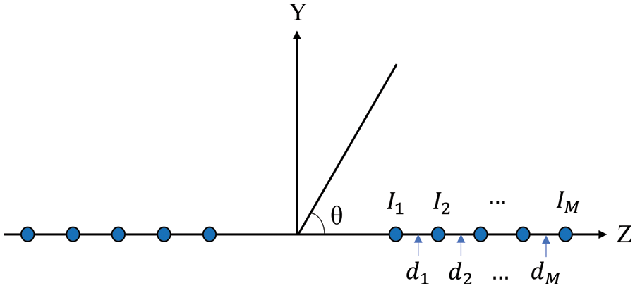
Figure 1: Linear antenna array with 2M elements

3.1 Antenna Factor

In a linear antenna array, all the elements are placed in a straight line. For the linear antenna, the array factor can be expressed as the combination of array excitation amplitude and position in array space. The linear antenna array element has the characteristics of uniform radiation pattern, but the array element excitation is concentrated in the center of the array when radiating together as an antenna array. The array factor can be expressed as follows [73]:

AF(φ)=2∑n=1MIncos⁡(kdcos⁡(φ)+ψn)(1)

where k=2π/λ is the wave number, In is excitation amplitude of elements, d represents the position of each element in the line array, ψn indicates the phase of each element, φ is the azimuth angle.

3.2 Fitness Function

In this paper, the excitation amplitude of the array elements in the linear antenna array is adjusted to make the antenna highly radioactivity in a specific direction. The optimization objective is to get the maximum SLL reduction and the fitness function can be expressed as:

fitness=max{20log10⁡|AF(φSL)||AF(φML)|}(2)

s.t. φML=arg⁡max|AF(φ)|,φ∈[0,π](3)

φSL∈[0,φFN1]∪[0,φFN2](4)

0<Ii<1,∀i∈M(5)

where φSL and φML are the interval between the values of the side lobe and the main lobe; φFN1 and φFN2 are the first nulls of the pattern; λ is wave length and array spacing fixed d=0.5λ; In order to ensure the maximum width of the first nulls of the pattern in the optimization process, φFN1 and φFN2 select the appropriate value.

4  Equilibrium Optimizer

The equilibrium optimizer [20] was first proposed to solve continuous optimization problems. The equilibrium optimizer has the advantages of strong computational stability and searching speed. The concentration update of the particle depends on the mass balance equation. The particle in the container (search agent) randomly updates its particle concentration until it reaches an equilibrium state (optimal result).

4.1 Inspiration

The equilibrium optimizer’s inspiration comes from the dynamic mass balance equation in the container for a control volume that describes the conservation of mass entering. The equation is defined as follows:

VdCdt=QCeq−QC+G(6)

where C is the concentration of particles, V is volume, Vdcdt is the rate of mass change, Q is the flow of volume,Ceq represents the equilibrium condition of particles, and G is the mass generation rate.

After obtaining the mass balance equation, the turnover rate (λ=QV) is introduced to rearrange the equation, and the solution time of the rearranged equation is solved as an integral of the function to obtain as follows:

C=Ceq+(C0−Ceq)F+GλV(1−F)(7)

where F is expressed as follows:

F=exp⁡[−λ(t−t0)](8)

where t0 and C0 is initiate time and start concentration.

4.2 Inspiration

As with most optimization methods, the searching flow path starts with initializing the container particle.

Cinitial=Cmin+rand(Cmax−Cmin)(9)

where Cinitial is the initial concentration of the particle, Cmin and Cmax are the maximum and minimum values of particle concentration, rand is a random number.

4.3 Equilibrium Pool

After that, the particle concentration is evaluated and four better fitness particles are chosen to constitute the equilibrium pool. The first four candidate solutions in the equilibrium pool are the particles with the best fitness values identified. However, and the last one of the equilibrium pool is the arithmetic mean of the four previous candidates as given in Eq. (10). Each iteration selects equilibrium candidate solutions with equal probability from the equilibrium pool.

C⟶avg=(C⟶eq(1)+C⟶eq(2)+C⟶eq(3)+C⟶eq(4))/4(10)

C⟶eq,pool={C⟶eq(1),C⟶eq(2),C⟶eq(3),C⟶eq(4),C⟶avg}(11)

where C⟶avg is the arithmetic mean, C⟶eq(1),C⟶eq(2),C⟶eq(3),C⟶eq(4) are the first four candidate solutions. C⟶eq,pool is an equilibrium pool.

4.4 Exponential Term

Exponential terms help enhance the exploration capabilities of the EO, and it is described as follows:

F⟶=a1sign(r⟶−0.5)[e−λ→t−1](12)

where a1 is a constant value, sign(r⟶−0.5) is a symbolic function in Eq. (12) has an effect on the searching direction, and time t is a nonlinear parameter. r⟶ and λ⟶ are a random vector between 0 and 1. It is calculated as follows:

t=(1−IterMax_iter)(a2IterMax_iter)(13)

where a2 is a constant value that controls exploitation capabilities, experiments show that when a1=2 and a2=1, EO has better optimization capability.

4.5 Generation Rate

The mass generation rate is helpful in improving the exploitation ability of the algorithm, and it is described as follows:

G⟶=G⟶0e−k⟶(t−t0)(14)

G⟶=G0⟶F⟶(15)

G0⟶=GCP→(Ceq⟶−λ⟶C⟶)(16)

GCP→={0.5r1,r2≥GP0,r2<GP(17)

where r1 and r2 are the random number, GCP is the generation rate control parameter.

The updating rule of EO is given as:

C⟶=C⟶eq+(C0⟶−Ceq⟶)F⟶+G⟶λ⟶V(1−F⟶)(18)

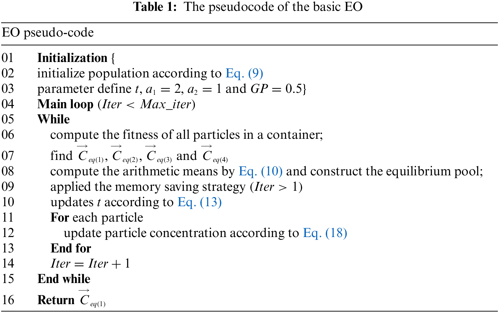
The first term in Eq. (18) selects a balanced candidate from the equilibrium pool. The existence of the equilibrium pool strategy enhances the exploration capability of the algorithm. The second is responsible for improving the global exploration capability of the algorithm, and the symbolic function controls different exploration directions. The third improves the exploitation capability of algorithms to control small changes in particle concentrations. The pseudocode of the basic EO is illustrated in Table 1.

4.6 Particle’s Memory Saving

This strategy is similar to the individual optimal location preservation strategy of PSO, which records the best location searched by individuals.

5  Quantum-Inspired Equilibrium Optimizer

In this section, a novel quantum meta-heuristic algorithm is proposed, the quantum equilibrium optimizer. QEO introduces the idea of quantum computing into the basic equilibrium optimizer, and uses the efficient computational performance of quantum computing to improve the optimization search capability of the basic equilibrium optimizer. After using quantum coding, a particle corresponds to two probability amplitude of quantum bits, it represents two positions in the optimization space, where the quantum probability amplitude is used to update the particle position and adjust the change of angle through the quantum rotation gate strategy. Inspired by quantum computing, a quantum equilibrium pooling strategy is proposed to realize the variation of quantum probability amplitude. The strategy improves the diversity of the population and avoids late premature convergence.

5.1 Quantum Computing and Chromosome Coding

The smallest unit in quantum computing is the quantum bit, which can be expressed as “0” and “1” for two states of quantum existence. A quantum bit can be expressed as follows:

|ψ⟩=α|0⟩+β|1⟩(19)

where α and β are the probability symbols of the quantum bits being 0 and 1, respectively; Due to the variable nature of the probability amplitude, it satisfies the equation |α|2+|β|2=1. The encoding of the individual quantum equilibrium optimizer inspired by the above quantum computing ideas is obtained as follows:

Xi=[α1α2…αDβ1β2⋯βD]=[cos⁡θ(i,1)cos⁡θ(i,2)…cos⁡θ(i,D)sin⁡θ(i,1)sin⁡θ(i,2)⋯sin⁡θ(i,D)](20)

where θ=2π×rand, rand is a random number between 0 and 1, i is the population size, D is the problem dimension.

Thus, quantum chromosomes correspond to two positions in quantum space, as follows:

Pic=(cos⁡θ(i,1),cos⁡θ(i,2),…,cos⁡θ(i,D))(21)

Pis=(sin⁡θ(i,1),sin⁡θ(i,2),…,sin⁡θ(i,D))(22)

5.2 Solution Space Transformation

In QEO, obtaining the particle positions corresponding to the problem requires mapping the quantum space of the quantum chromosome to the problem space σQEO=[a,b]. The quantum chromosome solution space transformation equation is as follows:

Xic=12[b(1+αi)+a(1−αi)](23)

Xis=12[b(1+βi)+a(1−βi)](24)

where Xic is the quantum state |0⟩ calculated by the probability amplitude αi, Xis is the quantum state |1⟩ calculated by the probability amplitude βi.

5.3 Updating Process

In order to improve the defect that the basic equilibrium optimizer algorithm tends to converge prematurely in the late iteration, this paper introduces a quantum rotation gate strategy with a quantum equilibrium pool strategy inspired by quantum computing. The angle variation of the quantum probability amplitude is adjusted by the quantum rotation gate, and the variation of the position is realized by the quantum equilibrium pool strategy.

5.3.1 Quantum Equilibrium Pool

We construct the quantum equilibrium pool for the phase angles of the quanta, calculate the phase angles of the four particles with the best adaptation values and save them in the quantum equilibrium pool. To improve the global exploration capability of the algorithm, the random phase angles θrand⟶ are randomly selected from the quantum population. The quantum equilibrium pool is constructed as follows:

θ⟶eq,pool={θ⟶eq1,θ⟶eq2,θ⟶eq3,θ⟶eq4,θ⟶rand}(25)

5.3.2 Updating Formulas of Phase Angle

In the quantum equilibrium optimizer, the phase angle update equation is as follows:

θi⟶(t+1)=θeq⟶+(θi⟶(t)−θeq⟶)×F⟶+G⟶λ⟶V(1−F⟶)(26)

where θeq⟶ denotes the randomly selected phase angle from the quantum equilibrium pool; θi denotes the phase angle of i-th particle in the quantum population.

5.3.3 Quantum Rotation Gate Strategy

In this section, the quantum rotation gate strategy is used to adjust the probability amplitude and to calculate the phase angle increment before adjusting the probability magnitude. To address the shortcomings of the basic equilibrium optimizer with insufficient convergence accuracy and exploration capability, the quantum equilibrium pool variation strategy is introduced to calculate the rotation gate increments. The combination of powerful computational power of quantum computing and optimization algorithm makes QEO the ability to escape the optimal local solution, which effectively improves the algorithm search accuracy.

Δθi⟶=(b−a)×rand⟶×(θrand⟶−θeq,pool⟶)(27)

where Δθi⟶ phase angle is increment, a and b are the lower and upper bounds of the problem space, respectively. rand⟶ Represents a random vector of 0 to 1, θeq,pool⟶ is the equilibrium candidate phase angle in the quantum equilibrium pool. The probability amplitude update equation through the quantum rotation gate is as follows:

[cos⁡(θi⟶(t+1))sin⁡(θi⟶(t+1))]=[cos⁡(Δθi⟶(t+1))−sin⁡(Δθi⟶(t+1))sin⁡(Δθi⟶(t+1))cos⁡(Δθi⟶(t+1))][cos⁡(θi⟶(t))sin⁡(θi⟶(t))]=[cos⁡(θi⟶(t+1)+Δθi⟶(t+1))sin⁡(θi⟶(t+1)+Δθi⟶(t+1))](28)

The corresponding quantum chromosome positions are as follows:

Pic⟶=(cos⁡(θ1(t+1)+Δθ1(t+1)),…,cos⁡(θj(t+1)+Δθj(t+1)))(29)

Pis⟶=(sin⁡(θ1(t+1)+Δθ1(t+1)),…,sin⁡(θj(t+1)+Δθj(t+1)))(30)

5.4 The Flow Chart and Pseudocode of QEO

In order to show the QEO algorithm more clearly, Table 2 and Fig. 2 respectively show the pseudocode and flow chart of the quantum equilibrium optimizer.

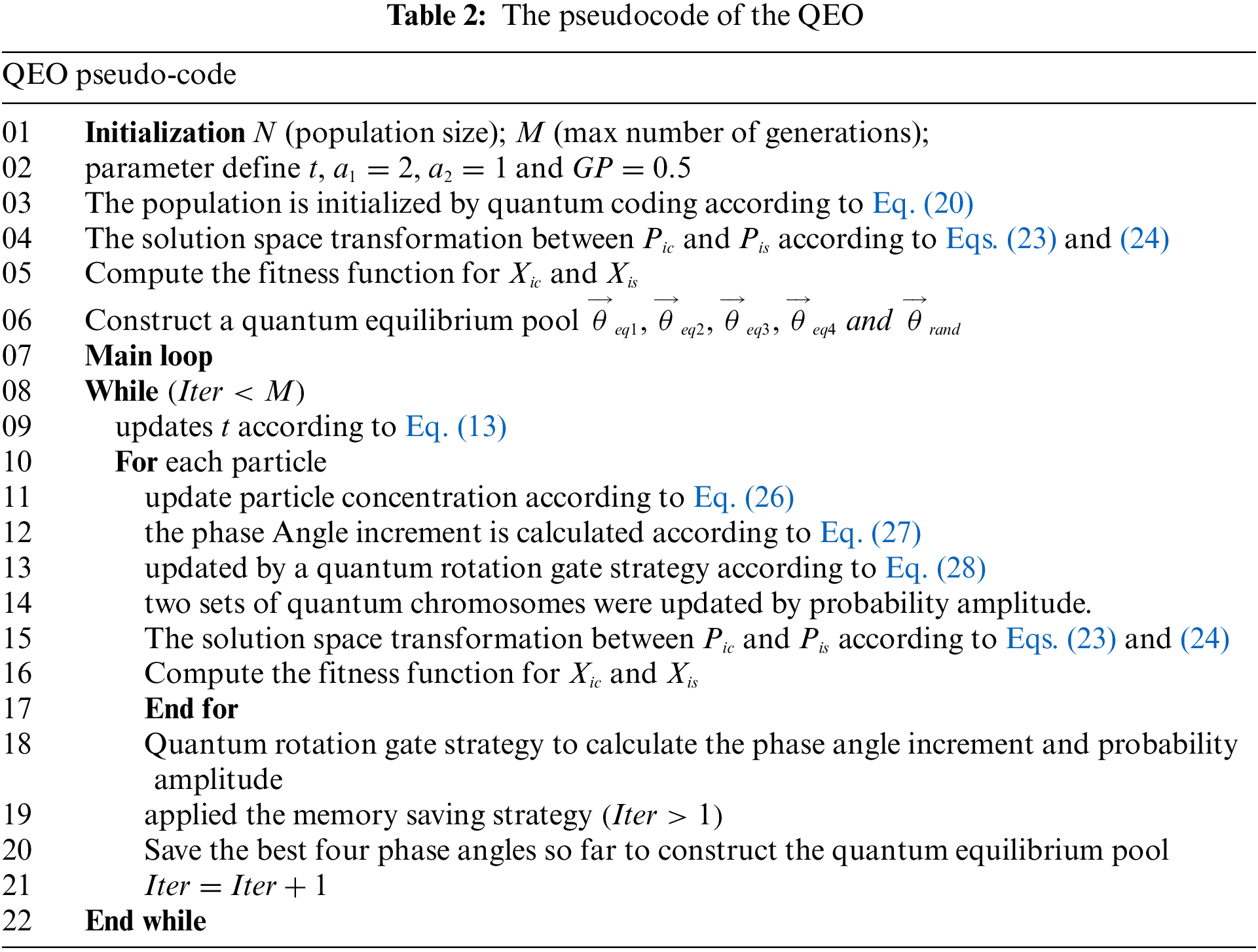
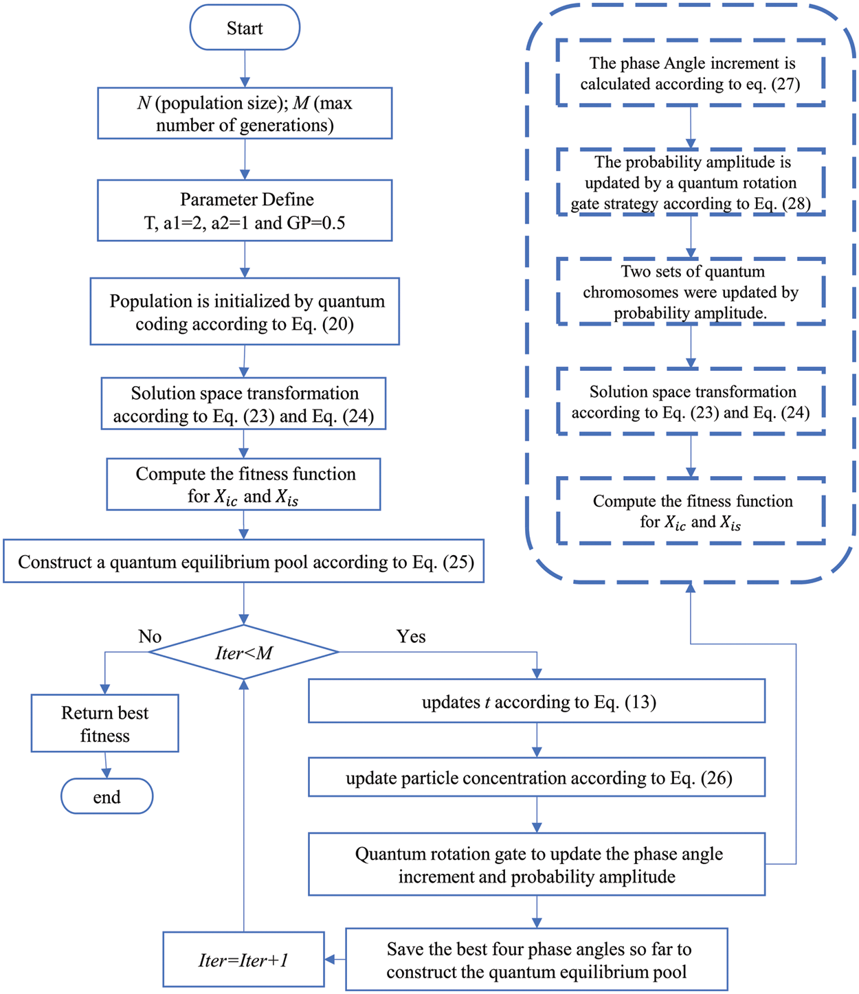
Figure 2: The flow chart of QEO

6  Experimental Results and Discussions

For validating the robustness and effectiveness of the proposed algorithm in solving the maximum SLL optimization problem, the QEO was tested on 16, 24 and 32 elements LAA. Our experiments application MATLAB 2019a and run-on CPU Intel Core i7-9700 processor 3.0 GHz, 16 GB RAM.

6.1 Performance Metrics

The performance of different comparison algorithms in the maximum SLL optimization problem was evaluated using the following measures:

•   Max and Min: Maximum values and minimum values in the calculation results of thirty independent runs.

•   Ave: The average value of the calculation results of thirty independent runs, which is calculated as follows:

Ave=1runs∑i=1runsFi(31)

•   STD: It is used to show the computational stability of the algorithm. The formula is as follows:

Std=1runs−1∑i=1runs(Fi−Ave)2(32)

•   Wilcoxon’s rank-sum: WRS is a nonparametric test that takes a p-value that controls acceptance or rejection of the alternative hypothesis.

6.2 Comparative Algorithms

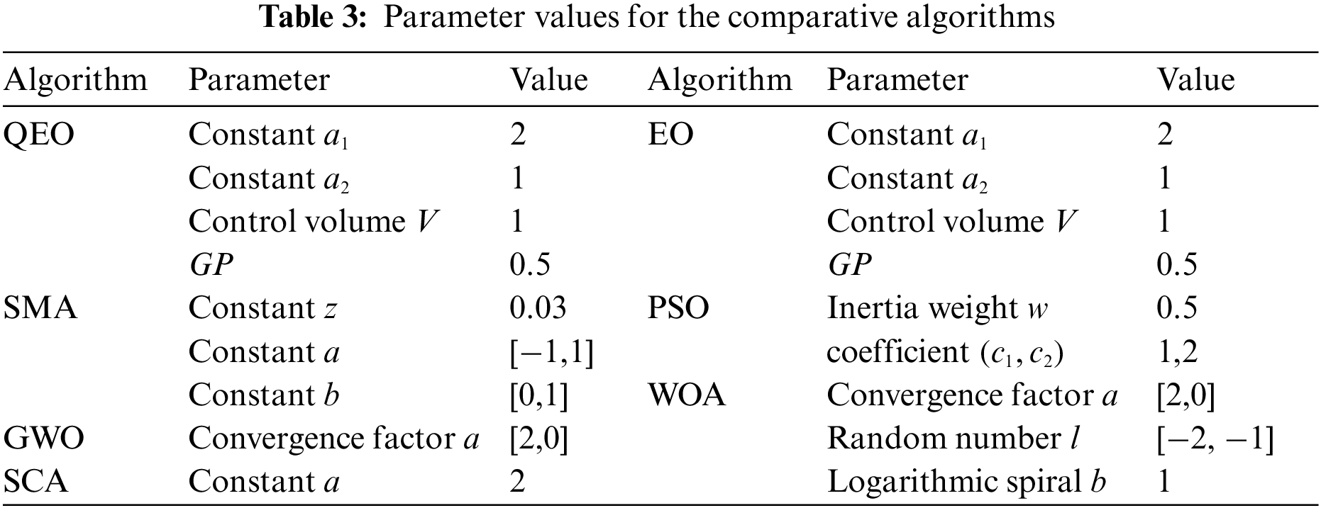
The experiment compared QEO with other novel algorithms, such as EO [20], SMA [18], PSO [11], SCA [74], WOA [15], GWO [17]. N is the population size and T is the maximum iterations. It is worth mentioning that the 16, 24 and 32 elements LAA, the population size is set to 30 and maximum iterations are set to 100. The parameter settings of the comparative algorithms in the experiment are shown in Table 3. The experimental parameter settings of the comparison algorithm are from its references. The experimental results come from all the algorithms running independently for 30 times under the same conditions, and the results were statistically analyzed.

6.3 Results and Discussion

In this section, we investigated the LAA optimization problem, namely verifying the effectiveness of the quantum equilibrium optimizer in reducing the SLL of LAA. QEO is tested with six other novel meta-heuristic algorithms in a linear array with different arrays of elements and four performance evaluation metrics are used to evaluate the optimization capability of the algorithms. The optimization results of different algorithms in the 16-element LAA with the excitation amplitude can be seen in Table 4. QEO obtains the optimal SLL value is −29.6939 dB, while the conventional method obtains the SLL is −13.1529 dB, and QEO improves 16.5410 dB compared to the conventional method. And the maximum SLL obtained by EO, SMA, PSO, SCA, WOA, and GWO is −28.4299, −28.3060, −23.7392, −25.6562, −28.7441, and −28.5342 dB. Beam patterns after optimization of the excitation amplitude by different algorithms are shown in Fig. 3. It can be seen that the QEO SLL is the smallest and the main beam has good radiation capability. The optimization results of different algorithms in 24-element LAA are shown in Table 5. Compared to the conventional values without optimization, the maximum SLL of QEO, EO, SMA, PSO, SCA, WOA, and GWO is reduced by 16.49, 14.75, 13.56, 8.12, 9.37, 12.59, and 13.71 dB, respectively. Compared to the conventional method, QEO showed the largest reduction. The QEO-optimized beam patterns partials beam is lower and the main beam has the best radiation intensity compared to other algorithms as seen in Fig. 4. As seen in Table 6 in the 32-element LAA, the maximum SLL obtained by QEO is significantly better than the other algorithms. As seen in Fig. 5, the optimized beam patterns of the proposed method are significantly better than other algorithms waveform levels are more distinct. As the number of LAA elements increases, QEO is able to adapt well to the computational difficulties associated with the increased problem size and obtains a larger SLL reduction compared to other algorithms. Figs. 6–8 show the three-dimensional antenna patterns of different array elements obtained by different optimization algorithms. From the figure, it can be observed that the QEO obtains the smallest side lobe level.

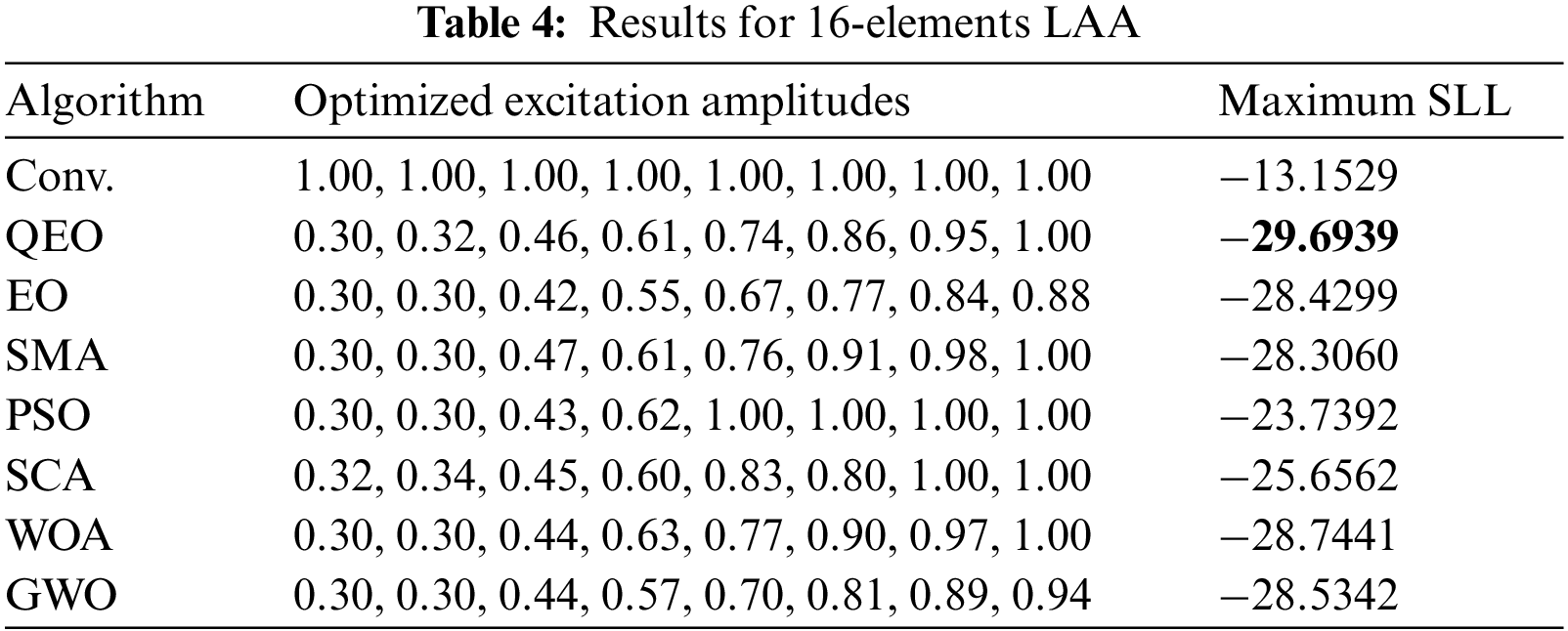
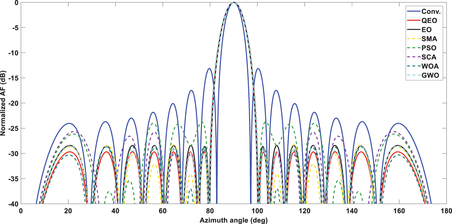
Figure 3: 2D beam patterns for 16-elements LAA

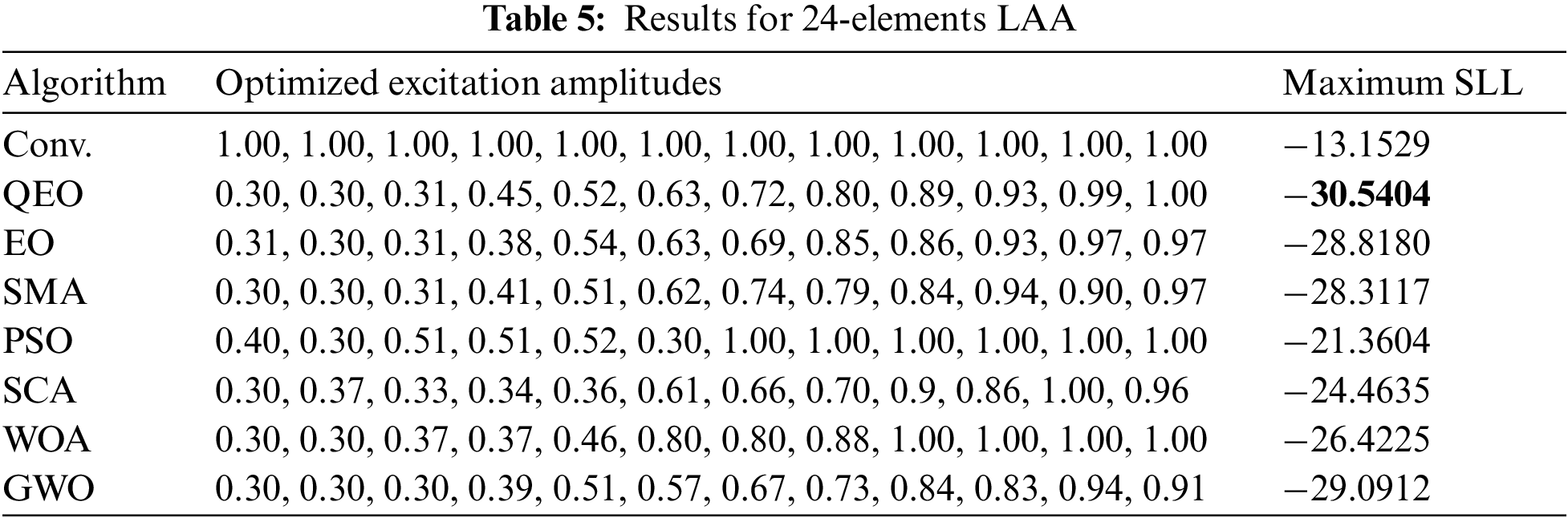
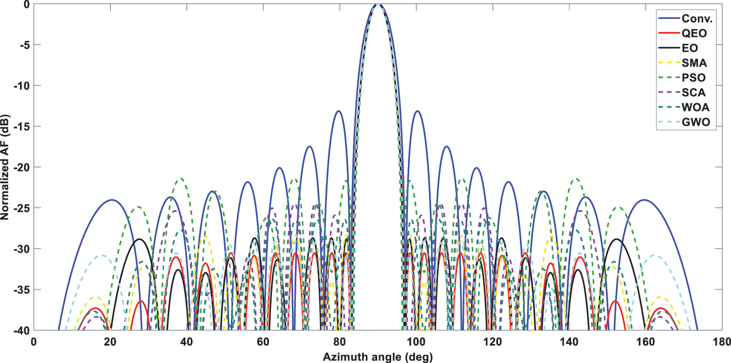
Figure 4: 2D beam patterns for 24-elements LAA

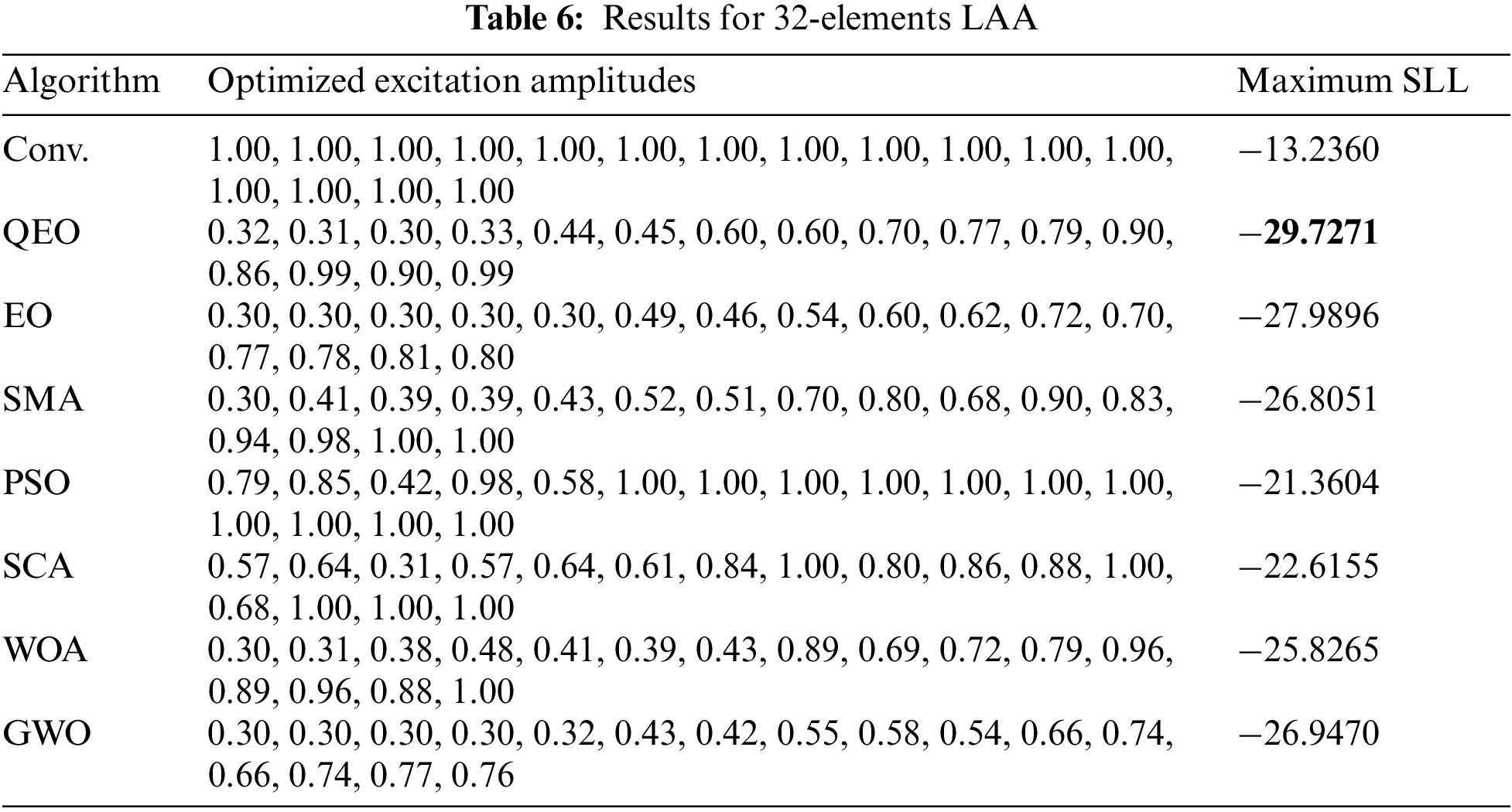
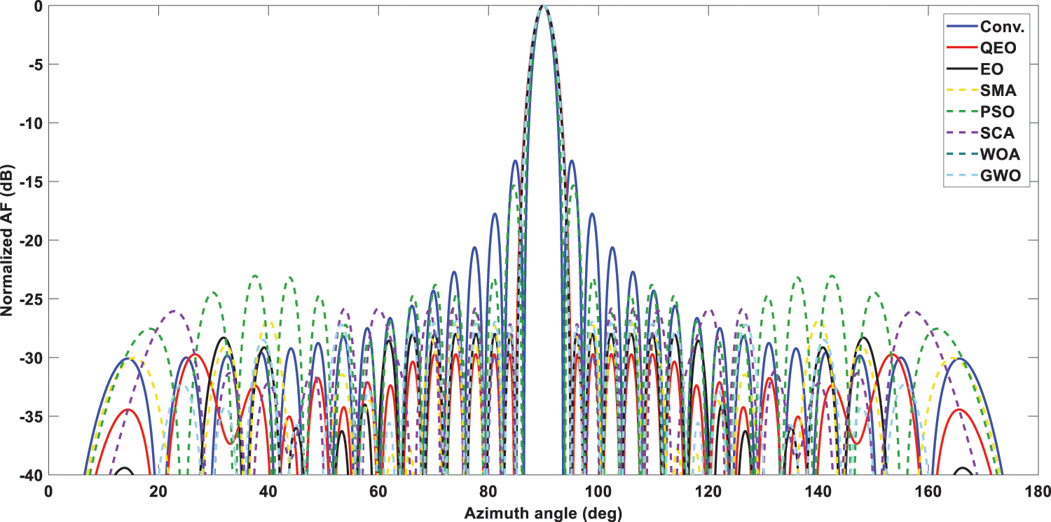
Figure 5: 2D beam patterns for 32-elements LAA

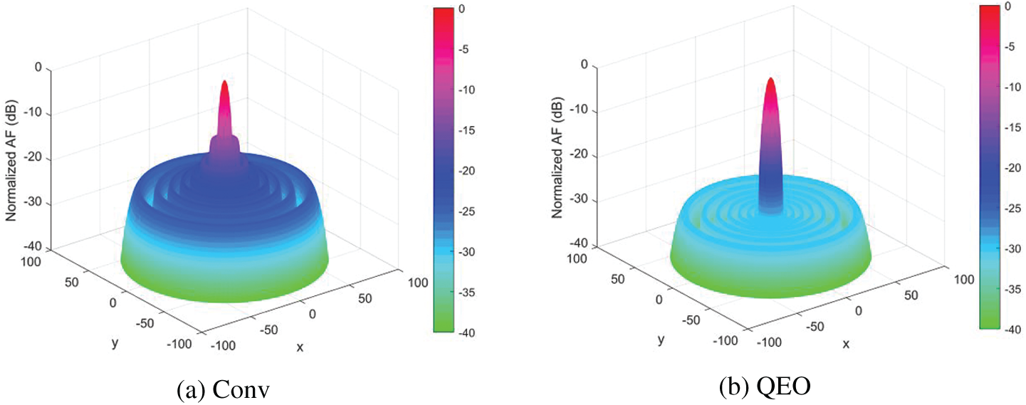
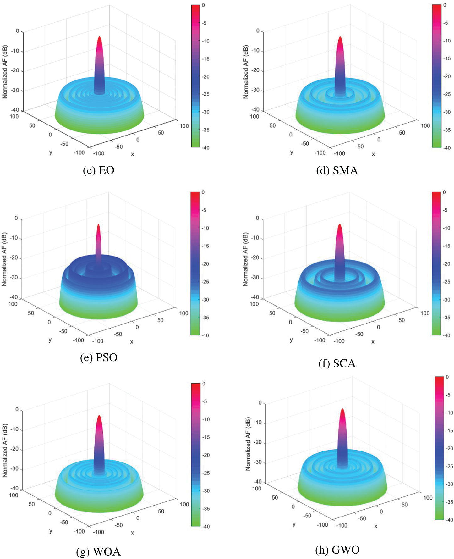
Figure 6: 3D beam patterns for 16-elements LAA

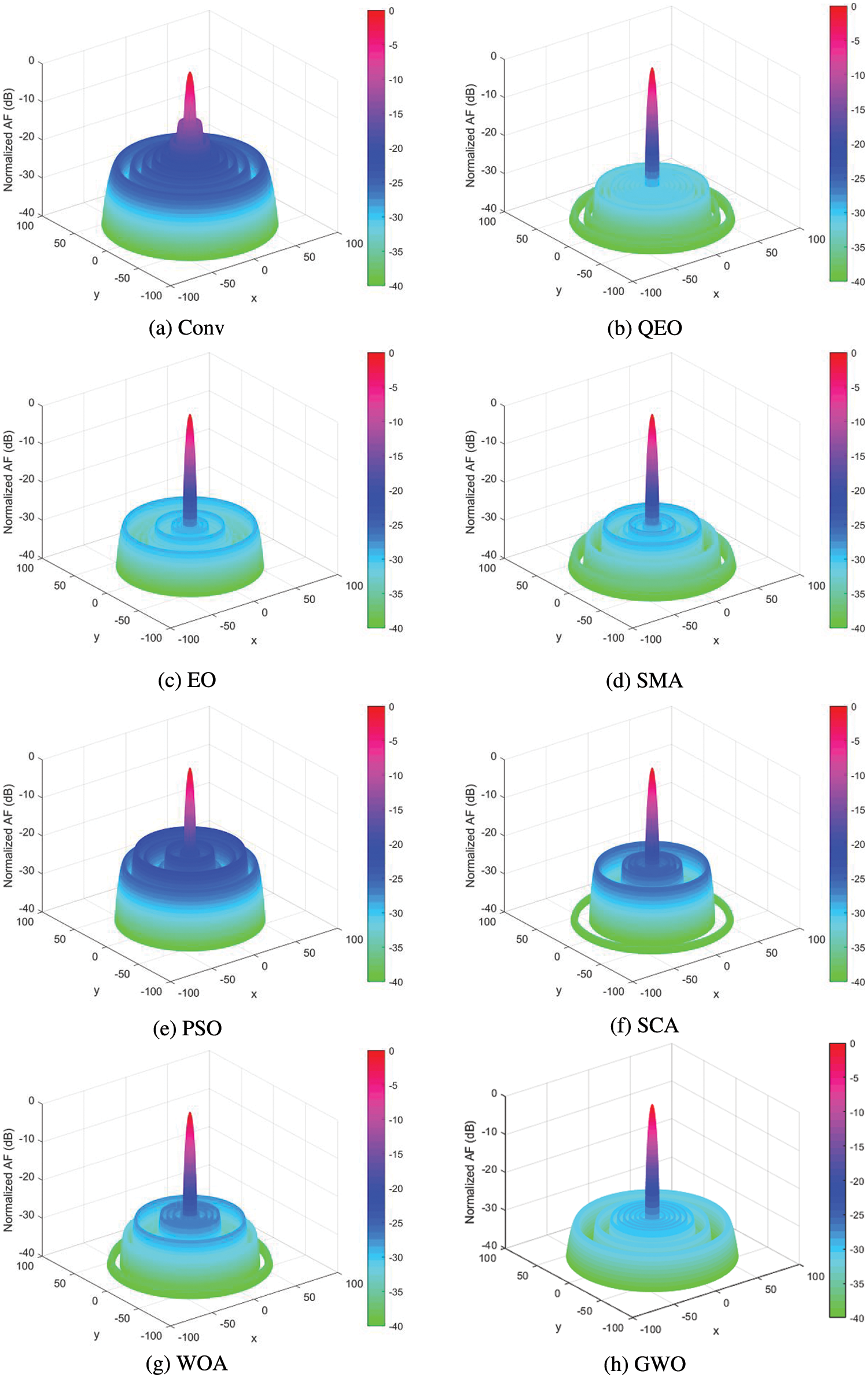
Figure 7: 3D beam patterns for 32-elements LAA

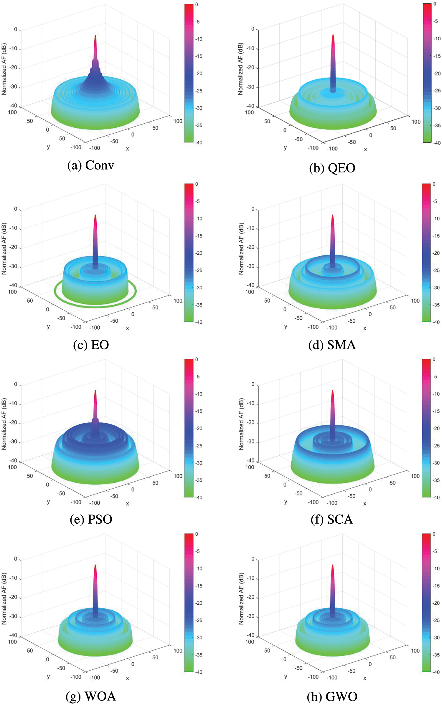
Figure 8: 3D beam patterns for 32-elements LAA

6.4 Convergence Analysis

In this section, we analyze the convergence curves of different algorithms for LAA optimization of SLL with the different number of array elements. The convergence curves give a good indication of the optimization ability of the quantum equilibrium optimizer as well as other methods. The algorithm's search ability is related to its exploration ability and exploration ability. A stronger exploration ability makes the algorithm converge easily and early, while a stronger exploration ability decreases the convergence speed of the algorithm. As seen in Figs. 9–11, the best convergence curves are obtained for QEO in all three different systems, and the convergence speed and the accuracy of the searchare the best. Compared with the basic equilibrium optimizer, the quantum coding-based strategy improves the population diversity avoiding the algorithm from falling into premature convergence and improves the optimization accuracy of the equilibrium optimizer. The particles in the quantum equilibrium pool undergo quantum mutation to produce phase angle increments and update the probability operators through a quantum rotation gate. Based on this method, QEO can effectively escape from local optima in the late iterative stage and avoid overcrowding of the quantum population.

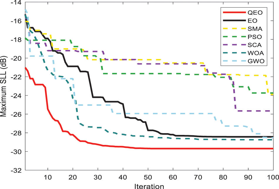
Figure 9: Convergence curve for 16-elements LAA

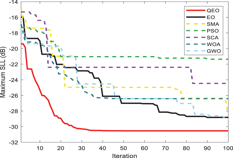
Figure 10: Convergence curve for 24-elements LAA

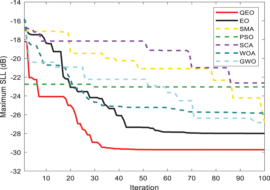
Figure 11: Convergence curve for 24-elements LAA

6.5 Stability Test and Statistical Analysis

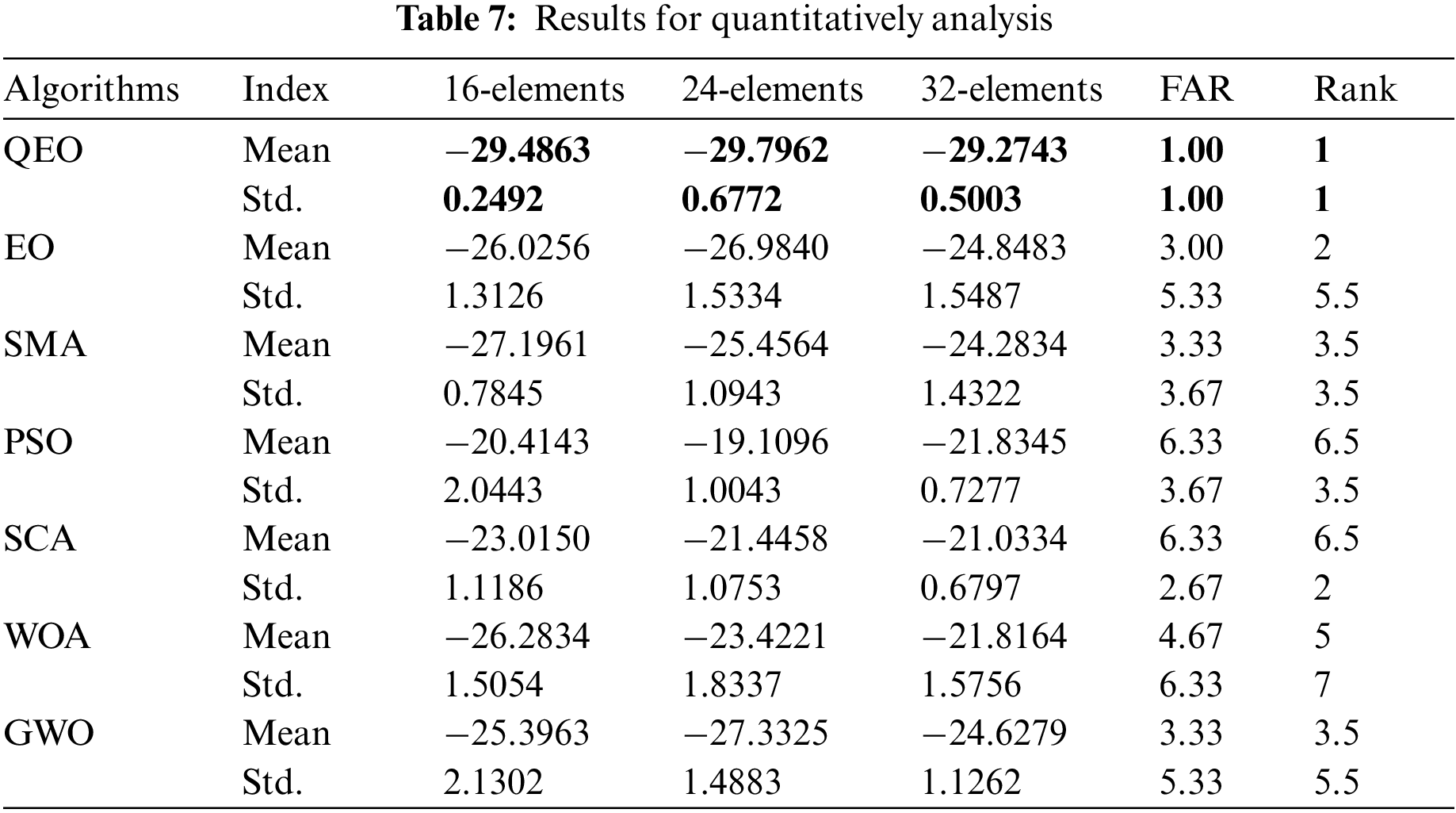
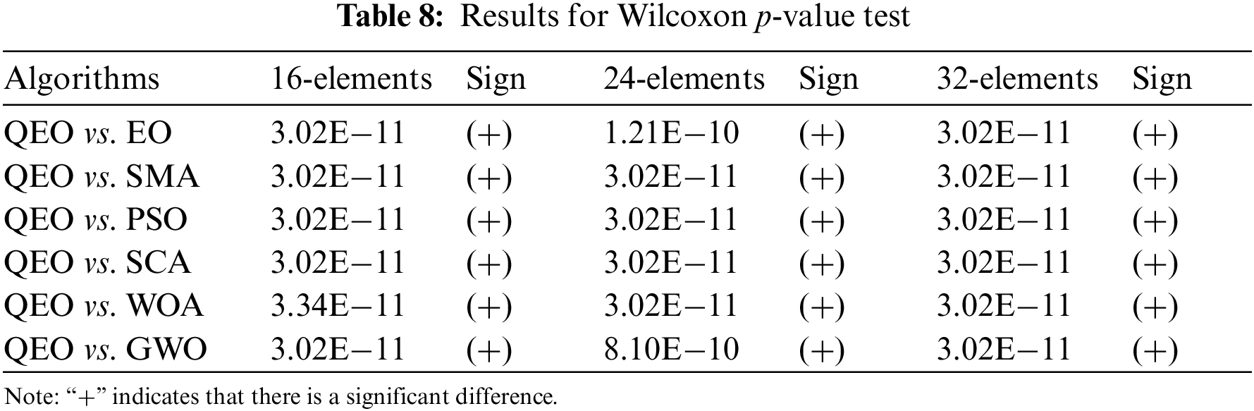
The intelligent optimization algorithm is stochastic, so that the computational results are different each time. In this section, we analyze the computational stability and the optimization performance of the algorithms. In order to observe the fluctuation of the data more intuitively, the optimization results of different optimization algorithms in three different LAA for thirty times are plotted, as shown in Figs. 12–14. It can be clearly observed from the figure that the mean value of QEO is the lowest located at the bottom of the picture, indicating that the proposed method has higher solution accuracy and robustness in optimizing the maximum SLL reduction problem. In order to quantitatively analyze the computational stability of the algorithm, the mean and standard deviation of different algorithms in the three test systems are shown in Table 7, and the method of Friedman’s average ranking is used for statistical analysis of the experiment result. FAR represents the score of Friedman’s average ranking, and Rank represents the ranking of statistical analysis of different algorithms. In order to verify whether the proposed method is significantly different from other optimization methods, the statistical analysis method of Wilcoxon p-value test is used in this section, and the results show that QEO significantly outperforms other methods in Table 8. The algorithm significantly outperforms the EO, SMA, PSO, SCA, WOA, and GWO algorithms in solving the linear antenna array optimization problem, which proves that the proposed quantum equilibrium optimizer has strong optimization capability.

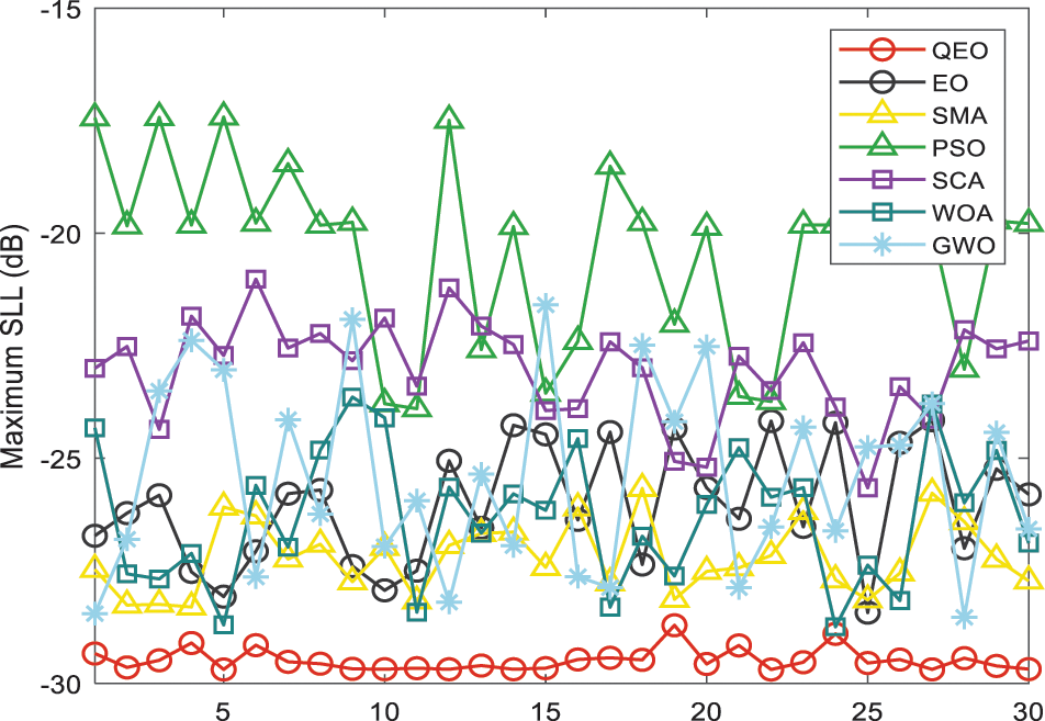
Figure 12: 30 results distribution on 16-elements LAA

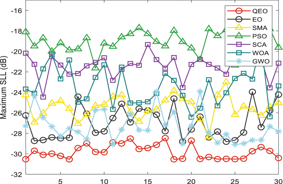
Figure 13: 30 results distribution on 24-elements LAA

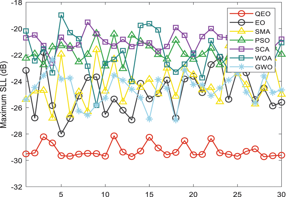
Figure 14: 30 results distribution on 32-elements LAA

7  Conclusions and Future Works

In this paper, a quantum-inspired equilibrium optimizer algorithm is proposed to introduce the idea of quantum computing combined with the equilibrium optimizer to solve the optimization problem of linear antenna arrays. For the defects of premature convergence and easily fall into the local optimum of the basic equilibrium optimizer, a quantum equilibrium pool strategy inspired by quantum computing is proposed and a quantum rotation gate strategy is introduced to improve the EO. On the other hand, the effectiveness and robustness of the proposed algorithm in this problem are verified by testing the solving maximum SLL capability in an antenna array with three different numbers of array elements. The quantum equilibrium optimizer is compared with the classical PSO, EO, SMA, WOA, GWO, and SCA, using the array element excitation as the design variable and the reduction of the maximum SLL of the antenna array as the objective. The experimental results showed that QEO has higher convergence speed and better search accuracy than other compared algorithms and is very competitive in this problem. And it is significantly better than the basic equilibrium optimizer, which verifies the effectiveness of the improvement. In future works, we will try to use the quantum equilibrium optimizer in other antenna array optimization problems. For example, for circular antenna array optimization, the algorithm is discredited to solve the sparse antenna array optimization problem, and multiple objectives are considered to be optimized simultaneously.

Funding Statement: This work was supported by the National Science Foundation of China under Grant No. 62066005, and Project of the Guangxi Science and Technology under Grant No. AD21196006.

Conflicts of Interest: The authors declare that they have no known competing financial interests or personal relationships that could have appeared to influence the work reported in this paper.

References

1. Chettri, L., Bera, R. (2020). A comprehensive survey on Internet of Things (IoT) toward 5G wireless systems. IEEE Internet of Things Journal, 7(1), 16–32. https://doi.org/10.1109/JIOT.2019.2948888 [Google Scholar] [CrossRef]

2. Pradhan, H., Mangaraj, B. B., Kumar, B. S. (2019). Antenna array optimization for smart antenna technology using whale optimization algorithm. 2019 IEEE Indian Conference on Antennas and Propagation, India. [Google Scholar]

3. Lin, M., Gao, Y., Liu, P., Liu, J. (2017). Theoretical analyses and design of circular array to generate orbital angular momentum. IEEE Transactions on Antennas and Propagation, 65(7), 3510–3519. https://doi.org/10.1109/TAP.2017.2700160 [Google Scholar] [CrossRef]

4. Kummer, W. H. (1992). Basic array theory. Proceedings of the IEEE, 80(1), 127–140. https://doi.org/10.1109/5.119572 [Google Scholar] [CrossRef]

5. Ram, G., Mandal, D., Ghoshal, S. P., Kar, R. (2017). Nature-inspired algorithm-based optimization for beamforming of linear antenna array system. Nature-Inspired Computing and Optimization, 10, 185–215. https://doi.org/10.1007/978-3-319-50920-4 [Google Scholar] [CrossRef]

6. Koziel, S., Stanislav, O. (2019). Simulation-based optimization of antenna arrays. Reykjavik University, Iceland: World Scientific. [Google Scholar]

7. Holland, J. H. (1973). Genetic algorithms and the optimal allocation of trials. SIAM Journal on Computing, 2(2), 88–105. https://doi.org/10.1137/0202009 [Google Scholar] [CrossRef]

8. Vent, W. (1975). Rechenberg, Ingo, Evolutionsstrategie—Optimierung technischer Systeme nach Prinzipien der biologischen Evolution. 170 S. mit 36 Abb. Frommann-Holzboog-Verlag. Stuttgart 1973. Broschiert. Feddes Repertorium, 86(5), 337. [Google Scholar]

9. Storn, R. (1997). Differential evolution–A simple and efficient heuristic for global optimization over continuous spaces. Journal of Global Optimization, 11(4), 341–359. https://doi.org/10.1023/A:1008202821328 [Google Scholar] [CrossRef]

10. Yao, X. (1999). Evolutionary programming made faster. IEEE Transactions on Evolutionary Computation, 3(2), 82−102. [Google Scholar]

11. Kennedy, J., Eberhart, R. (1995). Particle swarm optimization. International Conference on Neural Networks, 4, 1942–1948. https://doi.org/10.1109/ICNN.1995.488968 [Google Scholar] [CrossRef]

12. Akay, B., Karaboga, D., Gorkemli, B., Kaya, E. (2021). A survey on the Artificial Bee Colony algorithm variants for binary, integer and mixed integer programming problems. Applied Soft Computing, 106(3), 10735. https://doi.org/10.1016/j.asoc.2021.107351 [Google Scholar] [CrossRef]

13. Braik, M. S. (2021). Chameleon swarm algorithm: A bio-inspired optimizer for solving engineering design problems. Expert Systems with Applications, 174(1), 114685. https://doi.org/10.1016/j.eswa.2021.114685 [Google Scholar] [CrossRef]

14. Sulaiman, M. H., Mustaffa, Z., Saari, M. M., Daniyal, H. (2020). Barnacles mating optimizer: A new bio-inspired algorithm for solving engineering optimization problems. Engineering Applications of Artificial Intelligence, 87, 103330. https://doi.org/10.1016/j.engappai.2019.103330 [Google Scholar] [CrossRef]

15. Mirjalili, S., Lewis, A. (2016). The whale optimization algorithm. Advances in Engineering Software, 95(12), 51–67. https://doi.org/10.1016/j.advengsoft.2016.01.008 [Google Scholar] [CrossRef]

16. Mirjalili, S., Gandomi, A. H., Mirjalili, S. Z., Saremi, S., Faris, H. et al. (2017). Salp swarm algorithm: A bio-inspired optimizer for engineering design problems. Advances in Engineering Software, 114, 163–191. https://doi.org/10.1016/j.advengsoft.2017.07.002 [Google Scholar] [CrossRef]

17. Mirjalili, S., Mirjalili, S. M., Lewis, A. (2014). Grey wolf optimizer. Advances in Engineering Software, 69, 41–61. https://doi.org/10.1016/j.advengsoft.2013.12.007 [Google Scholar] [CrossRef]

18. Li, S., Chen, H., Wang, M., Heidari, A. A., Mirjalili, S. (2020). Slime mould algorithm: A new method for stochastic optimization. Future Generation Computer Systems, 111(Supplement C), 300–323. https://doi.org/10.1016/j.future.2020.03.055 [Google Scholar] [CrossRef]

19. Anita, Y. A. (2019). AEFA: Artificial electric field algorithm for global optimization. Swarm and Evolutionary Computation, 48(1), 93–108. https://doi.org/10.1016/j.swevo.2019.03.013 [Google Scholar] [CrossRef]

20. Faramarzi, A., Heidarinejad, M., Stephens, B., Mirjalili, S. (2020). Equilibrium optimizer: A novel optimization algorithm. Knowledge-Based Systems, 191, 105190. https://doi.org/10.1016/j.knosys.2019.105190 [Google Scholar] [CrossRef]

21. Kirkpatrick, S. (1984). Optimization by simulated annealing: Quantitative studies. Journal of Statistical Physics, 34(5–6), 975–986. https://doi.org/10.1007/BF01009452 [Google Scholar] [CrossRef]

22. Erol, O. K., Eksin, I. (2006). A new optimization method: Big Bang–Big Crunch. Advances in Engineering Software, 37(2), 106–111. https://doi.org/10.1016/j.advengsoft.2005.04.005 [Google Scholar] [CrossRef]

23. Shareef, H., Ibrahim, A. A., Mutlag, A. H. (2015). Lightning search algorithm. Applied Soft Computing, 36(2011), 315–333. https://doi.org/10.1016/j.asoc.2015.07.028 [Google Scholar] [CrossRef]

24. Patel, V. K., Savsani, V. J. (2015). Heat transfer search (HTSA novel optimization algorithm. Informing Science, 324(2), 217–246. https://doi.org/10.1016/j.ins.2015.06.044 [Google Scholar] [CrossRef]

25. Rao, R. V., Savsani, V. J., Vakharia, D. P. (2011). Teaching-learning-based optimization: A novel method for constrained mechanical design optimization problems. Computer-Aided Design, 43(3), 303–315. https://doi.org/10.1016/j.cad.2010.12.015 [Google Scholar] [CrossRef]

26. Shi, Y. (2011). Brain storm optimization algorithm. International Conference on Swarm Intelligence, Heidelberg, Berlin. [Google Scholar]

27. Moghdani, R., Salimifard, K. (2018). Volleyball premier league algorithm. Applied Soft Computing, 64(5), 161–185. https://doi.org/10.1016/j.asoc.2017.11.043 [Google Scholar] [CrossRef]

28. Wolpert, D. H., Macready, W. G. (1997). No free lunch theorems for optimization. IEEE Transactions on Evolutionary Computation, 1(1), 67–82. https://doi.org/10.1109/4235.585893 [Google Scholar] [CrossRef]

29. Abdel-Basset, M., Mohamed, R., Mirjalili, S., Chakrabortty, R. K., Ryan, M. J. (2020). Solar photovoltaic parameter estimation using an improved equilibrium optimizer. Solar Energy, 209(3), 694–708. https://doi.org/10.1016/j.solener.2020.09.032 [Google Scholar] [CrossRef]

30. Gupta, S., Deep, K., Mirjalili, S. (2020). An efficient equilibrium optimizer with mutation strategy for numerical optimization. Applied Soft Computing, 96(1), 106542. https://doi.org/10.1016/j.asoc.2020.106542 [Google Scholar] [CrossRef]

31. Gao, Y., Zhou, Y., Luo, Q. (2020). An efficient binary equilibrium optimizer algorithm for feature selection. IEEE Access, 8, 140936–140963. https://doi.org/10.1109/ACCESS.2020.3013617 [Google Scholar] [CrossRef]

32. Wunnava, A., Naik, M. K., Panda, R., Jena, B., Abraham, A. (2020). A novel interdependence based multilevel thresholding technique using adaptive equilibrium optimizer. Engineering Applications of Artificial Intelligence, 94, 103836. https://doi.org/10.1016/j.engappai.2020.103836 [Google Scholar] [CrossRef]

33. Abdul-hamied, D. T., Shaheen, A. M., Salem, W. A., Gabr, W. I., El-sehiemy, R. A. (2020). Equilibrium optimizer based multi dimensions operation of hybrid AC/DC grids. Alexandria Engineering Journal, 59(6), 4787–4803. https://doi.org/10.1016/j.aej.2020.08.043 [Google Scholar] [CrossRef]

34. Fan, Q., Huang, H., Yang, K., Zhang, S., Yao, L. et al. (2021). A modified equilibrium optimizer using opposition-based learning and novel update rules. Expert Systems with Applications, 170(9), 114575. https://doi.org/10.1016/j.eswa.2021.114575 [Google Scholar] [CrossRef]

35. Elsheikh, A. H., Shehabeldeen, T. A., Zhou, J., Showaib, E., AbdElaziz, M. (2021). Prediction of laser cutting parameters for polymethylmethacrylate sheets using random vector functional link network integrated with equilibrium optimizer. Journal of Intelligent Manufacturing, 32(5), 1377–1388. https://doi.org/10.1007/s10845-020-01617-7 [Google Scholar] [CrossRef]

36. Yin, S., Luo, Q., Zhou, Y. (2022). EOSMA: An equilibrium optimizer slime mould algorithm for engineering design problems. Arabian Journal for Science and Engineering, 47(8), 10115–10146. https://doi.org/10.1007/s13369-021-06513-7 [Google Scholar] [CrossRef]

37. Tang, A. D., Han, T., Zhou, H., Xie, L. (2021). An improved equilibrium optimizer with application in unmanned aerial vehicle path planning. Sensors, 21(5), 1814. https://doi.org/10.3390/s21051814 [Google Scholar] [PubMed] [CrossRef]

38. Abdel-Basset, M., Mohamed, R., Mirjalili, S., Chakrabortty, R. K., Ryan, M. J. (2021). MOEO-EED: A multi-objective equilibrium optimizer with exploration-exploitation dominance strategy. Knowledge-Based Systems, 214(6), 106717. https://doi.org/10.1016/j.knosys.2020.106717 [Google Scholar] [CrossRef]

39. Panduro, M. A., Mendez, A. L., Dominguez, R., Romero, G. (2006). Design of non-uniform circular antenna arrays for side lobe reduction using the method of genetic algorithms. AEU–International Journal of Electronics Communication, 60(10), 713–717. https://doi.org/10.1016/j.aeue.2006.03.006 [Google Scholar] [CrossRef]

40. Khodier, M. M., Christodoulou, C. G. (2005). Linear array geometry synthesis with minimum sidelobe level and null control using particle swarm optimization. IEEE Transactions on Antennas and Propagation, 53(8), 2674–2679. https://doi.org/10.1109/TAP.2005.851762 [Google Scholar] [CrossRef]

41. Guney, K., Onay, M. (2010). Bees algorithm for interference suppression of linear antenna arrays by controlling the phase-only and both the amplitude and phase. Expert Systems with Applications, 37(4), 3129–3135. https://doi.org/10.1016/j.eswa.2009.09.072 [Google Scholar] [CrossRef]

42. Singh, U., Kumar, H., Kamal, T. S. (2010). Linear array synthesis using biogeography based optimization. Progress in Electromagnetics Reserch M, 11, 25–36. https://doi.org/10.2528/PIERM09120201 [Google Scholar] [CrossRef]

43. Pappula, L., Ghosh, D. (2014). Linear antenna array synthesis using cat swarm optimization. AEU–International Journal of Electronics Communication, 68(6), 540–549. https://doi.org/10.1016/j.aeue.2013.12.012 [Google Scholar] [CrossRef]

44. Singh, U., Rattan, M. (2014). Design of linear and circular antenna arrays using cuckoo optimization algorithm. Progress in Electromagnetics Reserch C, 46, 1–11. https://doi.org/10.2528/PIERC13110902 [Google Scholar] [CrossRef]

45. Dib, N. I. (2016). Design of linear antenna arrays with low side lobes level using symbiotic organisms search. Progress in Electromagnetics Reserch B, 68, 55–71. [Google Scholar]

46. Saxena, P., Kothari, A. (2016). Optimal pattern synthesis of linear antenna array using grey wolf optimization algorithm. International Journal of Antennas and Propagation, 2016(15), 1–11. https://doi.org/10.1155/2016/1205970 [Google Scholar] [CrossRef]

47. Salgotra, R., Singh, U., Sharma, S. (2020). On the improvement in grey wolf optimization. Neural Computing & Applications, 32(8), 3709–3748. https://doi.org/10.1007/s00521-019-04456-7 [Google Scholar] [CrossRef]

48. Wu, H., Yan, Y., Liu, C., Zhang, J. (2017). Pattern synthesis of sparse linear arrays using spider monkey optimization. IEICE Transactions on Communications, E100.B(3), 426–432. https://doi.org/10.1587/transcom.2016EBP3203 [Google Scholar] [CrossRef]

49. Sun, G., Liu, Y., Li, H., Liang, S., Wang, A. et al. (2018). An antenna array sidelobe level reduction approach through invasive weed optimization. International Journal of Antennas and Propagation, 2018(4), 1–16. https://doi.org/10.1155/2018/4867851 [Google Scholar] [CrossRef]

50. Durmus, A., Kurban, R. (2021). Optimum design of linear and circular antenna arrays using equilibrium optimization algorithm. International Journal of Microwave and Wireless Technologies, 13(9), 986–997. https://doi.org/10.1017/S1759078720001774 [Google Scholar] [CrossRef]

51. Sharaqa, A., Dib, N. (2014). Design of linear and elliptical antenna arrays using biogeography based optimization. Arabian Journal for Science and Engineering, 39(4), 2929–2939. https://doi.org/10.1007/s13369-013-0794-8 [Google Scholar] [CrossRef]

52. Das, A., Mandal, D., Ghoshal, S. P., Kar, R. (2019). Moth flame optimization based design of linear and circular antenna array for side lobe reduction. International Journal of Numerical Modeling-Electronic Networks Devices and Fields, 32(1), e2486. https://doi.org/10.1002/jnm.2486 [Google Scholar] [CrossRef]

53. Subhashini, K. R. (2020). Runner-root algorithm to control sidelobe level and null depths in linear antenna arrays. Arabian Journal for Science and Engineering, 45(3), 513–1529. https://doi.org/10.1007/s13369-019-04051-x [Google Scholar] [CrossRef]

54. Almagboul, M. A., Shu, F., Qian, Y., Zhou, X., Wang, J. et al. (2019). Atom search optimization algorithm based hybrid antenna array receive beamforming to control sidelobe level and steering the null. AEU–International Journal of Electronics Communication, 111(9), 152854. https://doi.org/10.1016/j.aeue.2019.152854 [Google Scholar] [CrossRef]

55. Singh, H., Abouhawwash, M., Mittal, N., Salgotra, R., Mahajan, S. et al. (2022). Performance evaluation of non-uniform circular antenna array using integrated harmony search with differential evolution based naked mole rat algorithm. Expert Systems with Applications, 189(6), 116146. https://doi.org/10.1016/j.eswa.2021.116146 [Google Scholar] [CrossRef]

56. Vegesna, N., Yamuna, G., Terlapu, S. K. (2022). Design of linear array for shaped beams using enhanced flower pollination optimization algorithm. Soft Computing, 26(12), 5805–5813. https://doi.org/10.1007/s00500-022-07146-0 [Google Scholar] [CrossRef]

57. Liang, S., Fang, Z., Sun, G., Qu, G. (2022). Biogeography-based optimization with adaptive migration and adaptive mutation with its application in sidelobe reduction of antenna arrays. Applied Soft Computing, 121(2), 108772. https://doi.org/10.1016/j.asoc.2022.108772 [Google Scholar] [CrossRef]

58. Deutsch, D. (1985). Quantum theory, the church-turing principle and the universal quantum computer. Proceedings of the Royal Society of London, 400(1818), 97–117. [Google Scholar]

59. Yu, C., Cai, Z., Ye, X., Wang, M., Zhao, X. et al. (2020). Quantum-like mutation-induced dragonfly-inspired optimization approach. Mathematics and Computers in Simulation, 178(9), 259–289. https://doi.org/10.1016/j.matcom.2020.06.012 [Google Scholar] [CrossRef]

60. Zhang, S., Zhou, G., Zhou, Y., Luo, Q. (2021). Quantum-inspired satin bowerbird algorithm with bloch spherical search for constrained structural optimization. Journal of Industrial and Management Optimization, 17(6), 3509–3523. https://doi.org/10.3934/jimo.2020130 [Google Scholar] [CrossRef]

61. Deng, W., Shang, S., Cai, X., Zhao, H., Zhou, Y. et al. (2021). Quantum differential evolution with cooperative co-evolution framework and hybrid mutation strategy for large scale optimization. Knowledge-Based Systems, 224(1), 107080. https://doi.org/10.1016/j.knosys.2021.107080 [Google Scholar] [CrossRef]

62. Zhou, Y., Bao, Z., Wang, R., Qiao, S. (2015). Quantum wind driven optimization for unmanned combat air vehicle path planning. Applied Sciences, 5(4), 1457–1483. https://doi.org/10.3390/app5041457 [Google Scholar] [CrossRef]

63. Dos, L., Coelho, S. (2010). Gaussian quantum-behaved particle swarm optimization approaches for constrained engineering design problems. Expert Systems with Applications, 37(2), 1676–1683. https://doi.org/10.1016/j.eswa.2009.06.044 [Google Scholar] [CrossRef]

64. Zou, F., Wang, L., Hei, X., Chen, D., Yang, D. (2014). Teaching-learning-based optimization with dynamic group strategy for global optimization. Informing Science, 273(1), 112–131. https://doi.org/10.1016/j.ins.2014.03.038 [Google Scholar] [CrossRef]

65. Yu, C., Heidari, A. A., Xue, X., Zhang, L., Chen, H. et al. (2021). Boosting quantum rotation gate embedded slime mould algorithm. Expert Systems with Applications, 181(8), 115082. https://doi.org/10.1016/j.eswa.2021.115082 [Google Scholar] [CrossRef]

66. Cui, X., Luo, Q., Zhou, Y., Deng, W., Yin, S. (2022). Quantum-inspired moth-flame optimizer with enhanced local search strategy for cluster analysis. Frontiers in Bioengineering and Biotechnology, 10, 908356. https://doi.org/10.3389/fbioe.2022.908356 [Google Scholar] [PubMed] [CrossRef]

67. Li, N., Zhou, G., Zhou, Y., Deng, W., Luo, Q. (2022). Extracting unknown parameters of proton exchange membrane fuel cells using quantum encoded pathfinder algorithm. Frontiers in Energy Research, 10, 964042. https://doi.org/10.3389/fenrg.2022.964042 [Google Scholar] [CrossRef]

68. Ho, S. L., Yang, S., Ni, G., Huang, J. (2013). A quantum-based particle swarm optimization algorithm applied to inverse problems. IEEE Transaction on Magnetics, 49(5), 2069–2072. https://doi.org/10.1109/TMAG.2013.2237760 [Google Scholar] [CrossRef]

69. Patidar, H., Mahanti, G. K. (2017). Quantum particle swarm optimization for synthesis of non-uniformly spaced linear arrays with broadband frequency invariant pattern. Journal of Microwaves, Optoelectronics and Electromagnetic Applications, 16(3), 602–614. https://doi.org/10.1590/2179-10742017v16i3790 [Google Scholar] [CrossRef]

70. Gao, H. Y., Zhang, X. T., Du, Y. N., Diao, M. (2017). Quantum-inspired teaching-learning-based optimization for linear array pattern synthesis. In: Liang, Q., Mu, J., Jia, M., Wang, W., Feng,X. et al. (Eds.Communications, signal processing, and systems, pp. 2106–2115. Singapore: Springer. https://doi.org/10.1007/978-981-10-6571-2_257 [Google Scholar] [CrossRef]

71. Liu, M., Yuan, C., Li, S., Wu, H. (2006). Radiation pattern synthesis for adaptive antenna arrays using improved quantum genetic algorithm. 2006 7th International Symposium on Antennas, Propagation & EM Theory, Guilin, China. [Google Scholar]

72. Mikki, S., Kishk, A. (2006). Quantum particle swarm optimization for electromagnetics. IEEE Transactions on Antenna and Propagation, 54(10), 2764–2775. https://doi.org/10.1109/TAP.2006.882165 [Google Scholar] [CrossRef]

73. Weng, W. C., Yang, F., Elsherbeni, A. Z. (2007). Linear antenna array synthesis using taguchi’s method: A novel optimization technique in electromagnetics. IEEE Transactions on Antennas and Propagation, 55(3), 723–730. https://doi.org/10.1109/TAP.2007.891548 [Google Scholar] [CrossRef]

74. Mirjalili, S. (2016). SCA: A sine cosine algorithm for solving optimization problems. Knowledge-Based Systems, 96(63), 120–133. https://doi.org/10.1016/j.knosys.2015.12.022 [Google Scholar] [CrossRef]