Comparison Study and Forensic Analysis between Experiment and Coupled Dynamics Simulation for Submerged Floating Tunnel Segment with Free Ends under Wave Excitations

1  Introduction

A submerged floating tunnel (SFT) is a novel underwater structure proposed to cross deep-water waterways. It is a simple structure comprised of a long tunnel made of concrete, steel, or concrete-steel hybrid and station-keeping systems such as mooring lines and tendons. Since the structure is floating and deeply submerged, it is known to be relatively much safer against waves and earthquakes. It does not obstruct surface maritime traffic, and modular construction can be applied to the entire length [1]. In this regard, there have been active investigations of this structure, which encompasses Høgsfjord/Bjørnafjord in Norway [2], the Strait of Messina in Italy [3], Funka Bay in Japan [4], Qiandao Lake in China [5], and the Mokpo-Jeju SFT in South Korea [6,7]. The accumulated knowledge through those studies is expected to contribute to the first real-scale construction in the near future.

An experimental study is one of the fundamental approaches to checking the global performance of the structures that are supposed to be deployed in the ocean. However, the current state of the art shows that there exist insufficient experimental data available for SFT due to its relatively short period of relevant research, which results in difficulties in the validation of numerical simulations. Regarding experimental studies of SFT under wave excitations, Kunisu et al. [8] investigated the effect of different mooring types on dynamic behaviors and mooring tension. Kunisu [9] evaluated wave forces on SFTs of different shapes and sizes. Oh et al. [10] checked the influences of different mooring types, water depths, and buoyancy-to-weight ratios (BWRs) on global performance. Seo et al. [11] compared their simplified numerical simulation model with experiments. Li et al. [12] studied pressure characteristics of different tunnel shapes with pressure sensors around SFT. Yang et al. [13] conducted parametric studies with varying BWRs, water depths, wave heights, inclination angles of mooring lines, and wave periods. All of the above examples only considered regular waves in their experiment/analysis, which means that SFT’s motion characteristics measured under random waves are still rare. The previous studies described above were conducted in 2D wave tanks, and the tunnel segment was made of acrylic or steel tube moored by steel rope. In addition to dynamics under wave excitations, there were other experimental studies. Deng et al. [14] and Deng et al. [15] studied drag forces and vortex-induced vibrations under steady current for dual-tube SFT. Xiang et al. [16] investigated transient responses under anchor-cable failure scenarios. Xiang et al. [17] conducted experiments with regard to SFT under moving loads. The structural characteristics of precast segment module joints were tested and evaluated [18].

Several comparative studies were also carried out to take advantage of those experimental data for the validation of developed numerical simulation tools. Cifuentes et al. [19] and Lee et al. [20] conducted a comparative study between the experiments by Oh et al. [10] and their numerical simulations under regular waves. Jin et al. [21] conducted free decay tests for a scaled model to obtain the natural frequencies and viscous damping coefficients to be used as inputs for their numerical simulations. Chen et al. [22] compared experimental results with CFD (computational fluid dynamics) simulations. Until recently, most of the experiments were for short rigid body segments, and the elastic behaviors of deformable long SFTs are not available yet, which is required to validate hydro-elastic numerical simulation programs.

In this study, a 3D-tank experiment is conducted, and the experimental results are compared with time-domain numerical simulations [23,24] under regular and irregular wave conditions. The experiments for a moored SFT are conducted in a 3D wave tank in KRISO (Korea Research Institute of Ships & Ocean Engineering). The experimental setup is modeled by the author-developed hydroelastic-simulation tool, and the experimental and simulation results are systematically compared. In the time-domain numerical simulations, the Cummins equation with 3D diffraction/radiation theory and independent Morison-equation-based formulas are employed to estimate hydrodynamic coefficients and wave excitation forces. Most previous experiments are conducted in 2D wave tanks using a short SFT section made of plastic tubes and wires as mooring system. However, in the present experiment, the tunnel is larger, longer, and made of concrete. Also, hollow-aluminum moorings are used as a mooring system to represent the characteristics of both mooring lines and tendons. The 3D wave tank is utilized to represent open water conditions better, and both regular and irregular wave conditions are considered. The free-free boundary condition is assumed at both ends of the tunnel section, which is the same setup both in experiment and simulation. In this case, rigid behaviors of the tunnel will mostly be seen, while elastic behaviors are hard to be observed.

2  Experimental Setup

In this section, the experimental setup for SFT is explained. The overall configuration and pictures for the experimental setup are presented in Fig. 1. 1:33.3-scale experiment is conducted in a KRISO’s 3D Ocean Engineering Basin with 56 m in length, 30 m in width, and 4.5 m in height. First, the tunnel body is made of concrete with a diameter of 0.6 m (20 m in real scale) as a hollow cylinder type (Fig. 2) with around 0.04-m wall thickness and 14317.71-kg mass. Both ends of the tunnel are sealed by transparent acrylic plates for waterproof purposes. Next, to fix the SFT on the bottom of the water tank, a fixed bottom structure is specially manufactured.

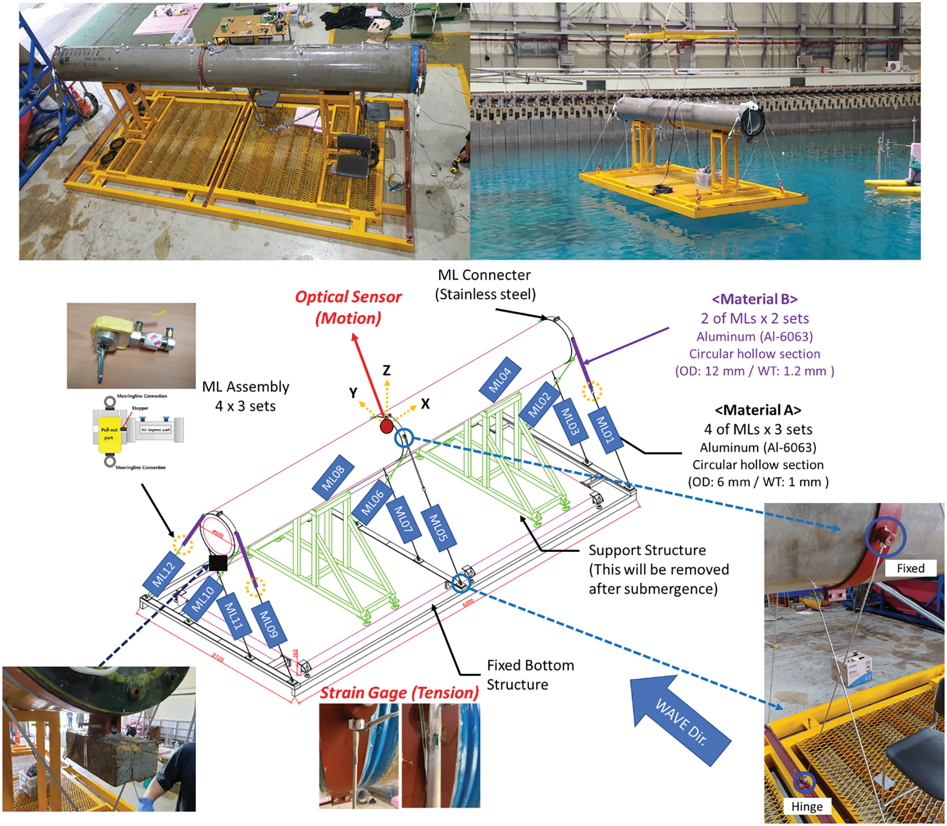
Figure 1: Picture and configuration of overall SFT system experiment model

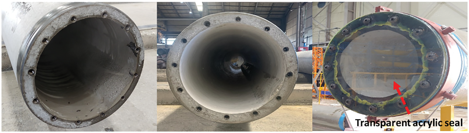
Figure 2: Picture of SFT system experiment model (tunnel body)

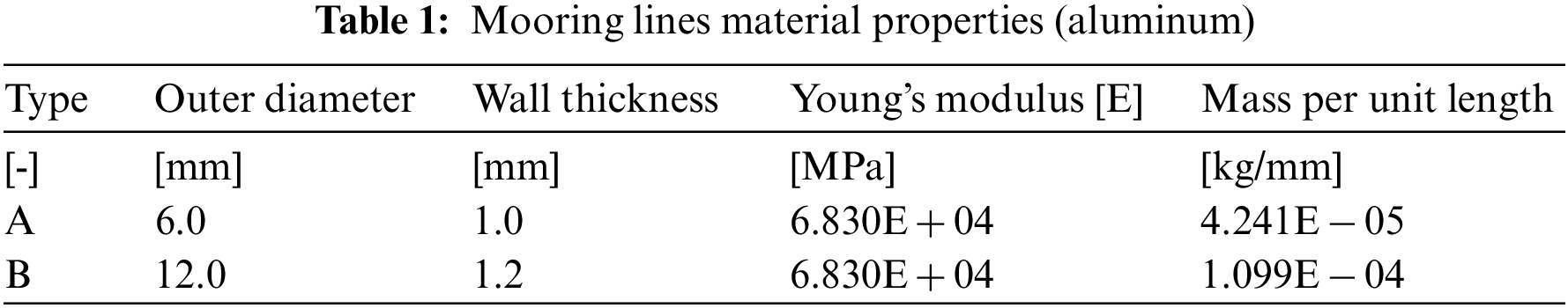
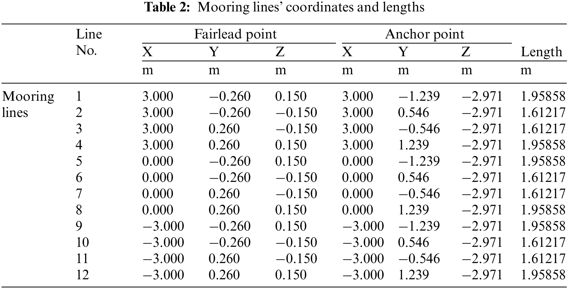
12 mooring lines (MLs) with a 60°-inclination angle are connected between the tunnel and fixed bottom structure—three mooring groups are located at the left end, middle, and right end of the tunnel, and each group consists of four MLs. To link the tunnel and mooring line, three circular type connectors made of stainless steel are attached along the main tunnel. In each group, inner mooring lines intersect each other, whereas outer lines are positioned toward the outside. As a mooring material property, aluminum is selected to simulate close to real-condition (1:33.3 scale). In detail, the mooring lines were scaled down according to the axial stiffness since the axial force (tension) is considered the governing factor in the behavior of mooring lines. Real-scale mooring lines are made of steel tube, but manufacturing a model-scale steel pipe with a small diameter and thickness is hard, which results in a relatively larger diameter/thickness aluminum pipe in our case. As shown in Table 1, each mooring line is made by a very thin aluminum (AL6063) pipe type (A type) while the top portion of four selected mooring lines (ML01, ML04, ML09, ML12) are replaced with other material properties (B type). Mooring lines’ coordinates and lengths are tabulated in Table 2. In the experimental setup, fixed BC (boundary condition) is used on the fairlead, whereas frictionless hinged BC is used on the bottom. Complex mooring assembly and materials, reflecting both tendon and mooring properties, are used to serve various testing purposes.

All the components are assembled in the air at first. The support structures at both ends ensure that the tunnel and MLs maintain their original positions in the air. After SFT is fully submerged, the support structures are removed. There is a slight misalignment of the tunnel in the water, which is compensated by a small additional weight attached to the left bottom of the tunnel. Submergence depth, a vertical distance between the water surface and the tunnel center, is 1.425 m (47.5 m in real scale) while water depth is 3.2 m (106 m in real scale). First, a series of impact loading tests are conducted. Afterward, two regular- and one irregular-wave tests are conducted, as shown in Table 3. The direction of waves is perpendicular to the longitudinal axis of the tunnel as the most severe condition.

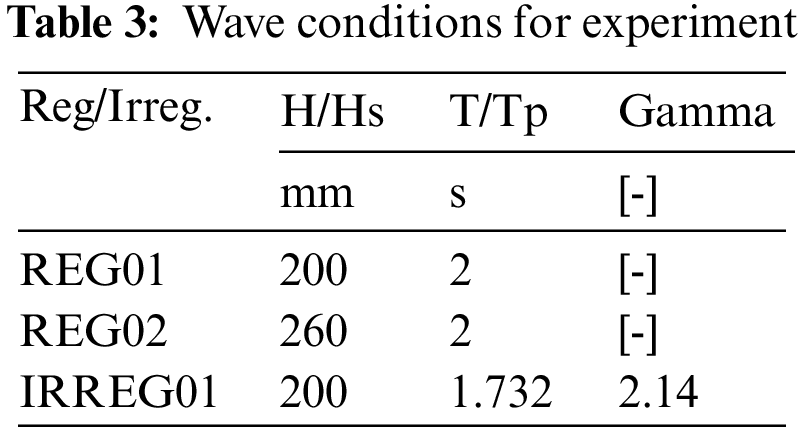
Fig. 3 shows the configuration of the wave tank, overall set-up, and wave elevation measurement locations. A total of five-wave probes are installed around the SFT system to measure wave elevation. An optical motion sensor is located at the upper middle part of the main tunnel to measure the dynamic response of the tunnel. Strain gages are attached to the top of each ML to measure mooring tension.

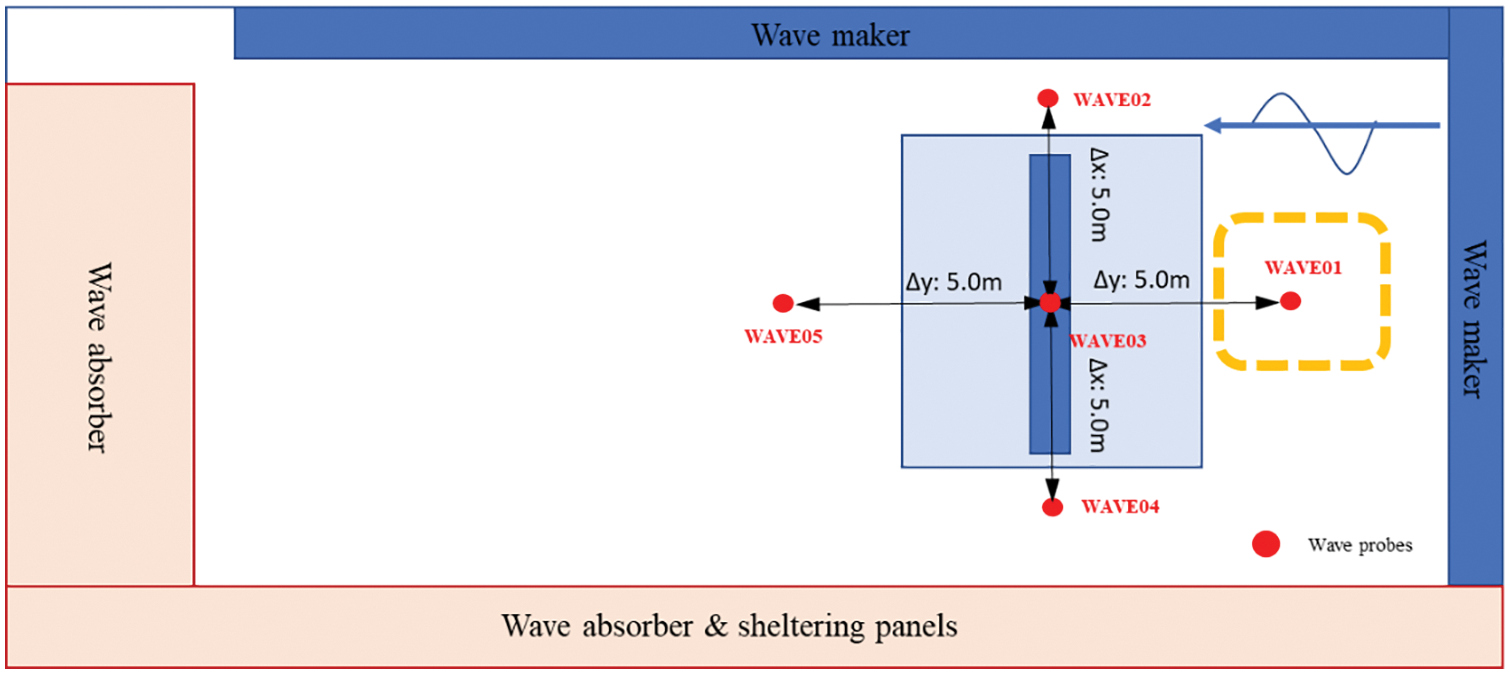
Figure 3: Configuration for wave tank and wave elevation measurement location

In fact, both ends of the actual SFT segment can be constrained by the adjacent tube or fixed station. However, in this experiment and numerical setup, this constrained effect was not considered (i.e., both ends’ BC is free) since we cannot introduce a very long tunnel section encompassing elastic behaviors with end restrictions due to the limited tank width.

3  Coupled Time-Domain Simulation

Tunnel-mooring coupled time-domain simulation is conducted by OrcaFlex, a well-known commercial program [25]. The typical time-domain equation of motion for the coupled system can be written as:

Mx¨+Kx=Fh+Fr+Fi(1)

where M and K are the system’s mass and structural stiffness matrices, respectively, x is the displacement vector, Fh is the hydrostatic force vector, Fr is the hydrodynamic force vector, and Fi is the constraint force vector due to coupling between the tunnel and mooring lines at their connection locations. The upper dots in the equations stand for the time derivative of a variable.

Two approaches are employed to calculate the hydrodynamic force, i.e., diffraction/radiation theory and the Morison-force-based approach. For the Morison-force-based approach, the Morison equation estimates the hydrodynamic force at the instantaneous positions of nodes at each time step [26]. The hydrodynamic force (Fr) per unit length for cylindrical structures can be written as:

Fr=−CaρπD24x¨n+ρCmπD24η˙n+12CdρD|ηn−x˙n|(ηn−x˙n)(2)

where Ca is the added mass coefficient, ρ is sea water density, D is the tunnel diameter, Cm is the inertia coefficient, η is flow velocity, superscript n denotes normal direction, and Cd is the drag coefficient. Airy wave theory is used to calculate wave kinematics in the Morison method. In the Morison method, the structural force (Kx) represents the system’s elastic behaviors with axial, bending, and torsional springs. In specific, tension force and torsional moment are estimated by axial and torsional springs positioned at the center of two neighboring nodes, while the rotational springs positioned at both sides of the node evaluate shear force and bending moment. Since most of the analysis in this study is on the basis of the Morison method, the structural force is only taken into account in the Morison method to present flexible tunnel behaviors. It also means that the diffraction/radiation approach considers the tunnel body as a rigid body. The previous studies found that the Morison method can contribute to reasonable motion estimation for the deeply submerged horizontal rigid/elastic cylinder through comparative studies between simulations and experiments or by comparing the Morison method with the 3D diffraction/radiation approach [20,27].

The hydrodynamic inertia force on the tunnel by waves can be more accurately calculated by using the potential-flow-based diffraction/radiation theory and the 3D panel method. This method is independently employed to compare with the Morison-formula-based approach. In this regard, the dynamic responses of SFT with the ML system by the two methods are compared. In particular, the potential theory is implemented up to second order to indirectly observe the effects of second-order diffraction and radiation for this case. In detail, first-and second-order boundary value problems are solved. In the assumption of inviscid, incompressible, and irrotational flows, the Laplace equation is governing equation. If it is combined with boundary conditions on the free surface, bottom, body, and far-field, first-and second-order boundary value problems result in diffraction and radiation potentials. From the diffraction and radiation potentials, added mass, radiation damping, and first-and second-order wave excitation forces are obtained. The detailed methodology can be found in Refs [28,29]. Cummins equation is the governing equation of motion in the time domain [30], and those frequency-domain components are converted into time-domain ones. As shown in Eq. (3), potential-based forces can be expressed as the combination of first-and second-order wave forces from the linear superposition method (Eqs. (4), (5)) and radiation-related term (Eq. (6)). The drag force term FDrag, which is the third term in Eq. (2), should be added externally since the viscous drag effect cannot be considered in the potential theory. All the first-order LTF (linear transfer function) and second-order QTFs (quadratic transfer functions) are calculated by using the second-order diffraction/radiation panel program.

Fr(t)=F1(t)+F2(t)+FRadi(t)+FDrag(t)(3)

F1(t)=Re[∑i=1NAiL(ωi)eiωit](4)

F2(t)=Re[∑j=1N∑k=1NAjAk∗Dsec(ωj,−ωk)ei(ωj−ωk)t+∑j=1N∑k=1NAjAkS(ωj,ωk)ei(ωj+ωk)t](5)

FRadi(t)=−Ma(∞)x¨−∫0∞R(τ)x˙(t−τ)dτ(6)

R(t)=2π∫0∞C(ω)cos⁡ωt(7)

Ma(∞)=Ma(ω)+1ω∫0∞R(t)sin⁡ωt dt(8)

where F1, F2, FRadi, and FDrag are first-order and second-order waves, radiation, and drag forces, respectively, N is the number of wave components, A is the complex wave amplitude, L is LTF, Dsec and S are the difference- and sum-frequency QTFs, * represents the complex conjugate, R is the retardation function, C is the frequency-dependent radiation damping, and Ma is the added mass at the infinite frequency.

Fig. 4 summarizes the differences between the second-order potential approach and Morison approach. The former uses the perturbation method with respect to the mean position, while the latter uses simpler force formula evaluated at the body’s instantaneous position. The former includes more computational time and amount of work, such as preparing geometric panel data on the body and free surface. Whereas, the latter is a very simple method, for which inertia coefficient = 2.0 (added mass coefficient = 1.0) and drag coefficient = 0.55 are used. The drag coefficient is typically a function of relative surface roughness and Reynolds number, which results in the selection of a drag coefficient of 0.55 for concrete structures from experimental results [31,32]. The representative added-mass coefficient is estimated to be one for a long cylindrical shape [33]. However, it can be confirmed in Figs. 5 and 6 that there is little difference in the resulting wave-induced tunnel dynamics between the two different approaches regardless of regular or irregular wave conditions. This is mainly due to the fact that the present floating body is deeply submerged, and the second-order effects rapidly attenuate with submergence depth without reflected waves [34]. Since there is almost no difference between the two approaches, the Morison-based approach will be used in the following comparison against experimental data. The developed two numerical tools are capable of conducting full hydro-elasticity analysis, although in the present case, as can be seen in Table 4, the hydro-elastic effects are very minor.

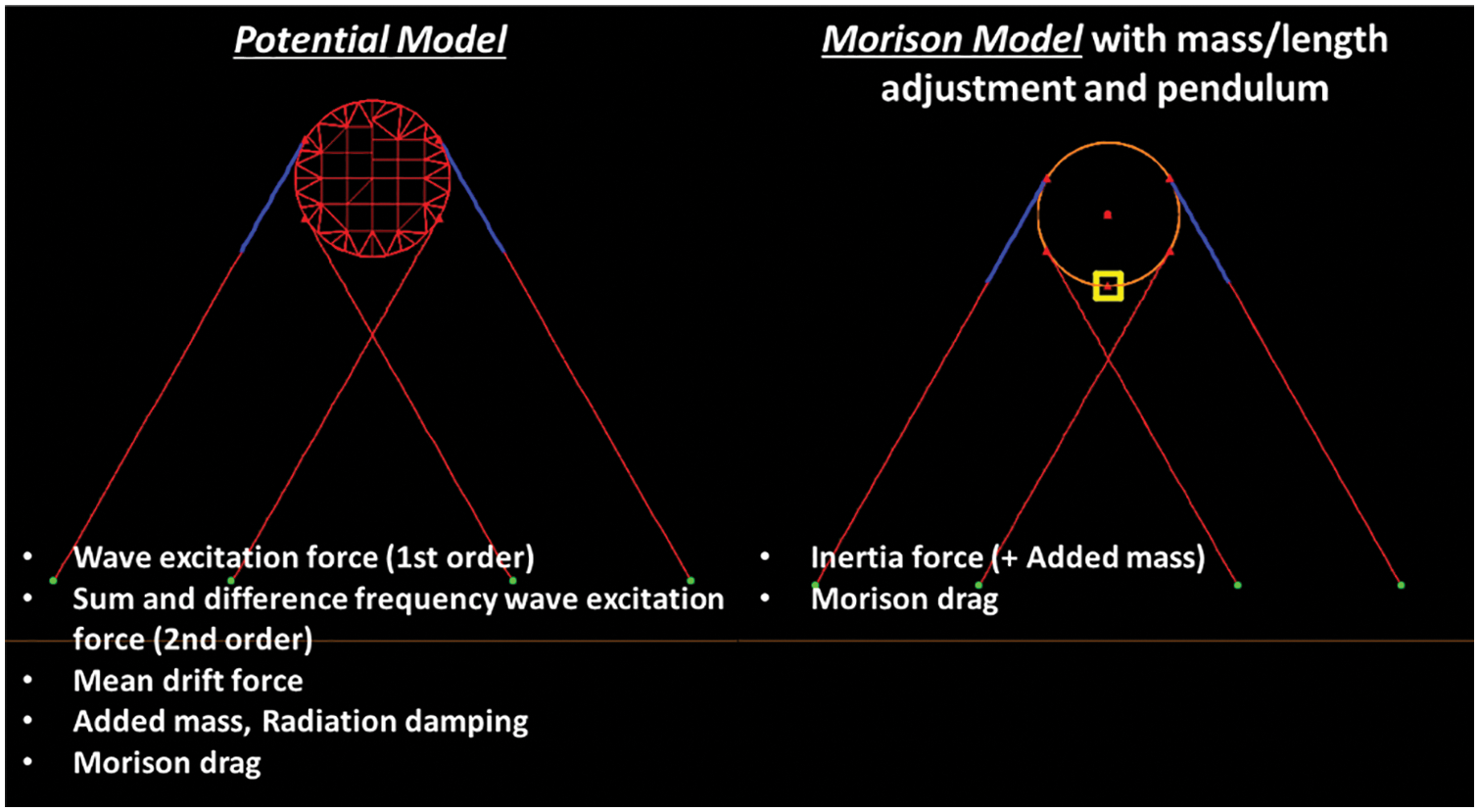
Figure 4: Configuration for dynamic response comparison between potential and Morison models

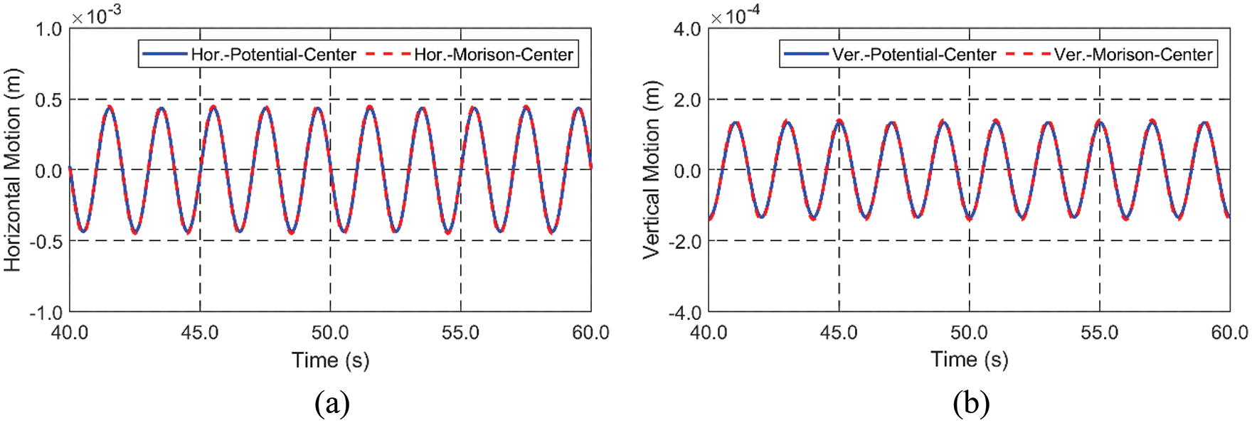
Figure 5: Time histories of horizontal (a) and vertical (b) motions between potential and Morison approaches, REG01

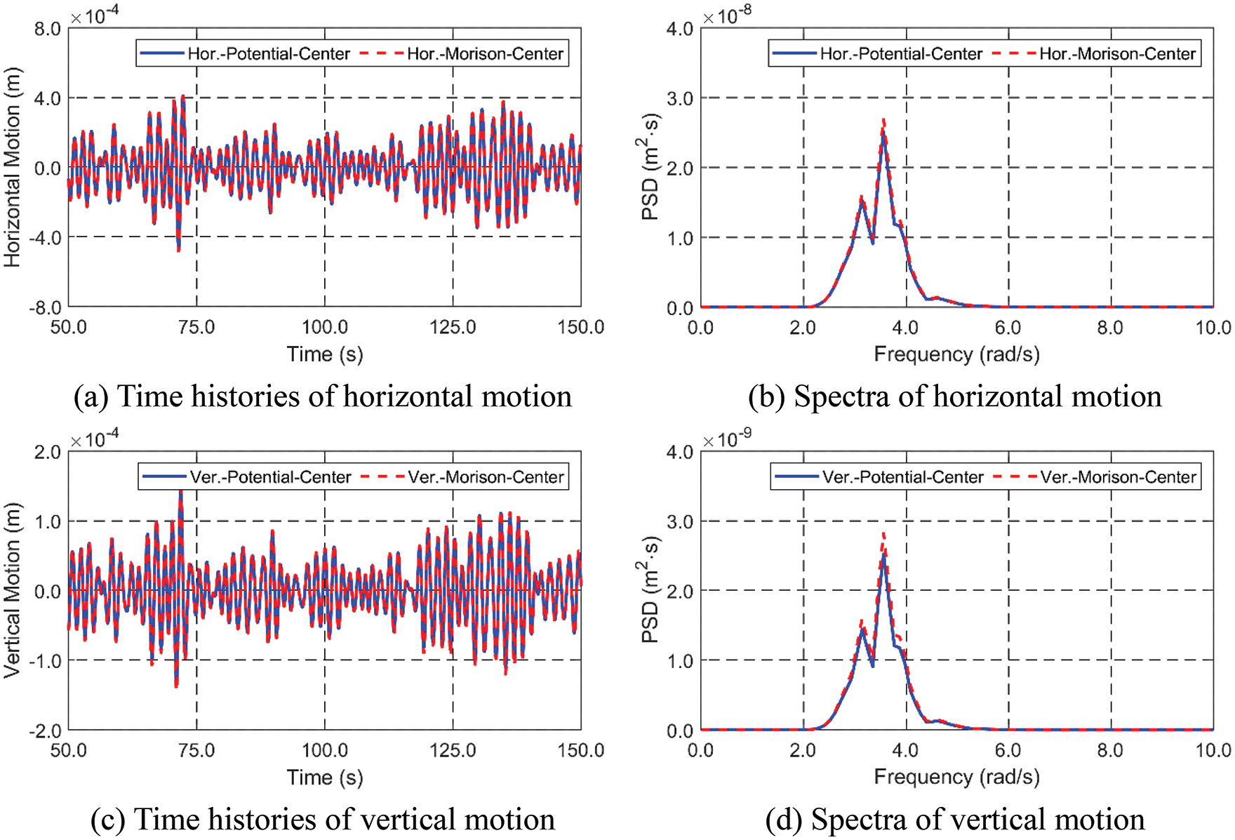
Figure 6: Time histories (a and c) and spectra (b and d) of horizontal (a and b) and vertical (c and d) motions between potential and Morison approaches, IRREG01

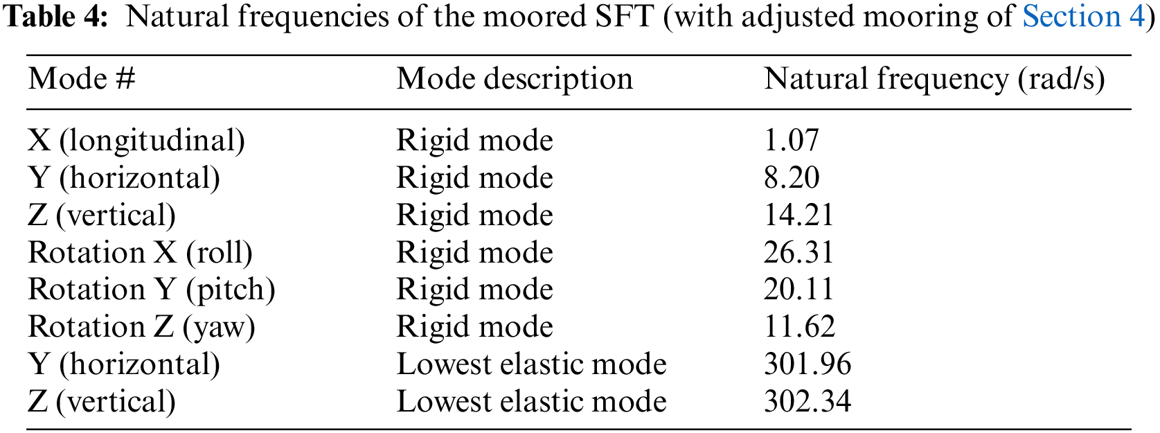
Next, let us consider the present moored SFT’s natural frequencies and natural modes, which are summarized in Table 4. The first six rows are natural frequencies for 6 degrees of freedom (DOF) rigid-body motions, and the last two rows are those for the lowest elastic modes. In the case of incident-wave angle normal to the longitudinal axis of SFT like the present case, only sway and heave rigid-body motions matter. Their natural frequencies are 8.2 and 14.2 rad/s, respectively. The heave mode is stiffer than the sway mode due to the 60-degree mooring inclination angle. Their natural frequencies are much higher than the range of incident-wave frequencies, and thus the relevant resonances are not likely to occur, as also shown in the following experimental and numerical results. Yaw and pitch motions are to be very small due to symmetry. In regard to elastic modes, the tunnel is rigid enough not to allow any appreciable elastic motions in view of very high lowest-elastic-wet-mode natural frequencies.

4  Forensic Analysis and Adjustment of Numerical Model

4.1 Mooring Line (ML) Length Adjustment for Pre-Tension Setup

In Section 3, it is confirmed that the Morison equation is sufficient to represent its global performance compared with the Cummins equation with 3D frequency-domain potential theory. In this regard, further simulations for comparing with experiments are only completed by the Morison-equation-based model. In this section, various adjustments of the numerical model are explained to have better similarities to the experimental model.

Due to the difficulty in the accurate length, assembly, and arrangement of the mooring system, there are mooring pre-tension (tension is abbreviated as TSN in figures) imbalances after submergence at the target distance. As shown in Fig. 7, the measured pre-tensions of mooring lines for the experimental model are different from those of the initial numerical model. In the numerical pre-tension, the pattern is symmetric with respect to the mid-length, as expected, but it is not so in the experimental setup. As for the experiment of typical moored floating offshore platforms, buoyancy is about the same as weight and initial mooring tension is small and their differences among lines are less important. Compared to the experiments of typical moored platforms, this SFT’s buoyancy is 1.3 times larger than weight, and thus very small differences in line lengths and toe angles result in nontrivial differences in initial tensions among lines. Therefore, perfect symmetry in experimental setup is hard to be achieved. This phenomenon is typical even in small-scale SFT experiment [35]. Thus, to make a similar condition to the experiment in the numerical model, an iterative line-length adjustment procedure for each line is implemented (Fig. 8). At each iteration, the differences in pre-tensions between the experiment and numerical model (ΔTSN) are calculated to slightly adjust the line length of each mooring line (Δδ) compared to the previous mooring length (L). The iteration process is repeated until the maximum difference in mooring tensions is within 10%. Fig. 9 represents the final comparison result after length adjustment. The general trends are similar, and the maximum pre-tension difference is 9.33% on ML03. After this kind of adjustment, the initial mooring line setup between the experiment and simulation becomes close to each other. Each mooring length after pre-tension adjustment is tabulated in Table 5. However, the subsequent comparisons of SFT horizontal and vertical motions measured from the experiment show significant differences compared to those by the numerical simulations in a regular wave (REG01) condition, as shown in Fig. 10. This led to further forensic analysis related to Young’s modulus adjustment, as explained in the following section.

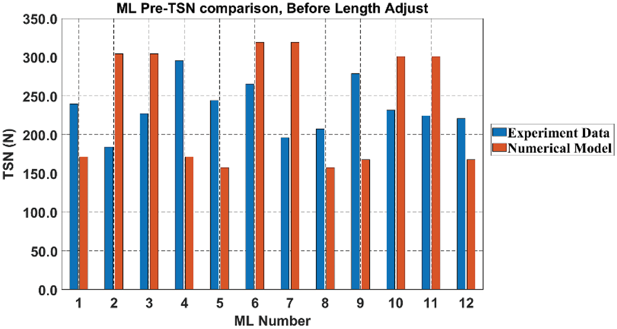
Figure 7: ML pre-tension comparison before length adjustment (original Young’s modulus)

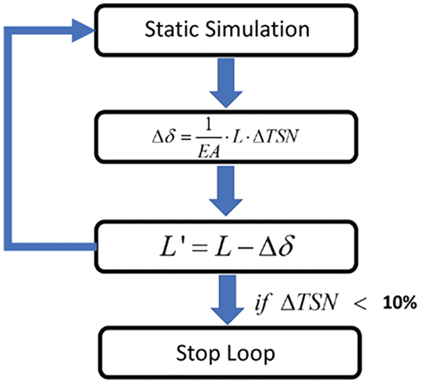
Figure 8: ML length adjustment for pre-tension set-up flow chart

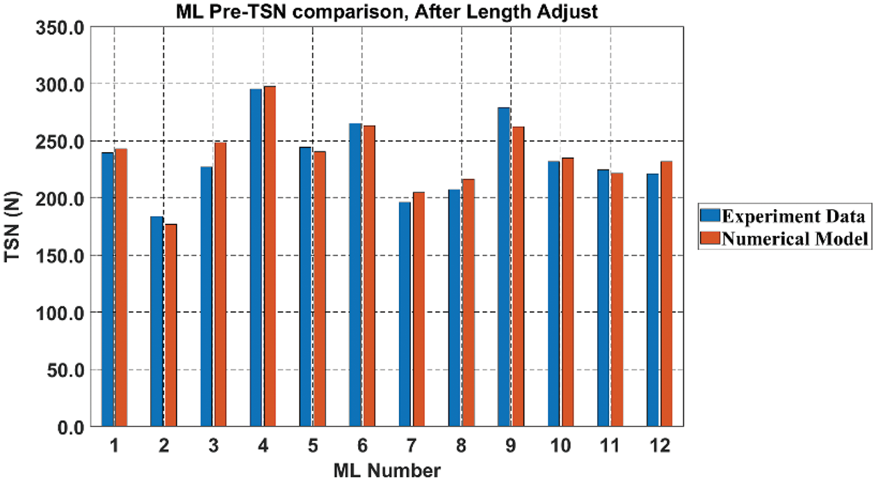
Figure 9: ML pre-tension comparison after length adjustment (original Young’s modulus)

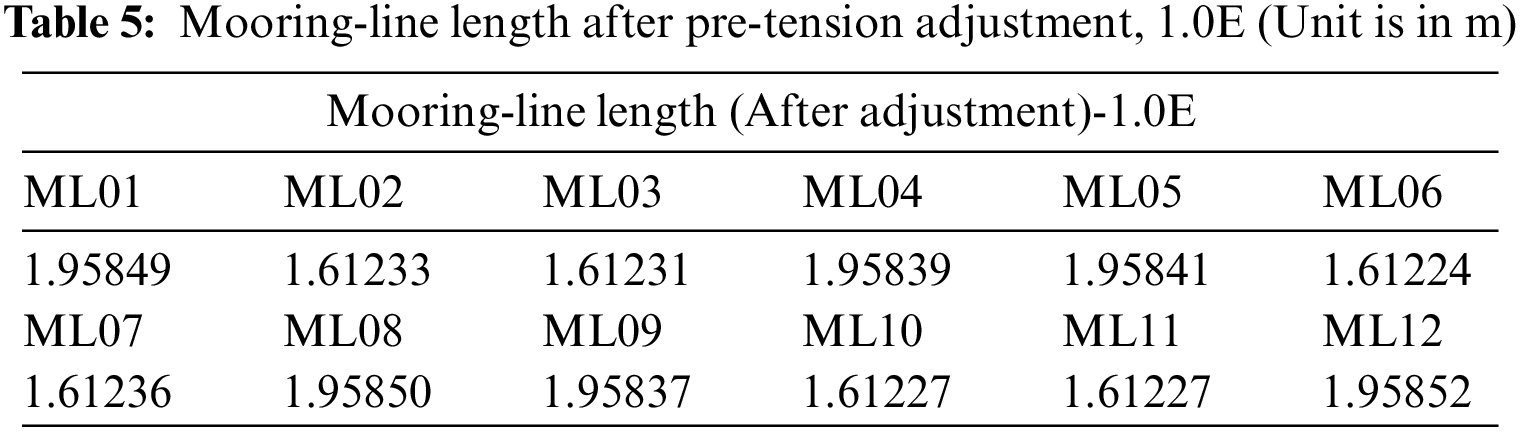
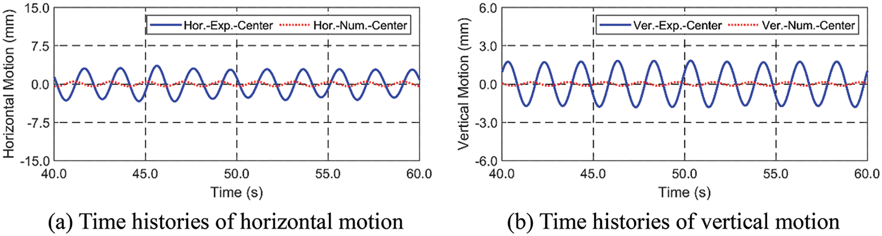
Figure 10: Comparison of horizontal (a) and vertical (b) motions between experiment vs. simulation (REG01)

4.2 Adjustment of Young’s Modulus of Mooring Line (Elastic to Plastic)

Due to the significant differences in measured and simulated dynamic responses, as observed in Fig. 10, the effect of Young’s modulus (E) of the mooring line, which characterizes the stiffness of mooring system, is additionally investigated to reduce the discrepancy between experiment and simulation as presented in this section. As shown in Fig. 11, Young’s modulus of aluminum is significantly changed if a certain elongation range is exceeded [36]. In this SFT experiment, the tendon-like aluminum tube is used as a mooring system in preference to typical mooring lines for several sensor-instrumentation purposes. Its joint to the SFT is more complex than typical hinged joints, and thus the joint also caused additional bending stresses on top of tensions at the fairlead position of the aluminum tube. Therefore, after the initial assembly of mooring system and installation at the target submergence depth, a fairly large strain (pre-strain data (right after being submerged) of ML02 and ML03 is 0.0157 and 0.01774) close to the plastic region (Fig. 11) was recorded. Subsequently, Young’s modulus of aluminum appeared to be changed from the elastic range to the plastic region. In this regard, we reset the Young’s-modulus to be 0.11E, which is close to that of aluminum in the plastic region as given by Merayo Fernández et al. [36]. Afterward, the iterative line-length-adjustment (Fig. 8) algorithm is utilized again (Table 6 shows the mooring line length after the iteration process), and the corresponding result of Fig. 12 is obtained. It is seen that the measured tension distribution can also be reproduced with the modified E value in the plastic region. The maximum difference between the experiment and simulation in this case is 9.41% on ML03. Actually, after several regular and irregular wave tests, the mooring system was broken, which indirectly shows that those mooring lines are close to the plastic region. After this kind of forensic analysis and adjustment of mooring system, comparisons between the measurement and simulation were made as follows.

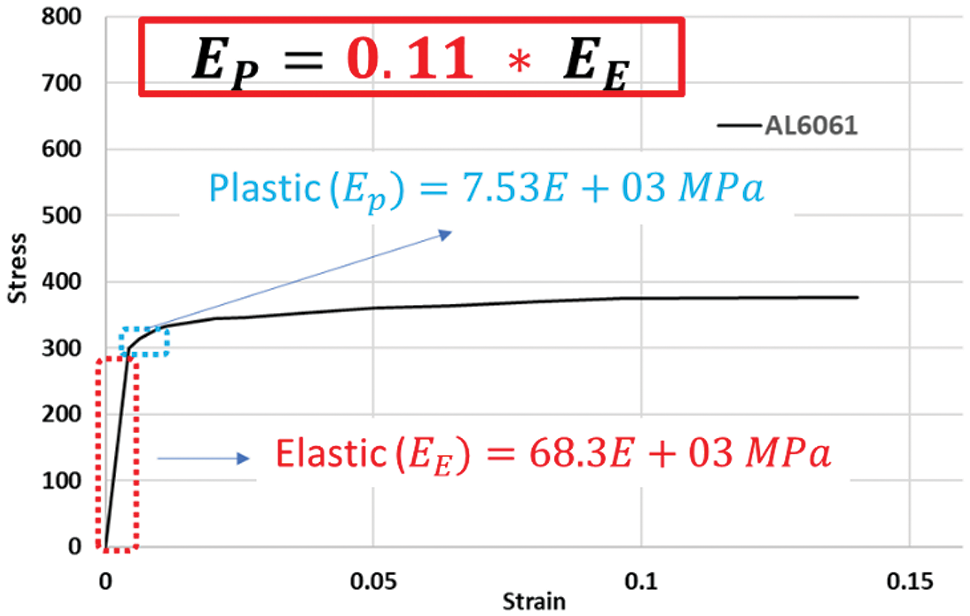
Figure 11: Aluminum modulus of elasticity adjustment [36], 0.11E

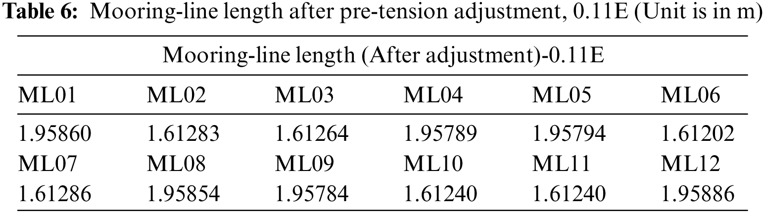
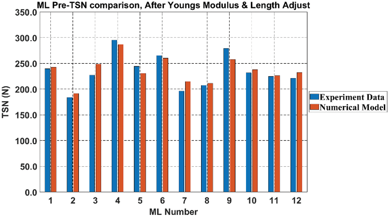
Figure 12: ML pre-tension comparison with modified Young’s modulus of 0.11 E

5  Comparisons between Experimental and Numerical Results

In this section, comparison results between the present experiment and simulation with modified Young’s modulus under regular and random waves are presented and discussed. The wave elevation for regular waves is generated in the numerical simulation at the same location of WAVE03 in Fig. 3, as shown in Fig. 13. It is confirmed that the same wave elevations are used in both physical experiment and numerical simulation. The wave crest line is parallel with the SFT, i.e., the wave propagating direction is perpendicular to the longitudinal axis of the tunnel. The corresponding time histories of horizontal and vertical responses are compared, as presented in Fig. 14. As it is shown, the horizontal dynamic responses are larger than vertical motions both in experiment and simulation. This is mainly due to the 60° mooring inclination angle, which produces larger mooring stiffness in the vertical direction. In the vertical responses, both experiment and simulation show larger downward-motion amplitudes than upward-motion amplitudes. Mooring tensions are further compared in Fig. 15. Since it is found that strain gages on ML02 and ML03 are the most reliable, the measured tensions at ML02 and ML03 are compared against the corresponding simulated tensions. Similar trends in tension magnitudes can be observed both in experiment and simulation. In the REG02 case, the measured mooring line tension can be negative (compression), but the simulated one remains zero after being slightly slack. Due to this weaker vertical stiffness in the downward direction, the downward vertical response becomes larger than the upward one, as mentioned above. From the simultaneous coincidence of motions and tensions between the experiment and simulation, the adjustments done in the numerical line modeling seem reasonable.

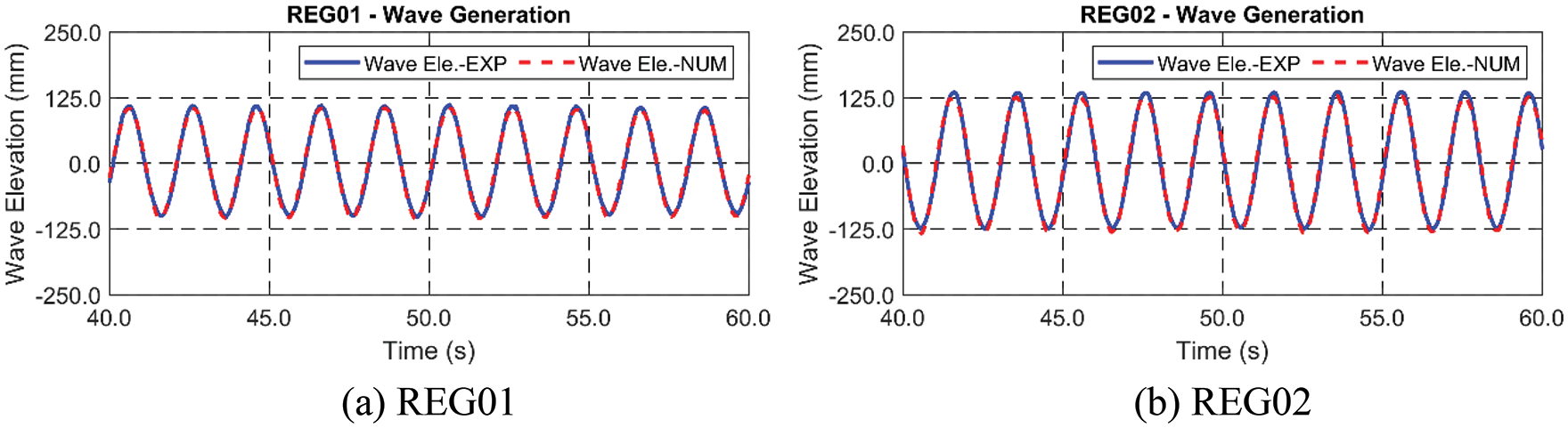
Figure 13: Times histories of wave elevations between experiment and simulation under regular wave excitations

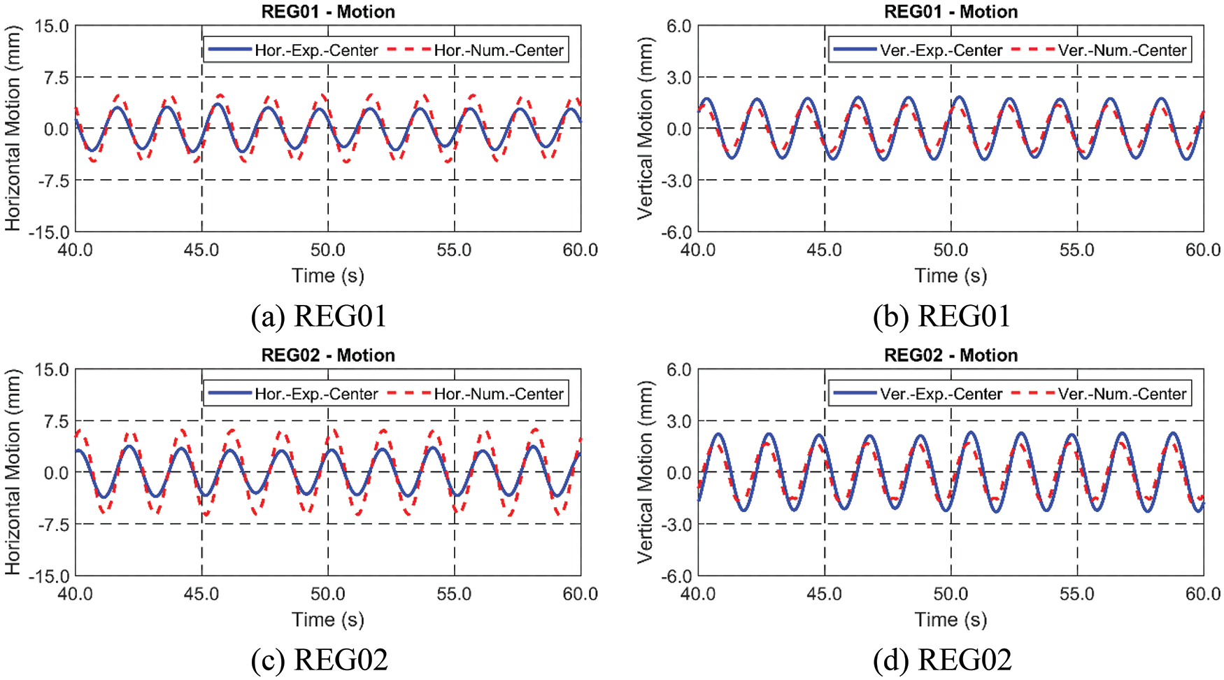
Figure 14: Times histories of horizontal (a and c) and vertical (b and d) responses between experiment and simulation under regular wave excitations

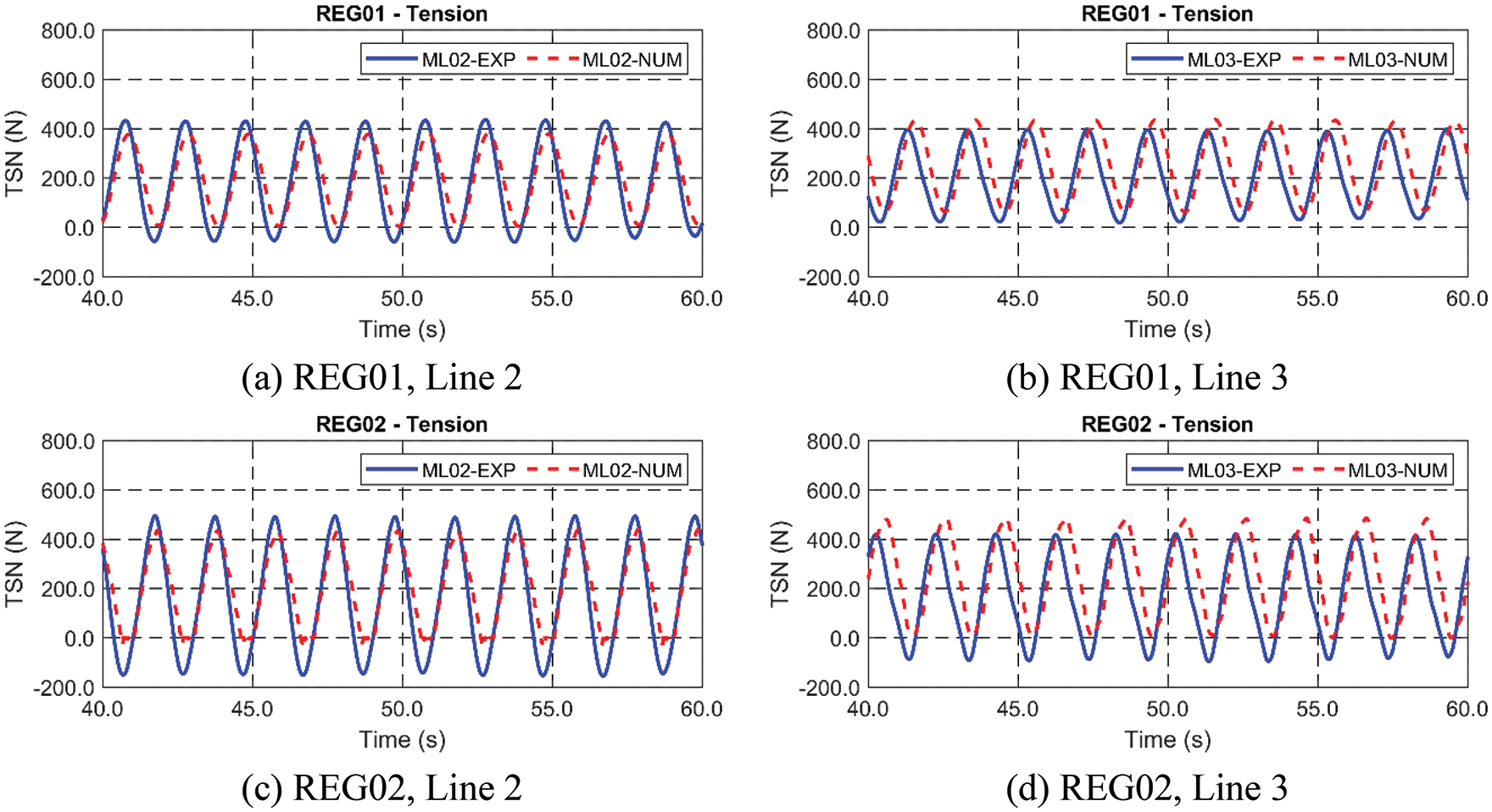
Figure 15: Times histories of mooring tensions between experiment and simulation under regular wave excitations

Next, an irregular wave case is presented. At first, to confirm that the same irregular wave condition is inputted into the experiment and simulation, the two wave time histories and spectra are compared in Fig. 16. For this comparison, the measured time history in the experiment is inputted to simulation through the use of FFT (fast Fourier transform) and the corresponding component wave amplitudes and phases. The compared time histories and PSDs (Power Spectral Densities) are almost identical, which means that the similarity of the wave condition to each physical and numerical system is confirmed in the irregular-wave case. The inputted Hs and Tp are 0.2 m and 1.73 s (= 3.6 rad/s), which corresponds well with the experimental and numerically reproduced waves. The corresponding motion time histories and PSDs are plotted in Fig. 17. The first peak (3.56 rad/s) related to the wave frequency can be observed in both experiment and simulation regardless of motion direction. However, there are additional second (4.71 rad/s) and third (5.45 rad/s) minor peaks only in the horizontal motion of the experiment, whereas no such minor peaks are present in the simulation. Such minor peaks at the same locations are also seen in the input wave spectrum to a lesser degree. Earlier comparisons in Fig. 6 and Table 4 indicate that it is not likely from the hydro-elasticity or second-order wave effects. It is not from the nonlinear viscous drag force either since the relevant KC (Keulegan Carpenter) number is small (around 1, so inertia force dominant), and thus the drag force only plays a very minor role. Instead, subtle nonlinear coupling associated with the physical mooring assembly and the observed nontrivial cylinder rotation may be involved. The reflected waves from tank walls in the experiment, although they are small, may also be relevant. Similar to the regular wave cases, horizontal motions in the numerical simulation are overestimated, while the reverse trend is seen in the vertical motion. Furthermore, tension comparison results are presented in Fig. 18. The PSD of ML02 tension is almost identical, while there is a little reduction in the peak frequency in ML03. Judging from the comparisons between the experimental and numerical results, the physical system is reasonably modeled by the present simulation program so that it can be repeatedly used for other cases.

Figure 16: Time histories (a) and spectra (b) of random waves between experiment and simulation

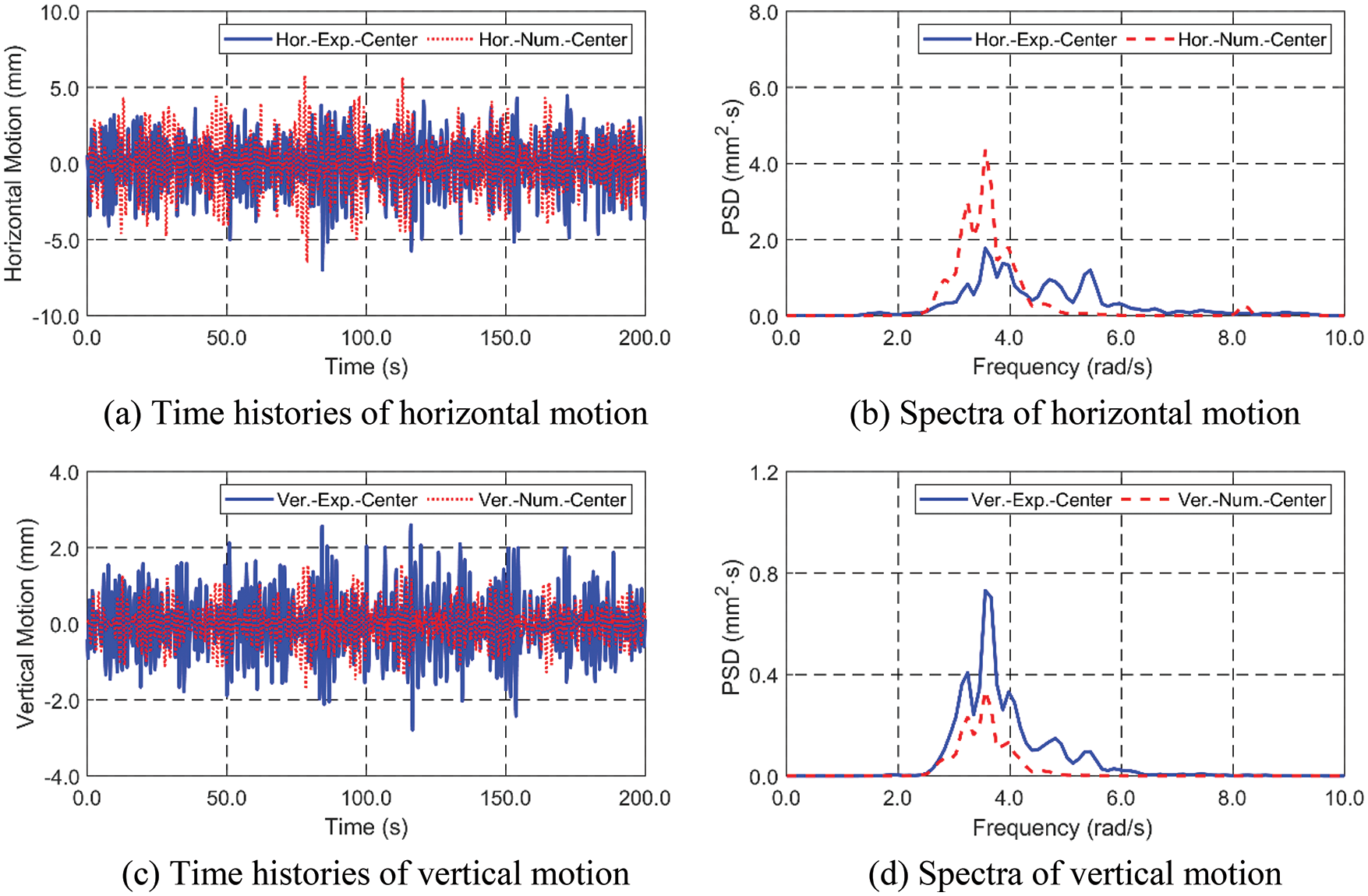
Figure 17: Time histories (a and c) and spectra (b and d) of horizontal (a–b) and vertical (c–d) motions between experiment and simulation under random waves

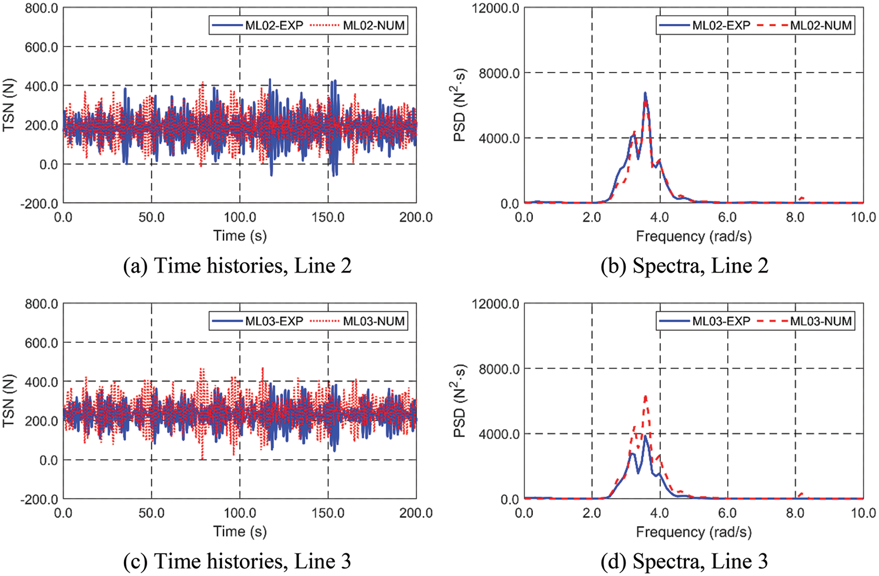
Figure 18: Time histories (a and c) and spectra (b and d) of mooring tensions between experiment and simulation under random waves

To check the sensitivity of the wave-induced-force with respect to the drag coefficient Cd in the numerical model, two results with Cd = 0.55 and 2.0 are compared in Fig. 19. As pointed out in the previous discussion, since the KC number is near 1, the viscous drag force plays a very minor role. Finally, static offset tests were conducted to characterize the system stiffness by using the numerical simulation program. The static offset tests were carried out after the static equilibrium of the whole system was reached. Horizontal and vertical static forces were plotted for the increment of horizontal and vertical static displacements, as shown in Fig. 20. Due to the 60-deg toe angle of the mooring lines, the vertical stiffness is about twice larger than the horizontal stiffness, which is also well matched against the calculated wet natural frequencies in Table 4. This is why the maximum horizontal-motion amplitude is about twice the maximum vertical-motion amplitude in Fig. 17.

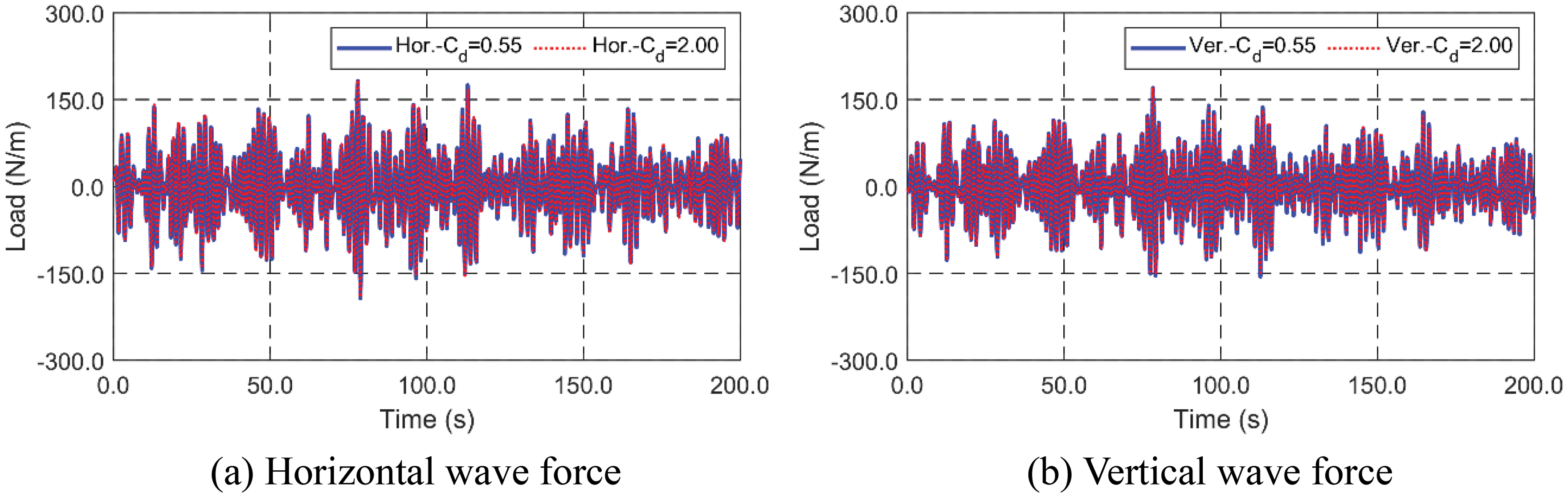
Figure 19: Time histories of horizontal (a) and vertical (b) wave forces per unit length of the cylinder with Cd = 0.55 and 2.0

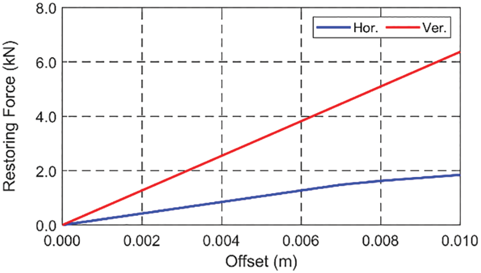
Figure 20: Numerical static offset test to find horizontal and vertical stiffness of the SFT system

6  Conclusions

In this paper, a comparative study between experiment and simulation for a SFT was conducted under regular and random waves. The related forensic analysis for mooring system modeling and failure was also presented. The experiments were conducted in the KRISO 3D wave tank with 1:33.3-scale, and the results were compared with the numerical results from the coupled-dynamic time-domain simulations. The tunnel and mooring lines were made of concrete and aluminum hollow tubes, respectively. Two numerical models, which are the Cummins equation with 3D potential theory, including second-order diffraction/radiation effects and the simpler Morison-equation-based formulation, were first compared. The two methods agreed well, so the Morison-based approach was used for later comparisons. The physical mooring-line assembly and set-up were rather complicated, and two reasonable mooring-line forensic adjustments (iterative line-length adjustment and axial stiffness adjustment) were conducted to reproduce the measured properties of the physical mooring system. After that, the measured and simulated dynamic responses and mooring tensions of the SFT were compared under regular and irregular waves. Considering the complex setup of the whole system, the measured and simulated results compared reasonably well for both regular- and irregular-wave conditions. The reproduced system characteristics also coincided with the measured results. This means that the developed methodology and simulation tool can reasonably represent the actual dynamic behaviors of the SFT and thus can repeatedly be used with varying design parameters to find the optimal design for any given environmental conditions.

Funding Statement: This work was supported by the National Research Foundation of Korea (NRF) grant funded by the Korea Government (MSIT) (No. 2017R1A5A1014883).

Conflicts of Interest: The authors declare that they have no conflicts of interest to report regarding the present study.

References

1. Faggiano, B., Landolfo, R., Mazzolani, F. (2005). The SFT: An innovative solution for waterway strait crossings. IABSE Symposium, pp. 36–42. Lisbon, Portugal. [Google Scholar]

2. Remseth, S., Leira, B. J., Okstad, K. M., Mathisen, K. M., Haukås, T. (1999). Dynamic response and fluid/structure interaction of submerged floating tunnels. Computers & Structures, 72(4–5), 659–685. https://doi.org/10.1016/S0045-7949(98)00329-0 [Google Scholar] [CrossRef]

3. Faggiano, B., Landolfo, R., Mazzolani, F. M. (2001). Design and modelling aspects concerning the submerged floating tunnels: An application to the messina strait crossing. Krobeborg. Strait Crossing, 511–519. [Google Scholar]

4. Lu, W., Ge, F., Wang, L., Wu, X., Hong, Y. (2011). On the slack phenomena and snap force in tethers of submerged floating tunnels under wave conditions. Marine Structures, 24(4), 358–376. https://doi.org/10.1016/j.marstruc.2011.05.003 [Google Scholar] [CrossRef]

5. Martinelli, L., Barbella, G., Feriani, A. (2011). A numerical procedure for simulating the multi-support seismic response of submerged floating tunnels anchored by cables. Engineering Structures, 33(10), 2850–2860. https://doi.org/10.1016/j.engstruct.2011.06.009 [Google Scholar] [CrossRef]

6. Won, D., Seo, J., Kim, S., Park, W. S. (2019). Hydrodynamic behavior of submerged floating tunnels with suspension cables and towers under irregular waves. Applied Sciences, 9(24), 5494. https://doi.org/10.3390/app9245494 [Google Scholar] [CrossRef]

7. Jin, C., Kim, M. H. (2018). Time-domain hydro-elastic analysis of a SFT (submerged floating tunnel) with mooring lines under extreme wave and seismic excitations. Applied Sciences, 8(12), 2386. https://doi.org/10.3390/app8122386 [Google Scholar] [CrossRef]

8. Kunisu, H., Mizuno, S., Mizuno, Y., Saeki, H. (1994). Study on submerged floating tunnel characteristics under the wave condition. The Fourth International Offshore and Polar Engineering Conference, pp. 27–32. Osaka, Japan. [Google Scholar]

9. Kunisu, H. (2010). Evaluation of wave force acting on submerged floating tunnels. Procedia Engineering, 4, 99–105. https://doi.org/10.1016/j.proeng.2010.08.012 [Google Scholar] [CrossRef]

10. Oh, S. H., Park, W. S., Jang, S. C., Kim, D. H. (2013). Investigation on the behavioral and hydrodynamic characteristics of submerged floating tunnel based on regular wave experiments. Journal of the Korean Society of Civil Engineers, 33(5), 1887–1895. https://doi.org/10.12652/Ksce.2013.33.5.1887 [Google Scholar] [CrossRef]

11. Seo, S. I., Mun, H. S., Lee, J. H., Kim, J. H. (2015). Simplified analysis for estimation of the behavior of a submerged floating tunnel in waves and experimental verification. Marine Structures, 44, 142–158. https://doi.org/10.1016/j.marstruc.2015.09.002 [Google Scholar] [CrossRef]

12. Li, Q., Jiang, S., Chen, X. (2018). Experiment on pressure characteristics of submerged floating tunnel with different section types under wave condition. Polish Maritime Research, 25, 54–60. https://doi.org/10.2478/pomr-2018-0112 [Google Scholar] [CrossRef]

13. Yang, Z., Li, J., Zhang, H., Yuan, C., Yang, H. (2020). Experimental study on 2D motion characteristics of submerged floating tunnel in waves. Journal of Marine Science and Engineering, 8(2), 123. https://doi.org/10.3390/jmse8020123 [Google Scholar] [CrossRef]

14. Deng, S., Ren, H., Xu, Y., Fu, S., Moan, T. et al. (2020). Experimental study of vortex-induced vibration of a twin-tube submerged floating tunnel segment model. Journal of Fluids and Structures, 94, 102908. https://doi.org/10.1016/j.jfluidstructs.2020.102908 [Google Scholar] [CrossRef]

15. Deng, S., Ren, H., Xu, Y., Fu, S., Moan, T. et al. (2020). Experimental study on the drag forces on a twin-tube submerged floating tunnel segment model in current. Applied Ocean Research, 104, 102326. https://doi.org/10.1016/j.apor.2020.102326 [Google Scholar] [CrossRef]

16. Xiang, Y., Chen, Z., Bai, B., Lin, H., Yang, Y. (2020). Mechanical behaviors and experimental study of submerged floating tunnel subjected to local anchor-cable failure. Engineering Structures, 212, 110521. https://doi.org/10.1016/j.engstruct.2020.110521 [Google Scholar] [CrossRef]

17. Xiang, Y., Lin, H., Bai, B., Chen, Z., Yang, Y. (2021). Numerical simulation and experimental study of submerged floating tunnel subjected to moving vehicle load. Ocean Engineering, 235, 109431. https://doi.org/10.1016/j.oceaneng.2021.109431 [Google Scholar] [CrossRef]

18. Won, D., Seo, J., Park, W. S., Kim, S. (2021). Torsional behavior of precast segment module joints for a submerged floating tunnels. Ocean Engineering, 220, 108490. https://doi.org/10.1016/j.oceaneng.2020.108490 [Google Scholar] [CrossRef]

19. Cifuentes, C., Kim, S., Kim, M. H., Park, W. S. (2015). Numerical simulation of the coupled dynamic response of a submerged floating tunnel with mooring lines in regular waves. Ocean Systems Engineering, 5(2), 109–123. https://doi.org/10.12989/ose.2015.5.2.109 [Google Scholar] [CrossRef]

20. Lee, J. Y., Jin, C., Kim, M. (2017). Dynamic response analysis of submerged floating tunnels by wave and seismic excitations. Ocean Systems Engineering, 7(1), 1–19. https://doi.org/10.12989/ose.2017.7.1.001 [Google Scholar] [CrossRef]

21. Jin, R., Gou, Y., Geng, B., Zhang, H., Liu, Y. (2020). Coupled dynamic analysis for wave action on a tension leg-type submerged floating tunnel in time domain. Ocean Engineering, 212, 107600. https://doi.org/10.1016/j.oceaneng.2020.107600 [Google Scholar] [CrossRef]

22. Chen, X., Chen, Q., Chen, Z., Cai, S., Zhuo, X. et al. (2021). Numerical modeling of the interaction between submerged floating tunnel and surface waves. Ocean Engineering, 220, 108494. https://doi.org/10.1016/j.oceaneng.2020.108494 [Google Scholar] [CrossRef]

23. Jin, C., Kim, M. (2021). The effect of key design parameters on the global performance of submerged floating tunnel under target wave and earthquake excitations. Computer Modeling in Engineering & Sciences, 128(1), 315–337. https://doi.org/10.32604/cmes.2021.016494 [Google Scholar] [CrossRef]

24. Jin, C., Kim, M. H. (2020). Tunnel-mooring-train coupled dynamic analysis for submerged floating tunnel under wave excitations. Applied Ocean Research, 94, 102008. https://doi.org/10.1016/j.apor.2019.102008 [Google Scholar] [CrossRef]

25. Orcina, Ltd. (2018). OrcaFlex manual. Daltongate Ulterston Cumbria, UK. [Google Scholar]

26. Morison, J. R., Johnson, J. W., Schaaf, S. A. (1950). The force exerted by surface waves on piles. Journal of Petroleum Technology, 2(5), 149–154. https://doi.org/10.2118/950149-G [Google Scholar] [CrossRef]

27. Jin, C., Kim, G. J., Kim, S. J., Kim, M., Kwak, H. G. (2023). Discrete-module-beam-based hydro-elasticity simulations for moored submerged floating tunnel under regular and random wave excitations. Engineering Structures, 275, 115198. https://doi.org/10.1016/j.engstruct.2022.115198 [Google Scholar] [CrossRef]

28. Kim, M. H., Yue, D. K. (1991). Sum- and difference-frequency wave loads on a body in unidirectional Gaussian seas. Journal of Ship Research, 35(2), 127–140. https://doi.org/10.5957/jsr.1991.35.2.127 [Google Scholar] [CrossRef]

29. Lee, C. H. (1995). WAMIT theory manual. Massachusetts Institute of Technology. [Google Scholar]

30. Cummins, W. E., Iiuhl, W., Uinm, A. (1962). The impulse response function and ship motions. The Symposium on Ship Theory, pp. 1–9. Hamburg, Germany. [Google Scholar]

31. Lawson, T., Anthony, K., Cockrell, D., Davenport, A., Flint, A. et al. (1986). Mean forces, pressures and flow field velocities for circular cylindrical structures: Single cylinder with two-dimensional flow. Engineering Sciences Data Unit (ESDU), 80025, 1–66. [Google Scholar]

32. Jin, C., Kim, M. (2017). Dynamic and structural responses of a submerged floating tunnel under extreme wave conditions. Ocean Systems Engineering, 7(4), 413–433. [Google Scholar]

33. Faltinsen, O. (1993). Sea loads on ships and offshore structures. London, UK: Cambridge University Press. [Google Scholar]

34. Kim, M. H., Yue, D. K. (1989). The complete second-order diffraction solution for an axisymmetric body Part 1. monochromatic incident waves. Journal of Fluid Mechanics, 200, 235–264. https://doi.org/10.1017/S0022112089000649 [Google Scholar] [CrossRef]

35. Kim, G. J., Lee, S., Kim, M., Kwak, H. G., Hong, J. W. (2022). Characterization of single and dual SFT through a hydraulic experiment under regular and irregular waves. Ocean Engineering, 263, 112365. https://doi.org/10.1016/j.oceaneng.2022.112365 [Google Scholar] [CrossRef]

36. Merayo Fernández, D., Rodríguez-Prieto, A., Camacho, A. M. (2020). Prediction of the bilinear stress-strain curve of aluminum alloys using artificial intelligence and big data. Metals, 10(7), 904. https://doi.org/10.3390/met10070904 [Google Scholar] [CrossRef]