Physics-Informed AI Surrogates for Day-Ahead Wind Power Probabilistic Forecasting with Incomplete Data for Smart Grid in Smart Cities

Nomenclature

1  Introduction

As renewable energy like wind, photovoltaic and tidal power are increasingly incorporated into smart grids, the stochastic and uncertainty features of which brought additional challenges to the electricity market and energy system [1,2]. Wind power, the most popular renewable energy, is highly fluctuating, making accurate wind power forecasting critical in planning and managing energy systems with wind farms [3]. Various forecasting temporal, horizons exist, from long-term (longer than 1 day) to very short-term (within 1 h) for specific management tasks in smart grids and buildings approaches [4]. Among these, the high-resolution (10∼15 min interval) day-ahead probabilistic forecasting can provide meaningful uncertainty quantification information [5], which is valuable in the reliability/resilience modeling and analysis [6,7] for daily operating, controlling, and scheduling maintenance of smart grids. Thus, it has become one of the latest key research areas in smart and sustainable cities [8].

There are two main difficulties in day-ahead probability forecasting of wind power. First, unlike conventional power plants, many wind farms, especially the smart wind grids around smart cities, are newly built, with limited historical power generation data [9], and second, the operation of wind farms is highly flexible due to the fluctuating wind speed, which means occasional power adjustment or shutdown [10]. The above difficulties can be summarized as an incomplete dataset with insufficient data, missing data, and several outliers, which constrained the generalization ability of the forecasting model trained on it.

Two kinds of improved forecasting approaches can be conducted to tackle the generalization difficulty: physics-based and data-driven methods [11,12]. Computationally intensive physics-based methods are more appropriate for long-term forecasting due to their low efficiency and ability to simulate seasonal and chaotic weather factors. Data-driven methods mainly learn the trend of wind speed and wind power through autoregression algorithms, which have a non-ignorable shortcoming: the forecasting process should be a continuous iteration of prior and posterior data points, so it is difficult to handle the shutdown situation, i.e., data missing.

Physics-informed neural networks (PINN) were first named by Raissi et al. [13] as a key to joining physical laws into machine learning to enhance the networks’ ability to solve a high-dimensional problem with limited training samples [14]. In the broad sense, PINN can also be seen as a neural network method based on information fusion, except that it fuses physical information [15]. In the broad sense, PINN can also be seen as a neural network method that fuses physical information to improve its training efficiency and generalization ability. Hence, enlightened by the idea of PINN, using physics information such as NWP data to improve the data-driven wind power forecasting model making it more suitable for incomplete datasets, is promising.

Informed by the literature review (See Section 2), this paper presents a probabilistic forecasting method based on physics-informed AI surrogates, a regression approach that fused physics information into the AI-based forecasting method. Two AI surrogates were built under a Bayesian network structure. The first surrogate fuses the physics information in raw NWP data and transforms it into selected factors (SF) highly related to wind power. The second surrogate acts as the response surface of SFs to wind power generation. The quality of the surrogates’ training set is improved by comprehensively leveraging the generative adversarial network (GAN) based data augmentation methods [16] and K-means cluster-based resampling. Therefore, the proposed method can provide reliable day-ahead probabilistic wind power forecasting with an incomplete dataset. The paper details how:

1.    A multiple AI surrogates regression structure for day-ahead wind power probabilistic forecasting with an incomplete dataset, which infused the physics information from NWP and weather monitoring data to enhance forecasting accuracy was built.

2.    A data augmentation method based on two kinds of GAN corresponding to the multi-surrogate model, improving the model’s generalization ability, and supporting quantifying the uncertainty propagation was created.

3.    The proposed method’s forecasting and uncertainty quantification abilities were benchmarked by applying it to a real case dataset from a wind farm together with conventional methods.

The rest of this paper is organized as follows. Section 2 provides the background knowledge used in this paper. Section 3 delivers the workflow of the proposed multi-surrogate method. The application procedure with a real wind farm case is delivered in Section 4, together with the discussion to compare with other methods. Section 5 summarizes this paper.

2  Related Works

2.1 Wind Power Forecasting Methods

The uncertainty of wind power generation has many aspects, from stochastic weather factors to inconsistent efficiency of wind turbines. Research works for wind power forecasting can be classified through the materials that are used to quantify the uncertainty: the regression methods based on physics information from NWP data or simulation and the autoregression method based on monitored wind speed and power data.

Physics-based methods are generally powered by numerical weather prediction (NWP) data and computational fluid dynamics (CFD) simulation. Che et al. [17] introduced a multiscale model for day-ahead wind speed forecasting, which conducted a joint simulation of mesoscale weather research forecasting (WRF) and microscale CFD models for a specific wind farm, significantly improving the wind speed prediction accuracy. Cuevas-Figueroa et al. [18] discussed the accuracy of using the NWP and WRF to predict the wind farm operating performance and proved the confidence even in complex terrain. Zhang et al. [19] proposed a tensor-based method that combines Tucker decomposition and computational fluid dynamics (CFD) to reconstruct three-dimensional wind velocity distributions for short-term wind speed prediction. However, the scattered areas and complex terrain of wind farms cause the errors between day-ahead NWP and real near-surface weather factors may not be ignored. Due to NWP errors, there is a multiple-to-one mapping relationship between NWP data and wind power generation in the training dataset, making the generalization ability of the forecasting model trained on it may be constrained. Simply increasing the training sample size will not solve the problem.

Data-driven methods utilize statistical or artificial intelligence (AI) based models to predict future power generation with historical and online monitoring data [20,21]. These methods mainly focus on short-term data pattern analysis with decomposition [22], uncertainty inferencing [23], and data augmentation [24] techniques to tackle the limited and complex signals, which makes them more flexible and sensitive for minute or hourly trends. Based on direct quantile regression (DQR), Wan et al. [25] proposed a nonparametric probability forecasting method for wind power. The prediction performance proved reliable given the fast learning speed of extreme learning machines (ELM) and DQR’s nonparametric feature that bypassed distribution assumptions. Mehdi et al. [26] deployed a deep learning-based model for the forecasting of the power output in wind farms, which employs wind speed, wind direction, and current power output as model inputs. An adaptive variational mode decomposition (VMD) method and long short-term memory (LSTM) deep neural networks were combined as the predicting model. Victor et al. [27] proposed a Bayesian dynamical model for joint modeling the wind speed and wind power that account for temporal dependence, nonstationary behavior, and truncation of power due to turbine specifications. Boudy et al. [28] presented an adaptive neuro-fuzzy inference system modeling approach for wind turbine output power predicting, including the wind speed, turbine rotational speed, and mechanical-to-electrical power converter’s temperature as model inputs. Data-driven methods may achieve high predicting accuracy even in day-ahead forecasting scenarios. Nevertheless, its accuracy relies on data preprocessing to tackle the missing data and outliers and cannot directly handle the forecasting task after wind turbine rebooting.

Meanwhile, incorporating physical information and neural networks (NN) to enrich the generalization ability is also a growing field in wind power forecasting. Wu et al. [29] proposed a probabilistic forecasting method for wind power based on an adaptive neuro-fuzzy inference system and a fuzzy C-means clustering algorithm, which proved that ensemble NWP data could improve the performance of NN forecast models. A combined model was presented by He et al. [30], which leverages the mutual information to select the most representative NWP subset and then the K-means algorithm to group meteorological features to improve the generalization ability of a convolutional neural network and long short-term memory (CNN-LSTM) prediction model of wind power. Xia et al. [31] proposed a wind power ramping events prediction model powered by a classified spatiotemporal network that considered a resampled NWP dataset in which the rare extreme weather samples were augmented with a GAN. A short-term interval prediction method for wind speed was illustrated by Han et al. [32] using VMD to extract the time-series features of NWP data and to generate the prediction interval (PI) of wind speed using multivariate line regression and a GAN. Although, the physics-informed approaches above are all short-term (one-step or multi-step) methods that cannot maintain availability under day-ahead forecasting scenarios. However, these approaches did indicate that physics information can enrich the data-driven forecasting model through clustering, decomposing, or feature augmenting, without intensive computation, i.e., building a lightweight surrogate for physics information to inform the forecasting model is possible and valuable.

2.2 Extreme Learning Machine

An extreme learning machine is a single hidden layer feedforward neural network (SLFN) [33]. Without the feedback step, the hidden nodes’ parameters (weight and bias) will not evolve during learning. This simple structure makes ELM possess good generalization ability and more rapid learning than most other networks with backpropagation. Fig. 1 shows an ELM with one hidden layer of L nodes.

Figure 1: The structure of ELM

The output function of a single layer ELM with L nodes ni(x)=F(αi,βi,x) is:

fL(x)=∑i=1Lωini(x)(1)

where αi and βi are the function parameters, and ωi is the weight of the node. Given m training samples, the output matrix of ELM is:

N=[n(xi)⋮n(xm)]=[F(α1,β1,x1)⋯F(αL,βL,x1)⋮⋱⋮F(α1,β1,xm)⋯F(αL,βL,xm)](2)

where n(xi)=[ni(x),⋯,nL(x)]. Let the training target matrix I be Y=[y1⋯ym]T, then the optimized objective function of ELM can be written as:

||Nω^−I||=minβ||Nω−I||(3)

Owing to the high training speed and adaptability for non-linear activation functions, the ELM has been deterministically and probabilistically applied to wind speed and power forecasting [34].

2.3 Generative Adversarial Network

Since the GAN was first introduced in 2014 [35], it has been applied in a vast range of fields for data augmentation tasks [36]. Compared with other data augmentation methods such as Monte Carlo [37] and bootstrap [38], GAN-based methods do not need a pre-defined distribution and can handle extremely small datasets with the cost of some training time. GAN has gradually become one of the leading AI methods in data augmentation due to these advantages. In the wind power predicting field, Xia et al. [31] introduced GAN to augment rare extreme weather samples to improve the accuracy of ramping events. Different from the structure of the auto-encoder neural network [39], GAN is constructed with two adversarial deep learning NNs: the generator (net G) and the discriminator (net D). Through the adversarial training of nets G and D, GAN is capable in non-supervised or semi-supervised learning tasks of generating realistic synthetic data from arbitrary raw data.

The objective function of GAN has many forms, in which the Wasserstein distance based function (i.e., Earth–Mover distance), W(x,x~)=Ex∼Pr[D(x)]−Ex~∼Pg[D(x~)], is physics meaningful and continuous at the point 0 [40] the objective function of the Wasserstein GAN (WGAN) with gradient penalty is:

minGmaxDEx∼Pg[D(x)]−Ex~∼Pr[D(x~)]+Lgp(4)

where the distribution of original data is x∼Pr, the distribution of generated data is x~∼Pg. Lgp=λEx^∼Px^[(||∇x^D(x^)||2−1)2] is the gradient penalty term to improve the training stability with randomly sampled x^∼Px^ along straight lines between points sampled from Pr and Pg. λ is an adjustable training parameter [41]. The structure of WGAN is shown in Fig. 2. In practice, most monitored data have time-varying characters [42]. Based on the WGAN, our team has proposed an auto-augmentation algorithm for time-series data called worm WGAN (WWGAN), which is practical for probabilistic forecasting tasks with a small sample or incomplete sample of time-series data [16].

Figure 2: The structure of WGAN

3  Methodologies of the Physics-Informed AI Surrogates Method

3.1 The Bayesian Network Architecture of Probabilistic Forecasting

Traditional wind power forecasting using NWP mainly conducts the regression from NWP features to wind power directly. However, this kind of regression ignored the prediction error within the NWP itself. That is, the regression model is founded on an unreliable prediction of physics factors rather than the real physics factors, so the robustness of NWP constrains its forecasting accuracy.

From the viewpoint of probability theory, the probabilistic forecasting of wind power generation with physics information from NWP data is a classic Bayesian inference problem. Taking the physics information of NWP as the prior knowledge and the real weather factors as the posterior stochastic variables, the generated wind power is then predicted by the regression inference of the posterior weather factors. A Bayesian network can be built to describe the forecasting process, as shown in Fig. 3.

Figure 3: The Bayesian network for probabilistic wind power forecasting

In Fig. 3, the light nodes are observable variables while the dark nodes are hidden, and the whole network could be divided into three sub-layers. Layer 1 is the target layer with only one hidden node of wind power, layer 2 contains k posterior weather factors, i.e., SF that are inferred from NWP factors, and layer 3 contains n day-ahead NWP factors as prior knowledge. This Bayesian network structure decomposed the regression from NWP to wind power into two Bayesian inference problems between layers: NWP to posterior weather factors and the posterior factors to wind power:

P(WP|SF=sf1,…,sfk)=P(WP)P(SF=sf1,…,sfk|WP)P(SF=sf1,…,sfk)(5)

P(SF|NWP=nwp1,…,nwpn)=P(SF)P(NWP=nwp1,…,nwpn|SF)P(NWP=nwp1,…,nwpn)(6)

In which, P(X=x1,…xk|Y) are the likelihood functions, and P(X) is the prior probability distribution. P(X=x1,…xn) can be replaced by a normalizing constant in practice. Accordingly, the main task for wind power probabilistic forecasting lies in building probabilistic surrogates to estimate each inference problem in the Bayesian network.

The NWP contains multiple weather features, from wind speed at a different height to the radiation of various wavelengths. However, in most practice scenarios, not all features of the weather in NWP are necessary for wind power forecasting since some are irrelevant to wind power. He et al. [30] discussed using a max-relevance and min-redundancy algorithm based on mutual information evaluation to select NWP features, i.e., to determine SFs. The mutual information MI(Fi,Fj) between NWP factors Fi and Fj, and the mutual information MI(fi,WP) between NWP factors and wind power are written as:

MI(Fi,Fj)=∫fj∫fiP(Fi,Fj)(fi,fj)log⁡(P(Fi,Fj)(fi,fj)PFi(fi)PFj(fj))dfidfj(7)

MI(Fi,WP)=∫wp∫fiP(Fi,WP)(fi,wp)log⁡(P(Fi,WP)(fi,wp)PFi(fi)PWP(wp))dfidwp(8)

where P(X,Y) is the joint probability density function (PDF) of X and Y, and PX denote the marginal PDF of X. Apparently, the main task in mutual information calculating is to evaluate the joint and marginal PDFs within. When the feature variables are discrete, the integral operation in the mutual information equation reduces to summation. Then, both joint and marginal PDFs reduce to probability tables that can be estimated straightforwardly by tallying the samples of different categories. When the variables are continuous, the mutual information could be estimated either by discretizing the continuous data or by the density estimation method. One of the general density estimation methods is Parzen window approximation [43].

P^X=1M∑i=1Mδ(x−xi,h)(9)

In which, P^X is the approximated PDF of X, M is the number of samples. δ(⋅) is the Parzen window function, xi is the ith sample, h is the window width. Commonly, choose Gaussian window as δ(⋅):

δ(z,h)=exp⁡(−zTΣ−1z2h2)(2π)d2hd|Σ|12(10)

where z=x−xi, d is the sample dimension and Σ is the covariance of z. When d=1, P^X is the estimation of marginal PDF; when d>1P^X denotes the estimation of joint PDF. The meaning in terms of physics of mutual information is the information that is shared by stochastic variables. Therefore, the max-relevance and min-redundancy algorithm aims to select a set of NWP factors that contain the most information about wind power yet the least repeated information. Given a determined factor set SF, the relevance (REL) and redundancy (RED) of which can be valued as:

REL=1|SF|∑fi∈SFMI(fi,WP).(11)

RED=1|SF|2∑fi,fj∈SFMI(fi,fj)(12)

where |SF| means the number of factors is SF. Then the max-relevance and min-redundancy can be the simultaneously optimized following:

maxΦ(REL,RED)(13)

Φ=RELRED(14)

In which, the Φ(REL,RED) called mutual information quotient (MIQ). Similarly, this study also needs to select the NWP features that influence the SFs.

3.2 The Data Augmentation and Resampling for the Incomplete Dataset

Despite the ELM’s good generalization ability, it still needs enough samples to train the regression model. However, incomplete samples remain a problem in most day-ahead wind power forecasting tasks. Therefore, WGAN, as a data augmentation solution, is introduced to overcome the incomplete sample problem and enhance ELM training.

The WGAN can learn the original data distribution and generate realistic synthetic data to augment it. Nevertheless, a conventional WGAN can only deal with non-series data since it cannot capture the intrinsic time-varying patterns of the time-series data. Hence, a WWGAN was proposed to improve the data augmentation ability with time-series data. WWGAN incorporates the WGAN into a recurrent neural network (RNN) structure, which adaptively learns time-series data’s arbitrary distribution and implicit pattern, clusters the same pattern into adjacent groups by a threshold calculated with the Wasserstein distance, and then generates the augmentation model for each group. The structure of WWGAN is shown in Fig. 4.

Figure 4: The structure of WWGAN

Fig. 4 shows the links in the chain of the WWGAN’s recurrent structure. It consists of two pairs of nets G and D (GA and DA, GD and DD). Each arrow denotes a vector, and the red dots represent pointwise operations. The yellow rectangles denote gating functions. The trained network parameters, hiG and hiD, are transmitted between the links of the WWGAN. The gate functions of the WWGAN are listed below:

hiG=fi×hi−1G+si×h^iG(15)

h^iG=AdamG[W(x~i,xi),hi−1G](16)

fi=Stepf[W(x~i−1,xi)](17)

si=1−fi(18)

hiD=AdamD[W(x~i−1,xi),hi−1D](19)

where Adam(α,β1,β2) is the Adam optimization algorithm with pre-defined parameters α,β1,β2. W(x~i−1,x)=DA(x~i−1,xi,hi−1D) is the critical result from DA, as the Wasserstein distance, step(x)={0,x≥ε1,x<ε. W(x~i,x)=DD(x~i,xi,hiD) gives value to the adversarial training of GD and DD.

As shown in Fig. 5, when WWGAN augments time series data, it divides the original time series data into adjacent slices, then learns slice by slice and determines whether the data has the same latent distribution as the previous slice. Cluster the slices with the same distribution and memorize their corresponding generator (net G) until the complete time series data is traversed. After traversing the complete time series data, the stored net Gs are used to augment the data in different clusters. The augmented data can be obtained by coalescing the augmented data in the order of the clusters.

Figure 5: The augmentation procedure of WWGAN

The main difference between WGAN and WWGAN is that WGAN can learn the correlation between multi-dimensional data while learning the distribution features of the data. However, it cannot capture the time series patterns of the data. WWGAN can capture the distribution and time series patterns of the data. However, because its learning algorithm needs to call four deep neural networks, it lacks the ability to efficiently deal with multi-dimensional data correlation. Therefore, WGAN can effectively augment multi-dimensional non-series data but cannot effectively augment time-series data. In contrast, WWGAN can effectively augment low-dimensional time-series data but is less efficient when dealing with multi-dimensional data.

With both WGAN and WWGAN, either the non-series regression training sample or the time-series input sample for forecasting can be augmented. Yet, this kind of augmentation is non-directional. WGAN cannot specifically augment the fewer or missing features in the incomplete dataset; instead, it augments every feature from the distribution. Hence, the augmented dataset is still imbalanced, and different features have different proportions in the dataset, which is not conducive to training the network’s generalization ability [44]. A resampling procedure must be conducted to balance the features before inputting the augmented data into ELM. This is achieved using the K-means algorithm to cluster the augmented samples to different feature groups, then equally resampling from each group to build the balanced training dataset. The K-means cluster algorithm can group different features by minimizing the Euclidean distance between feature vectors and cluster centers:

ED(F,C)=∑i=1d(fi−ci)2(20)

where F is the feature vector with a dimension of d, C is the cluster center, fi denote the feature in F, and ci denote the feature in C. The number of cluster centers can be pre-defined. However, it is better if it is optimized by minimizing the average Euclidean distance between all groups.

After clustering and resampling the augmented data, a training dataset with balanced features can be built to enhance the training efficiency of ELM and improve its generalization ability.

3.3 The Probabilistic Forecasting Model with Physics-Informed AI Surrogates

Based on the above Bayesian network architecture and the incomplete data augmentation method, the physics-informed AI surrogates model can be constructed, as shown in Fig. 6.

Figure 6: The physics-informed AI surrogates forecasting model

There are two ELM-based AI surrogates in the model. The first surrogate forms a response surface from the NWP factors to the SFs to model and quantify the uncertainty that lies in the day-ahead weather prediction. The second surrogate models the regression of SFs to wind power, which quantifies the uncertainty within the wind power generation process. Utilizing both AI surrogates to solve the inference problems between Bayesian network layers, the physics information and its uncertainty are better modeled in the probabilistic forecasting model. Due to the multiple AI surrogates within the model, the training and forecasting (testing) datasets for each AI surrogate are listed in Table 1. As shown in Table 1, the forecasting data for the second surrogate are generated by the first surrogate. The specific steps of the proposed method are as follows:

Step 1: Data Preprocessing.

Step 2: Build the training set and test set of the first surrogate and the training set of the second surrogate.

Step 3: Augment and resample the training set of the first surrogate, then train the first surrogate.

Step 4: Augment the test set of the first surrogate and use the test set to get the output.

Step 5: Train the second surrogate.

Step 6: Take the output of the first surrogate as the test set to obtain the output of the second surrogate, that is, the wind power forecasting result.

The framework of the proposed method is shown in the flowchart in Fig. 6. The raw data are first preprocessed with data washing and normalization and then separated into three parts: the training data for the two AI surrogates D1 and D2, and the forecasting data for the first surrogate Df. Then the training data D1 for the first surrogate are augmented to D^1 with the conventional WGAN method since the features are discrete. The augmented training data D^1 are then resampled to D~1 and fed into the first ELM with L nodes for regression learning of k SFs.

SF=fL(NWP|D~1)=∑i=1Lωini(NWP|D~1)(21)

Due to the training data for the second surrogate being sampled from observed records, the data can be directly fed into ELM with H nodes and does not need to be augmented to guarantee the regression learning effect.

WP=fH(SF|D2)=∑i=1Hωini(SF|D2)(22)

However, the time-series forecasting data need to be augmented by the WWGAN to quantify the uncertainty of forecasting results. After that, the augmented forecasting data D^f are fed into the trained first surrogate to produce the estimation of SFs, which are then fed into the trained second surrogate for wind power forecasting.

SFti=fL(D^fti)=∑i=1Lωini(D^fti)(23)

WPti=fH(SFti)=∑i=1Hωini(SFti)(24)

where D^fti, SFti, and WPti are the vectors of each at time index ti∈T,T={t1,…,tN}. Since the forecasting data are augmented, the forecasting output {WP(t),t∈T} is a stochastic process with distributed variables at each time index. Hence, the uncertainty propagation within the Bayesian network can be evaluated by confidence interval estimation of the forecasting results. The whole forecasting process is like a two-stage rocket. Each stage contains an ELM surrogate and uses different fuel, i.e., the training data, to launch it.

4  Case Study

4.1 Data Description and Preprocessing

In order to examine the forecasting ability with an incomplete dataset, the raw dataset is built from 15 days of weather monitoring and wind power generation data from a wind farm in North China, the installed capacity of which is 17.29 MW, and this area’s corresponding day-ahead NWP data. The period of the raw data is from 2016-2-19 00:00:00 to 2016-3-4 23:45:00 with a time resolution of 15 min. The first 14 days’ data are used as the training period to predict the last day’s wind power generation, i.e., the wind power from 2016-3-4 00:00:00 to 2016-3-4 23:45:00. With a resolution of 15 min, there should be 96 sets of data points per day, and the training period should contain 1344 sets of samples. However, due to grid control, shutdowns, missing data, and other issues, the actual monitored amount of wind power generation data within the training period is 1318, which limits the training dataset to the same size. After aligning the NWP data, weather monitoring data, and the wind power generation data with coincident time indexes, the raw data are normalized to 0∼20 with the min-max normalization method.

4.2 Data Augmentation for AI Surrogates

4.2.1 Select the Weather Factors for Regression

Intuitively, wind speed is the most obvious factor affecting wind power generation. However, in the day-ahead wind power forecasting scenario, the error of the NWP wind speed itself cannot be ignored. If only wind speed is used as a regression factor, it may cause a significant error in the final prediction result. As Han et al. [32] discussed, the wind is one of the manifestations of atmospheric motion, so wind speed is closely related to other meteorological factors like temperature, air pressure, and relative humidity. Therefore, considering the coupling relationship between other weather factors can help improve wind power’s prediction effect. The max-relevance and min-redundancy algorithm with mutual information evaluation is carried out between weather monitoring data and wind power to determine the SFs. The monitored weather factors are first ranked by mutual information MI(Fi,WP). Fig. 7 shows the top 12 factors and their MIQ. The first three factors with increasing MIQ, i.e., the ws70, mslp, and T, are selected as SFs to reduce the dimension and guarantee the model’s generalization ability. Moreover, the top 9 factors with MIQ≥1 are then selected as NWP factors to infer SFs, because they are not only highly correlated with wind power but also have less information redundancy between each other. This is consistent with the screening principle of He et al. [30] since the ultimate purpose of selecting these factors is to ensure the effectiveness of wind power forecasting. As shown in Table 2, the wind speed at 70 m height (ws70) is the most relevant feature for wind power generation because the wind turbine engines in this wind farm are at this height.

Figure 7: The mutual information quotient of factors

4.2.2 Data Augmentation with WGAN and WWGAN

Since the main job of the first surrogate is to calibrate the prediction results of NWP to make it closer to the real weather features, therefore, the first surrogate does not focus on the time series features of the data but on the relationship between different weather features, so it does not need to use WWGAN to augment it but uses WGAN. The raw training datasets Dtrainws70=X1318×9NWP→Y1318×1ws70, Dtrainmslp=X1318×9NWP→Y1318×1mslp, and DtrainT=X1318×9NWP→Y1318×1T are augmented 10 times with the WGAN to build the augmented training datasets D^trainws70, D^trainmslp, and D^trainT for the first surrogate after resampling. The parameters setting for the WGAN are listed in Table 3. It should be noted that the input features X1318×9NWP are the same for these three datasets, yet the augmentation should be carried out separately with different labels to avoid redundant correlations between labels. The WGAN augmentation results for Dtrainws70 are shown in Fig. 8, and the augmentation results for Dtrainmslp and DtrainT are provided in the Supplementary Figs. S1 and S2. In Fig. 8, the blue dots denote real data, and the orange squares are the generated data. As shown in Fig. 8, the generated data complement the absent characteristics of the real data, while the correlations between NWP features are maintained. The probability density plot on the main diagonal of Fig. 8 shows that the generated and raw data distribution is equivalent for each NWP feature, even if the distribution of raw data is non-standard or non-unimodal.

Figure 8: Augmentation results for Dtrainws70

Dataset Dforecastws70/mslp/T=X96×9NWP is augmented 100 times using the WWGAN to build the datasets D^forecastws70/mslp/T for the probabilistic forecasting, which do not need to be resampled to maintain the sequential characteristic. The parameters of WWGAN are set as in Table 4. The WWGAN augmentation results for nine features of Dforecastws70/mslp/T are shown in Fig. 9. The trend of generated time series for each feature in Fig. 9 is analogous to the original data, yet the data points at each time index are not entirely the same, which means that the WWGAN successfully learned the pattern of original data without overfitting. The training dataset DtrainWP=X1318×3SF→Y1318×1WP for the second surrogate is sampled from monitored SFs, and the forecasting dataset DforecastWP for the second surrogate is the output from the first surrogate.

Figure 9: Augmentation results for Dforecastws70/mslp/T

4.3 AI Surrogates Learning and Forecasting

With the prepared datasets, the training process of these two AI surrogates designed by ELM is convenient. The hidden nodes of the ELM for both surrogates are set to 14, and the training epoch set to 10,000. The output weights are the average of results from these 10,000 epochs to improve the robustness.

4.3.1 The First AI Surrogate

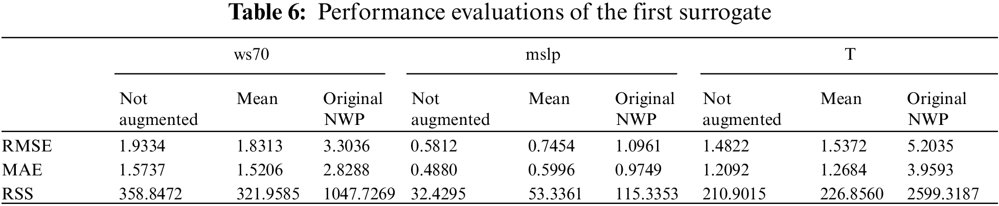
The first surrogate contains three sub-surrogates that are trained with D^trainws70, D^trainmslp, and D^trainT, respectively. The original sample without augmentation is used to verify the ELMs training effect and generalization ability during training to avoid overfitting. The training is considered complete when the network, which is trained with augmented data, can properly generalize the original sample. After training, the forecasting dataset D^forecastws70/mslp/T is input to produce calibrated forecasting results for SFs (ws70, mslp, and T). As shown in Fig. 10, the blue lines denote the real monitored weather factors, and the 95% confidence intervals (CI) of the calibrated forecasting results are shown with the shadow area between red lines, and the green line denotes the mean of calibration. The original NWP data are shown in purple lines, and the forecasting results with the not augmented dataset Dforecastws70/mslp/T are shown in yellow lines. Commonly used performance evaluation indicators for accuracy, i.e., RMSE, MAE, and RSS, are listed in Table 5, together with three commonly used probabilistic performance evaluation indicators PICP, ACE, and PINAW. The smaller the value of RMSE, MAE, RSS, ACE, and PINAW, the better the result. Conversely, larger values of PICP indicate better results. Table 6 lists the accuracy evaluation results for the first surrogate. As shown in Fig. 10 and Table 6 after calibrating, the prediction accuracies of these three SFs are all improved, especially for the ws70 and T. As shown in Fig. 10, there is a certain difference between the mean of the prediction results using the augmented forecasting data and the prediction results using the raw forecasting data. This is because the augmentation using WWGAN is not just calculating raw data's quantile but learning the time-varying distribution patterns of it, that is, its physical information. As seen from the Fig. 10 and Table 6, the raw NWP data is calibrated through the first surrogate with a smaller error between the real value.

Figure 10: Calibrated SFs (ws70, mslp, T) and the 95% CI

4.3.2 The Second AI Surrogate

The second AI surrogate is trained with DtrainWP, the historical SFs, and wind power. Due to the high relevance between SFs and wind power, the ELM network's generalization ability can be trained on and verified on the same training datasets. The training effects of the second surrogate are shown in Fig. 11. The ELM model's validation effect on the training set is adequate, and the predicted wind power generation is close to the actual power generation, as shown in Fig. 11.

Figure 11: The training effects of the second surrogate

When training is completed, the outputs from the first surrogate were used as inputs to produce the probabilistic forecasting result for wind power. After denormalization, the forecasting results from 2016-3-4 00:00:00 to 2016-3-4 23:45:00 are shown in Fig. 12 with a resolution of 15 min. Here the blue line represents the real wind power data, the green line denotes the forecast result, and the yellow line represents the mean estimate of the forecast result. Both the accuracy and probabilistic performance evaluation results are shown in Table 7. In Table 7, RMSE, MAE, and SSE are calculated using the not augmented prediction results, while PICP, ACE, and PINAW are calculated using the set of augmented prediction results.

Figure 12: Probabilistic forecasting result from the second surrogate

4.4 Discussion

In order to evaluate the forecasting effect of the proposed method, three mainstream wind power forecasting methods are selected as benchmarks, the ELM-based method [34], the method based on the combination of VMD and LSTM (VMD-LSTM) [32], the Bayesian model (BM) [27] and the CNN-LSTM [30]. Among them, the VMD-LSTM class method first uses VMD to decompose training input data and labels into ten modes and then uses LSTM to perform regression learning mode by mode. After learning, the prediction data is also decomposed into ten modes and poured into the corresponding LSTM to obtain the output respectively, then add up the output results of all modes for the final result. Through VMD, the uncertainty is also decomposed, thus diminishing the difficulty of uncertainty quantification and improving the learning efficiency of LSTM. At the same time, to further verify the impact of the training and testing datasets on the prediction effect, the not augmented real weather factors and NWP data were used as training or testing sets to compare with the proposed data augmentation approach. Specifically, 12 wind power probabilistic forecasting approaches are compared with the proposed AI surrogates method, as shown in Table 8. The prediction accuracy and probabilistic performance are mainly discussed here, so denormalization is not performed. The evaluation results are shown in Table 8 and Fig. 13.

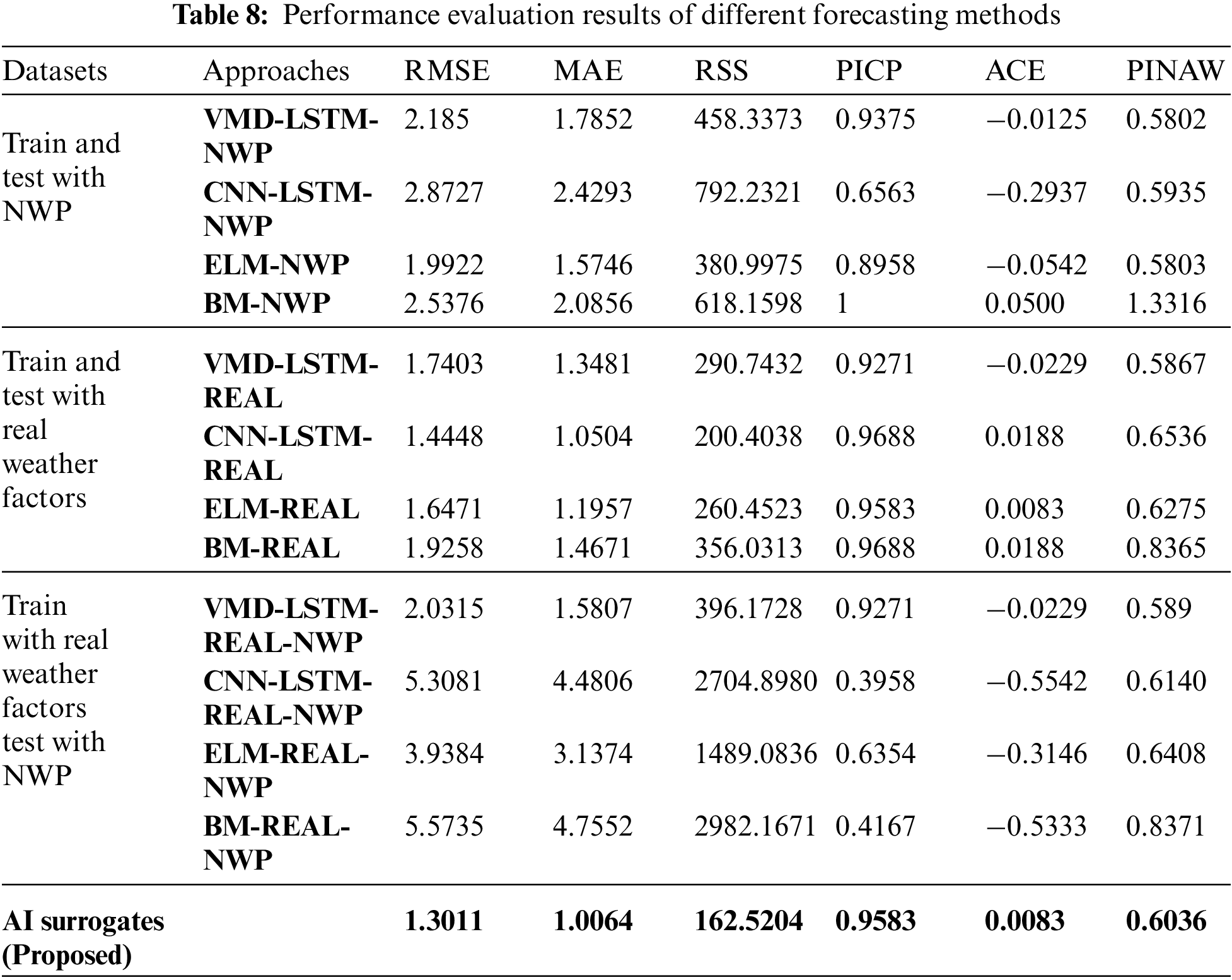
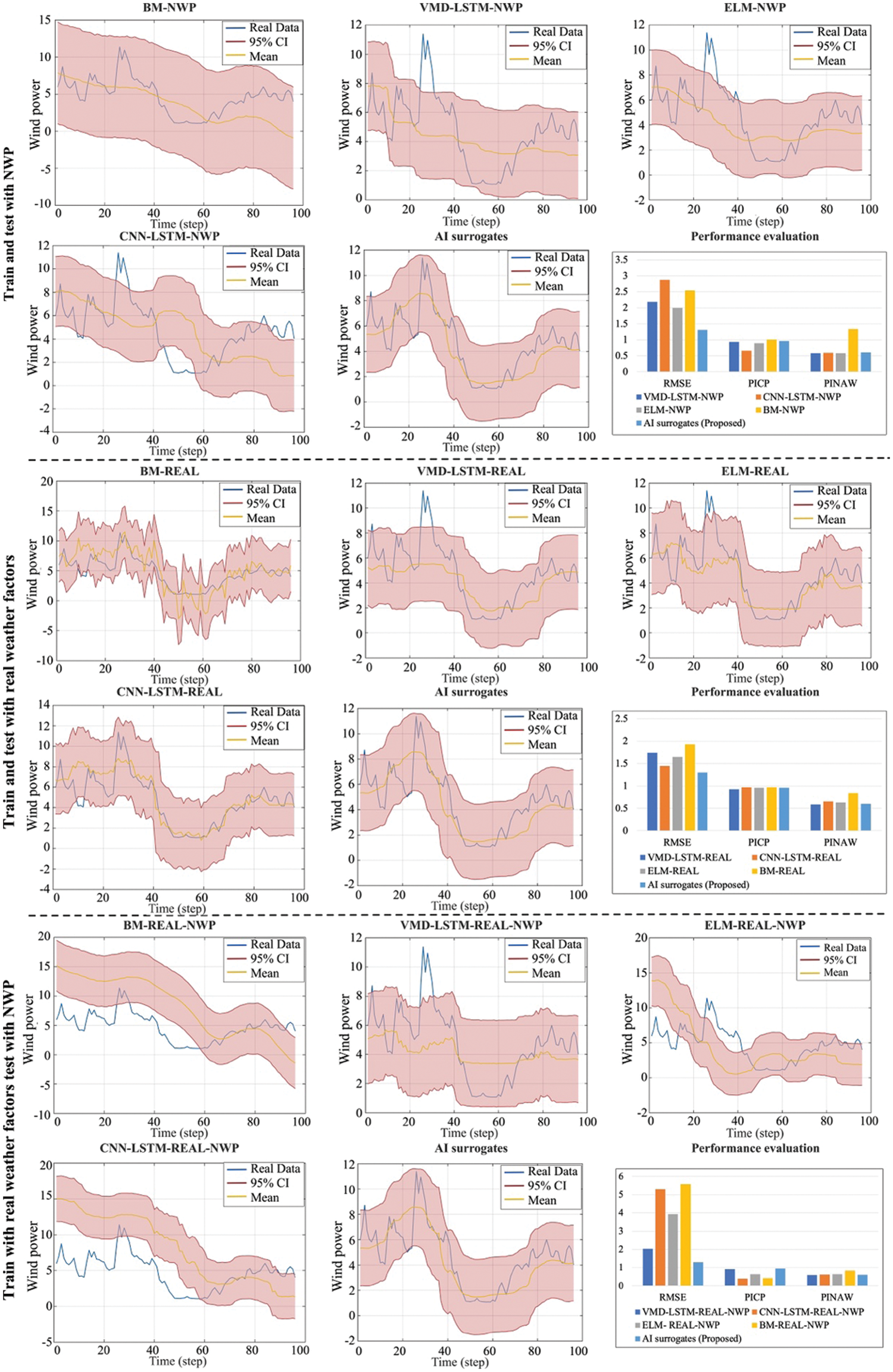
Figure 13: Evaluation results of different methods with different datasets

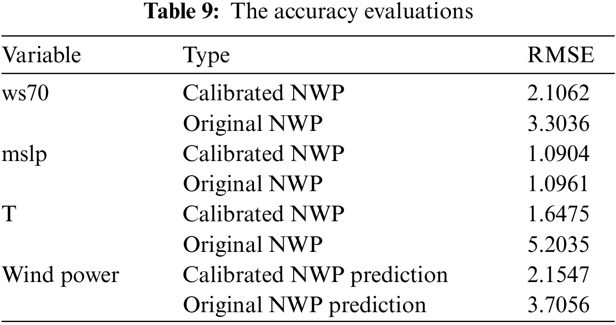
In Fig. 13, approaches that use the same training and testing sets are grouped and compared with the proposed method to verify the performance with a bar chart of evaluation attached. In each group, the probabilistic forecasting results of benchmark and proposed methods are exhibited by line charts. Within each line chart, the mean values of prediction results are shown in yellow lines, the real power generation is shown in blue, and the red area shows the 95% CI of prediction results. The bar chart in each group exhibits the RMSE, PICP, and PINAW of the prediction results from each approach. The results in Table 9 and Fig. 13 show that the proposed method can provide the best prediction accuracy and the most realistic probability performance compared with the benchmarks. Different training and testing sets do affect the performance of forecasting, and training and testing with real weather factors can achieve the best accuracy. However, the real weather factors cannot be obtained a day ahead, which makes models trained with it more appropriate for real-time modeling tasks but cannot handle day-ahead forecasting. In contrast, the uncertainty in NWP data limits the prediction accuracy of models trained on it. As for training with real weather data and then testing with NWP data, neither the accuracy nor the probabilistic performance is adequate due to the mismatch between the training and testing datasets.

Note that the proposed method exceeds the approaches trained and tested with real weather factors, as shown in Fig. 13. This is because the real weather factors and power generation dataset, which, as mentioned, is an incomplete training set. Hence, the incomplete mapping between weather features and wind power generation in the dataset constraints the generalization ability of models trained on it. While after using the proposed method to augment the training data, some missing or fewer features are supplemented, thereby improving the generalization ability of the prediction model. The results indicate that, through data augmentation and multiple AI surrogates, the proposed method obtained the intrinsic physics information from NWP data and quantified its uncertainty, effectively calibrating the day-ahead weather forecasting outputs. Compared with other wind power probabilistic forecasting methods, the proposed method has a better training effect on an incomplete dataset. The prediction accuracy, generalization ability, and probability prediction effect are more reliable.

In order to further verify the effect of the proposed method on a smaller data set, the training set is reduced to half. Only the data from 2016-2-26 to 2016-3-3 are used as training data. Employ the proposed method to build surrogates and predict the wind power generation in 2016-3-4. The training and testing process remains unchanged; the results are shown in Fig. 14. As shown in Fig. 14, the original NWP of ws70, mslp, and T are calibrated with the first surrogate, and with the calibrated NWP data, the prediction result of wind power generation is obtained. Table 9 shows the RMSE evaluations. Although only one week of training data is employed, the proposed method can still improve the effect of wind power forecasting. However, there is an accuracy gap compared to the forecast results using two weeks of data which means a certain amount of data is necessary for accurate forecasting.

Figure 14: Forecasting results with one-week training data

5  Conclusion

This article aims at the operation and management of renewable energy smart grids for smart cities and buildings. A physics-informed AI surrogates method for probabilistic forecasting of wind power generation is introduced to tackle the insufficient generalization ability of high-resolution day-ahead forecasting caused by incomplete datasets. The proposed method is able to mine the implicit physical information in NWP data by employing small sample augmentation algorithms based on GAN, then train the forecasting model with a multiple AI surrogates structure constructed with ELM. Thus, the uncertainty within the NWP data and wind power generation are modeled and quantified. Compared with conventional probabilistic forecasting methods, the proposed method improves in these three aspects:

1.    Compared with conventional methods, the proposed method improves the accuracy and probability forecasting performance of day-ahead wind power generation forecasting, tested on a certain incomplete dataset of a particular wind power farm.

2.    Through incomplete data augmentation, the proposed method enhances the training effect and generalization ability of the prediction model on the one hand and, on the other hand, provides a more extensive data basis for quantifying the uncertainty of the prediction results. This characteristic makes it applicable for relatively small datasets with missing, discontinuous, and abnormal data. Therefore, considering the fluctuating nature of renewable energy, the proposed method’s prospects in modeling and controlling renewable energy smart grids are apparent.

3.    The prediction model constructed by multiple AI surrogates enables the wind power prediction model trained on real weather factors to provide accurate wind power prediction with NWP data. Therefore, it is possible to calibrate the prediction model in real-time through the weather and wind power data monitored online to ensure its prediction ability, which is meaningful for the power generation simulation tasks in the digital twin of smart cities.

Funding Statement: This work was funded by the National Natural Science Foundation of China under Grant 62273022.

Conflicts of Interest: The authors declare that they have no conflicts of interest to report regarding the present study.

References

1. Fan, D., Ren, Y., Feng, Q., Liu, Y., Wang, Z. et al. (2021). Restoration of smart grids: Current status, challenges, and opportunities. Renewable and Sustainable Energy Reviews, 143, 110909. https://doi.org/10.1016/j.rser.2021.110909 [Google Scholar] [CrossRef]

2. Judge, M. A., Khan, A., Manzoor, A., Khattak, H. A. (2022). Overview of smart grid implementation: Frameworks, impact, performance and challenges. Journal of Energy Storage, 49, 104056. https://doi.org/10.1016/j.est.2022.104056 [Google Scholar] [CrossRef]

3. Giebel, G., Draxl, C., Shaw, W., Zack, J., Kariniotakis, G. et al. (2020). IEA wind task 36–An overview. Presented at the 19th Wind Integration Workshop, pp. 1–3. Virtual Event, Germany. [Google Scholar]

4. Ahmad, T., Zhang, H., Yan, B. (2020). A review on renewable energy and electricity requirement forecasting models for smart grid and buildings. Sustainable Cities and Society, 55, 102052. https://doi.org/10.1016/j.scs.2020.102052 [Google Scholar] [CrossRef]

5. Ali, S., Ullah, K., Hafeez, G., Khan, I., Albogamy, F. R. et al. (2022). Solving day-ahead scheduling problem with multi-objective energy optimization for demand side management in smart grid. Engineering Science and Technology, an International Journal, 36, 101135. https://doi.org/10.1016/j.jestch.2022.101135 [Google Scholar] [CrossRef]

6. Ren, Y., Fan, D., Feng, Q., Wang, Z., Sun, B. et al. (2019). Agent-based restoration approach for reliability with load balancing on smart grids. Applied Energy, 249, 46–57. https://doi.org/10.1016/j.apenergy.2019.04.119 [Google Scholar] [CrossRef]

7. Scarabaggio, P., Grammatico, S., Carli, R., Dotoli, M. (2022). Distributed demand side management with stochastic wind power forecasting. IEEE Transactions on Control Systems Technology, 30(1), 97–112. https://doi.org/10.1109/TCST.2021.3056751 [Google Scholar] [CrossRef]

8. Wang, Y., Zou, R., Liu, F., Zhang, L., Liu, Q. (2021). A review of wind speed and wind power forecasting with deep neural networks. Applied Energy, 304, 117766. https://doi.org/10.1016/j.apenergy.2021.117766 [Google Scholar] [CrossRef]

9. Yousuf, M. U., Al-Bahadly, I., Avci, E. (2022). Wind speed prediction for small sample dataset using hybrid first-order accumulated generating operation-based double exponential smoothing model. Energy Science & Engineering, 10(3), 726–739. https://doi.org/10.1002/ese3.1047 [Google Scholar] [CrossRef]

10. Fan, D., Ren, Y., Feng, Q., Zhu, B., Liu, Y. et al. (2019). A hybrid heuristic optimization of maintenance routing and scheduling for offshore wind farms. Journal of Loss Prevention in the Process Industries, 62, 103949. https://doi.org/10.1016/j.jlp.2019.103949 [Google Scholar] [CrossRef]

11. Fan, H., Wang, C., Liu, L., Li, X. (2022). Review of uncertainty modeling for optimal operation of integrated energy system. Frontiers in Energy Research, 9, 641337. https://doi.org/10.3389/fenrg.2021.641337 [Google Scholar] [CrossRef]

12. Khajeh, H., Laaksonen, H. (2022). Applications of probabilistic forecasting in smart grids: A review. Applied Sciences, 12(4), 1823. https://doi.org/10.3390/app12041823 [Google Scholar] [CrossRef]

13. Raissi, M., Perdikaris, P., Karniadakis, G. E. (2019). Physics-informed neural networks: A deep learning framework for solving forward and inverse problems involving nonlinear partial differential equations. Journal of Computational Physics, 378, 686–707. https://doi.org/10.1016/j.jcp.2018.10.045 [Google Scholar] [CrossRef]

14. Karniadakis, G. E., Kevrekidis, I. G., Lu, L., Perdikaris, P., Wang, S. et al. (2021). Physics-informed machine learning. Nature Reviews Physics, 3(6), 422–440. https://doi.org/10.1038/s42254-021-00314-5 [Google Scholar] [CrossRef]

15. Shao, H., Lin, J., Zhang, L., Galar, D., Kumar, U. (2021). A novel approach of multisensory fusion to collaborative fault diagnosis in maintenance. Information Fusion, 74, 65–76. https://doi.org/10.1016/j.inffus.2021.03.008 [Google Scholar] [CrossRef]

16. Sun, B., Wu, Z., Feng, Q., Wang, Z., Ren, Y. et al. (2022). Small sample reliability assessment with online time-series data based on a worm WGAN learning method. IEEE Transactions on Industrial Informatics, 19(2), 1207–1216. https://doi.org/10.1109/TII.2022.3168667 [Google Scholar] [CrossRef]

17. Che, Y., Salazar, A. A., Peng, S., Zheng, J., Chen, Y. et al. (2022). A multi-scale model for day-ahead wind speed forecasting: A case study of the Houhoku wind farm, Japan. Sustainable Energy Technologies and Assessments, 52(A), 101995. https://doi.org/10.1016/j.seta.2022.101995 [Google Scholar] [CrossRef]

18. Cuevas-Figueroa, G., Stansby, P. K., Stallard, T. (2022). Accuracy of WRF for prediction of operational wind farm data and assessment of influence of upwind farms on power production. Energy, 254, 124362. https://doi.org/10.1016/j.energy.2022.124362 [Google Scholar] [CrossRef]

19. Zhang, G., Zheng, X., Liu, S., Chen, M., Wang, C. et al. (2022). Three-dimensional wind velocity reconstruction based on tensor decomposition and CFD data with experimental verification. Energy Conversion and Management, 256, 115322. https://doi.org/10.1016/j.enconman.2022.115322 [Google Scholar] [CrossRef]

20. Deng, X., Shao, H., Hu, C., Jiang, D., Jiang, Y. (2022). Wind power forecasting methods based on deep learning: A survey. Computer Modeling in Engineering & Sciences, 122(1), 273–301. https://doi.org/10.32604/cmes.2020.08768 [Google Scholar] [CrossRef]

21. Ji, T., Wang, J., Li, M., Wu, Q. (2022). Short-term wind power forecast based on chaotic analysis and multivariate phase space reconstruction. Energy Conversion and Management, 254, 115196. https://doi.org/10.1016/j.enconman.2021.115196 [Google Scholar] [CrossRef]

22. Sun, W., Wang, Y. (2018). Short-term wind speed forecasting based on fast ensemble empirical mode decomposition, phase space reconstruction, sample entropy and improved back-propagation neural network. Energy Conversion and Management, 157, 1–12. https://doi.org/10.1016/j.enconman.2017.11.067 [Google Scholar] [CrossRef]

23. Liu, Y., Qin, H., Zhang, Z., Pei, S., Jiang, Z. et al. (2020). Probabilistic spatiotemporal wind speed forecasting based on a variational Bayesian deep learning model. Applied Energy, 260, 114259. https://doi.org/10.1016/j.apenergy.2019.114259 [Google Scholar] [CrossRef]

24. Zhou, B., Duan, H., Wu, Q., Wang, H., Or, S. W. et al. (2021). Short-term prediction of wind power and its ramp events based on semi-supervised generative adversarial network. International Journal of Electrical Power & Energy Systems, 125, 106411. https://doi.org/10.1016/j.ijepes.2020.106411 [Google Scholar] [CrossRef]

25. Wan, C., Lin, J., Wang, J., Song, Y., Dong, Z. Y. (2017). Direct quantile regression for nonparametric probabilistic forecasting of wind power generation. IEEE Transactions on Power Systems, 32(4), 2767–2778. https://doi.org/10.1109/TPWRS.2016.2625101 [Google Scholar] [CrossRef]

26. Mehdi, N., Meysam, M. N., Ehsan, A., Seyedali, M., Daniele, G. et al. (2021). Wind turbine power output prediction using a new hybrid neuro-evolutionary method. Energy, 229, 120617. https://doi.org/10.1016/j.energy.2021.120617 [Google Scholar] [CrossRef]

27. Victor, E. D., Thais, C. F., Fernando, L. C. O. (2022). Joint modelling wind speed and power via Bayesian dynamical models. Energy, 247, 123431. https://doi.org/10.1016/j.energy.2022.123431 [Google Scholar] [CrossRef]

28. Boudy, B., Kondo, H. A., Alexandre, S., Kaan, Y., Emel, K. (2022). Wind power conversion system model identification using adaptiveneuro-fuzzy inference systems: A case study. Energy, 239, 122089. https://doi.org/10.1016/j.energy.2021.122089 [Google Scholar] [CrossRef]

29. Wu, Y. K., Wu, Y. C., Hong, J. C. S., Phan, L. H., Phan, Q. D. (2021). Probabilistic forecast of wind power generation with data processing and numerical weather predictions. IEEE Transactions on Industry Applications, 57(1), 36–45. https://doi.org/10.1109/TIA.28 [Google Scholar] [CrossRef]

30. He, B., Ye, L., Pei, M., Lu, P., Dai, B. et al. (2022). A combined model for short-term wind power forecasting based on the analysis of numerical weather prediction data. Energy Reports, 8, 929–939. https://doi.org/10.1016/j.egyr.2021.10.102 [Google Scholar] [CrossRef]

31. Xia, B., Huang, Q., Wang, H., Ying, L. (2022). Wind power prediction in view of ramping events based on classified spatiotemporal network. Frontiers in Energy Research, 9, 754274. https://doi.org/10.3389/fenrg.2021.754274 [Google Scholar] [CrossRef]

32. Han, Y., Mi, L., Shen, L., Cai, S., Liu, Y. et al. (2022). A short-term wind speed interval prediction method based on WRF simulation and multivariate line regression for deep learning algorithms. Energy Conversion and Management, 258, 115540. https://doi.org/10.1016/j.enconman.2022.115540 [Google Scholar] [CrossRef]

33. Huang, G. B., Zhu, Q. Y., Siew, C. K. (2004). Extreme learning machine: A new learning scheme of feedforward neural networks. 2004 IEEE International Joint Conference on Neural Networks, vol. 2, pp. 985–990. [Google Scholar]

34. Wan, C., Xu, Z., Pinson, P., Dong, Z. Y., Wong, K. P. (2014). Probabilistic forecasting of wind power generation using extreme learning machine. IEEE Transactions on Power Systems, 29(3), 1033–1044. https://doi.org/10.1109/TPWRS.2013.2287871 [Google Scholar] [CrossRef]

35. Goodfellow, I. J., Pouget-Abadie, J., Mirza, M., Xu, B., Warde-Farley et al. (2014). Generative adversarial networks. 28th Conference on Neural Information Processing Systems (NIPS), pp. 2672–2680. Montreal, Canada. [Google Scholar]

36. Li, W., Zhong, X., Shao, H., Cai, B., Yang, X. (2022). Multi-mode data augmentation and fault diagnosis of rotating machinery using modified ACGAN designed with new framework. Advanced Engineering Informatics, 52, 101552. https://doi.org/10.1016/j.aei.2022.101552 [Google Scholar] [CrossRef]

37. Yun, W., Lu, Z., Jiang, X. (2018). An efficient reliability analysis method combining adaptive kriging and modified importance sampling for small failure probability. Structural and Multidisciplinary Optimization, 58(4), 1383–1393. https://doi.org/10.1007/s00158-018-1975-6 [Google Scholar] [CrossRef]

38. Amalnerkar, E., Lee, T. H., Lim, W. (2020). Reliability analysis using bootstrap information criterion for small sample size response functions. Structural and Multidisciplinary Optimization, 62(6), 2901–2913. https://doi.org/10.1007/s00158-020-02724-y [Google Scholar] [CrossRef]

39. He, Z., Shao, H., Lin, J., Cheng, J., Yang, Y. (2020). Transfer fault diagnosis of bearing installed in different machines using enhanced deep auto-encoder. Measurement, 152, 107393. https://doi.org/10.1016/j.measurement.2019.107393 [Google Scholar] [CrossRef]

40. Arjovsky, M., Chintala, S., Bottou, L. (2017). Wasserstein generative adversarial networks. International Conference on Machine Learning, pp. 214–223. Sydney, Australia. [Google Scholar]

41. Gulrajani, I., Ahmed, A., Arjovsky, M., Dumoulin, V., Courville, A. C. (2017). Improved training of wasserstein gans. Advances in Neural Information Processing Systems, 30, 1–20. [Google Scholar]

42. Li, X., Cheng, J., Shao, H., Liu, K., Cai, B. (2022). A fusion CWSMM-based framework for rotating machinery fault diagnosis under strong interference and imbalanced case. IEEE Transactions on Industrial Informatics, 18(8), 5180–5189. https://doi.org/10.1109/TII.2021.3125385 [Google Scholar] [CrossRef]

43. Peng, H., Long, F., Ding, C. (2005). Feature selection based on mutual information criteria of max-dependency, max-relevance, and min-redundancy. IEEE Transactions on Pattern Analysis and Machine Intelligence, 27(8), 1226–1238. https://doi.org/10.1109/TPAMI.2005.159 [Google Scholar] [PubMed] [CrossRef]

44. Li, X., Shao, H., Lu, S., Xiang, J., Cai, B. (2022). Highly-efficient fault diagnosis of rotating machinery under time-varying speeds using LSISMM and small infrared thermal images. IEEE Transactions on Systems, Man, and Cybernetics: Systems, 52(12), 7328–7340. https://doi.org/10.1109/TSMC.2022.3151185 [Google Scholar] [CrossRef]

Supplementary Materials

Supplementary Figure S1: The data augmentation result for Dtrainmslp

Supplementary Figure S2: The data augmentation result for DtrainT