An Improved Soft Subspace Clustering Algorithm for Brain MR Image Segmentation

1  Introduction

A clustering algorithm is an unsupervised way of dividing a set of data objects into different clusters so that the similarity between clusters is enhanced and reduced. In recent years, the development of artificial intelligence algorithms has led to the use of clustering as a powerful data analysis tool, which is often used in a number of fields. Examples include artificial intelligence [1], image segmentation [2], community detection [3], image classification, etc. In recent years, medical imaging has made considerable breakthroughs in clustering algorithms, which can be used to segment images. The clustering algorithms also play a very important role in the examination of medical images. The existing magnetic resonance imaging (MRI) has the advantage of good soft tissue resolution, high spatial resolution and arbitrary three-dimensional imaging, which allows for clearer segmentation of organs, accurate identification of lesions and differentiation of various parts of the soft tissue, which is easy for doctors to view. In recent years, MRI has gradually been adopted as the primary examination modality for lesion detection in China and abroad [4,5]. However, in the imaging process, there are always multiple random noises in the image due to external uncertainties and a series of problems, such as uneven grayscale and blurred boundaries, which make segmentation difficult. The clustering algorithm itself is also degraded by the problem of being easily trapped in a local optimum [6]. This paper presents a large breakthrough in MR image segmentation by introducing generalized noise detection techniques and enhancing the noise immunity of the algorithm.

The fuzzy C-means clustering algorithm (FCM) classifies images into one or more classes according to specific information features. The traditional soft subspace clustering algorithm is based on the fuzzy weighted approach of the FCM, which divides the total number of data into different cluster classes. The FCM-based algorithm provides high segmentation accuracy for MR image segmentation [7,8]. However, due to the numerous idiosyncrasies of the features in the image, many feature attributes are only associated with a portion of the subspace, often resulting in missing and invalid spatial information. Two major drawbacks in the FCM-based algorithm are as follows: (1) it can cause noise anomalies and noise sensitivity, and (2) it is an iterative descent algorithm, which is not conducive to finding the global optimum. Therefore, in later studies, Agrawal et al. first introduced subspace clustering (SC) [9], which then evolved into a contest between hard subspace clustering (HSC) and soft subspace clustering (SSC) [10]. Typical algorithms include entropy weighting K-means (EWKM), local adaptive clustering (LAC), fuzzy subspace clustering (FSC) [11] and weighted Minkowski metric weighted K-Means (MWK-Means) [12]. Later, some optimization algorithms were proposed for the algorithmic problem, including quantum behavior particle swarm optimization (SSC-QPSO) [13], artificial colony soft subspace clustering (ACSSC) [14], and a soft subspace clustering algorithm based on random walk (RWSSC) [15]. There are also soft subspace clustering algorithms for use for high-dimensional data: entropy-weighting streaming subspace clustering (EWSSC) [16]. These algorithms are highly scalable and relatively flexible in application but are susceptible to dependence on initial clustering centers and fall into local optima, as well as sensitivity to noise, when clustering brain MR images. In 2019, Fan et al. proposed optimizing the soft subspace clustering algorithm for breast MR images using a brainstorming algorithm (BSASSC) [17]. The local and global search performance was well balanced, and the clustering effect was good for brain MR images, but there were still boundary inaccuracies in the BSASSC algorithm for MR image segmentation. In contrast to other population intelligence optimization algorithms, such as particle swarm algorithms [18], artificial fish swarm algorithms [19], and flower pollination algorithms [20], genetic algorithms [21] are a class of parallel stochastic search optimization methods constructed artificially to simulate natural biogenetics and biological evolution and to illustrate the principle of “survival of the fittest”. Thus, this paper describes combining a genetic algorithm with a soft subspace clustering method to better balance the global and local correspondence and enhance the intraclass tightness and interclass separation to optimize the cluster center. Combined with the generalized noise technique [22], we propose a soft subspace clustering algorithm for brain MR images based on genetic algorithm optimization to compensate for the deficiency that the existing soft subspace clustering algorithm easily falls into the local optimum and improve the accuracy of the algorithm, which will have a positive effect on clinical medicine [23].

In this paper, based on the fuzzy C mean clustering algorithm, for the algorithm of clustering the center into the local optima and the clustering strategy for the optimization algorithm, we attempt to combine the intelligent group optimization algorithm. Relying on the literature, the final genetic algorithm chosen for the initial clustering center, compared with other clustering algorithms, focuses on the initial clustering center. The algorithm proposed in this paper is used in brain MR image segmentation. Because the brain MR images contain high noise, boundary blur and other problems, the algorithm is able to solve the noise problem. This paper adds generalized noise processing technology into the fuzzy C mean clustering algorithm, which is committed to solving the existing problems of medical images.

2  Introduction of Related Algorithms

2.1 Soft Subspace Clustering Algorithms

Given a data matrix X with N samples in a D-dimensional space, the purpose of soft subspace clustering is to classify these datasets X into different clusters and obtain the clustering centers corresponding to the C cluster V=(V1,V2,…,VC) and feature weights W=(W1,W2,…,WC). Wi=(i=1,2,…,C) denotes the feature weights of the ith cluster. The development of soft subspace clustering has been long overdue. Due to the better adaptability and flexibility of soft subspace algorithms [24], they have gained wide attention and some development has been made. The soft subspace algorithm considers that each attribute of the original data is meaningful to the cluster and measures the degree of contribution of each dimensional feature to a specific cluster according to the weight value of the attribute; the larger the weight value is, the more important it is. Soft subspace clustering can be seen as an extension of the traditional feature-weighted clustering algorithm, and depending on the way the attributes are weighted, it can be divided into fuzzy weighting [25] and entropy weighting algorithms [26]. The fuzzy weighted soft subspace clustering algorithm is used to describe the uncertainty of samples belonging to different clusters by fuzzy weights, i.e., the importance of features for clusters. The most important factors affecting the clustering model of the soft subspace depend on different weighting methods and on the initialization selection of the cluster center. In previous studies, many different selection strategies were proposed.

An attribute weighting algorithm (AWA) with attribute weighting was proposed by Chan et al. [27] in 2004. This is the earliest fuzzy weighted soft subspace clustering algorithm. The AWA algorithm can effectively discover the important features of each cluster by introducing fuzzy affiliation and a fuzzy weight index to assign a different weight to each dimensional feature of each data cluster. However, the AWA algorithm loses its meaning when the standard deviation of some attributes is zero. The objective function of the AWA algorithm is shown in Eq. (1) as follows:

JAWA=∑i=1C∑j=1NUij∑k=1DWikτ(Xjk−Vik)2s.t. Uij∈{0,1}, ∑i=1CUij=1,0<∑j=1NUij<1, and ∑k=1DWik=1(1)

The AWA algorithm overcomes this drawback and prevents one of the dimensions from obtaining all the weights while some of the dimensions are missing weights. Gan et al. proposed a fuzzy subspace clustering (FSC) [28] algorithm in 2008 by introducing a weight penalty term in the objective function. The objective function of the FSC algorithm is shown in Eq. (2) as follows:

JFSC=∑i=1C∑j=1NUij∑k=1DWikτ(Xjk−Vik)2+ε∑i=1C∑K=1DWikτs.t. Uij∈{0,1}, ∑i=1CUij=1,0<∑j=1NUij<1, and ∑k=1DWik=1(2)

The first term of the objective function represents the weighted distance of all data points to their respective cluster centers; the smaller the first term is, the more compact its clusters are. The second term on the right side of the medium sign of the objective function is a weight constraint.

The role of the second term is to minimize the tightness between clusters [29] and to balance the weights over the different dimensions. If the weights are not completely released, it will have a detrimental effect; one of the dimensions obtains all the weights, while the rest of the dimensions do not have any weight values, which will cause uneven results and poor clustering. However, the FSC algorithm only improves the objective function for intraclass coupling but ignores the dispersion between classes. The FSC algorithm also exists: (1) sensitivity to initial values, and (2) when the data dimension is too large [30], the corresponding subspace cannot be utilized well, resulting in dimensional disasters. The convergence of the FSC in the face of high-dimensional data was discussed by Gan et al. in 2008 [31], and the objective function was improved by fuzzy weighting; it has good adaptability to different datasets after setting fuzzy coefficients compared with the classical weighting approach, but once out of the influence of noise, the fuzzy weighting approach does not perform robustly. When targeting high-dimensional data [31,32], the FSC algorithm estimates feature weight values for each cluster, improving the objective function only for intraclass coupling but ignoring interclass dispersion [33].

Another classical strategy to control the weight distribution in the soft subspace clustering algorithm is to use the maximum entropy weighting strategy, assuming that the introduction of a good weight for each latitude is different; when a weight is given, although some dimension weights are small, it is also necessary to have. Therefore, entropy weighting plays a smoothing role so that the weighting of each item will be smoother, and thus, the whole generation value will decrease. Representative soft subspace clustering algorithms with the entropy weighting approach include EWKM [34] and LAC [35]. The entropy-weighted soft subspace clustering algorithm differs from the fuzzy weighting approach in that it effectively controls the weight distribution through the entropy term. In 2007, Jing et al. introduced the maximum information entropy theory into a soft subspace algorithm and proposed an entropy weighted K-Means algorithm (EWKM), which uses weight entropy and weighted in-class similarity as penalty terms to optimize targets [36]. The weighted index can effectively avoid the situation in which the weight of a certain cluster class is 0. The algorithm expression of EWKM is shown in Eq. (3) as follows:

JEWKM=∑i=1C∑j=1NUij∑k=1DWik(Xjk−Vik)2+λ∑i=1C∑k=1DWikln⁡(Wik)s.t. Uij∈{0,1}, ∑i=1CUij=1,0<∑j=1NUij<1, and ∑k=1DWik=1(3)

The second term in the objective function is a negative Shannon entropy, and λ is used to balance its influence on the clustering process. EWKM can effectively control the weight distribution by introducing the entropy term and has become a basic independent soft subspace clustering algorithm (ISSC) [37]. Deng et al. [38] proposed an enhanced soft subspace clustering (ESSC) algorithm by introducing the weighted interclass separation and spatial information into the objective function for the first time on the basis of EWKM.

The information of interclass separateness is introduced while maximizing intraclass tightness to effectively enhance the effect of subspace clustering, and the objective function is shown in Eq. (4) as follows:

JESSC=∑i=1C∑j=1NUijm∑k=1DWik(Xjk−Vik)2+λ∑i=1C∑k=1DWikln⁡(Wik)−η∑i=1C∑j=1NUijm∑k=1DWik(Vik−Vok)2s.t. Uij∈{0,1}, ∑i=1CUij=1,0<∑j=1NUij<1,0≤Wik≤1, and ∑k=1DWik=1(4)

where λ is the control entropy weighting, η controls the separation between classes, and the index of affiliation m controls the fuzzy index. The ESSC algorithm proposes enhanced soft subspace clustering based on intraclass and interclass features. The aim of this algorithm is intended to effectively reduce the impact of the cluster class center and the global center of similar features to cause clustering between whole clusters. Then, we need to pay attention to these points for improvement: (1) We calculate the distance between the sample points belonging to different clusters. (2) We calculate the distance between the cluster center and the global center well. However, there are still problems in the iterative process of the algorithm, such as that the optimal clustering effect cannot be obtained because the structural formula cannot be differentiated [39], and the parameters are not introduced reasonably, so the algorithm is not generalized enough.

The algorithm that fuses intraclass compactness and interclass separateness can achieve better clustering results [40]. Therefore, the subspace clustering algorithm should fuse more discriminative information, such as intraclass and interclass information, when constructing the objective function to improve the algorithm’s performance. The innovation of the ESSC algorithm lies in the following: (1) The division of enhanced intracluster compactness and intercluster separateness is adopted simultaneously. (2) The robustness of the algorithm and its tolerance to the parameters are reflected. The synthesized dataset becomes increasingly realistic in terms of meaning.

In the subsequent algorithms, the algorithm relaxes the complex equation constraints in the search process to bound constraints and reduces the weight complexity in the objective function in the process of finding the best. These improved algorithms make a greater contribution to soft subspace clustering.

2.2 Noise Clustering Algorithm Research

Most image clustering algorithms use image feature information to segment the image, such as grayscale information and textural information, but ignore the impact of noisy data on the clustering algorithm. The clustering algorithm is sensitive to the noise problem and is the focus of our research. To address the data sensitivity problem of noisy data in the clustering process, Davé et al. proposed the generalized noise clustering (GNC) algorithm [41], whose objective function is shown in Eq. (5) as follows:

JGNC(U,V)=∑i=1C∑k=1NUijmDik2+∑i=1C∑k=1Nδik2(1−∑i=1CUik)m(5)

where Dik=||Xk−Vi|| represents the Euclidean distance from each data point to the center of the cluster δik2=ηi∗Uik∗ is the middle parameter from the possibilistic C-means clustering (PCM) [42], and its formula is shown in Eq. (6). The Uik∗ with the same formula for calculating the affiliation of the FCM formulated in Eq. (7) as follows:

ηi=β⋅∑k=1NUikm,FCM⋅Dik2∑k=1NUikm,FCM,β>0(6)

Uik∗=[∑j=1C(DikDjk)2m−1]−1,∀i,k(7)

The calculation formula of the GNC algorithm cluster center is shown in Eq. (8) as follows:

Vi=∑k=1NUikm⋅Xk∑k=1NUikm,∀i(8)

The noise clustering algorithm can effectively solve some noise problems in medical images and can present new breakthroughs in MR image processing.

2.3 Study of the Genetic Algorithm

The genetic algorithm [43] was first proposed by Bagley, a student of Professor J. Holland at the University of Michigan in 1967, who discussed one of the intelligent population optimization algorithms, the genetic algorithm, in his doctoral dissertation. In his PhD thesis, he discussed one of the intelligent population optimization algorithms, the genetic algorithm, but due to the lack of knowledge and the lack of computational tools, the theory was only at the primary stage until 1975, when J. Holland et al. conceived the key theoretical model for the genetic algorithm; the genetic algorithm is an optimization method that simulates natural biogenetics (Mendel) and biological evolution (Darwin) by constructing a parallel random search in an artificial way. This theory illustrates the natural law of survival: “survival of the fittest”.

Genetic algorithms are composed of chromosome encoding, finding fitness functions, genetic operations and parameter runs. There are three types of chromosome encoding: binary encoding, symbolic encoding and real encoding. From these three encoding methods, the coding problem is chosen to form a set of chromosomes, with each set of chromosomes acting as individuals. An initial population is formed from multiple individuals, and parameters, such as the number of chromosomes in this population, the probability of variation and the number of iterations, are determined. Then, the population iteration is terminated when the maximum number of iterations is reached or the optimal individual is found.

The basic steps of the genetic algorithm are as follows:

Step 1. Initialize the population. First, decode according to the problem domain, select various parameters, and then initialize a population randomly in the spatial domain, and the number within the population is the number of each individual.

Step 2. Fitness evaluation. To verify the fitness of the chromosomes in each population, they are evaluated, and the fitness of the individuals in each population is calculated using the fitness function.

Step 3. Selection operation. After obtaining the fitness of each individual, a selection operation is performed to select the individuals with higher fitness by the intrapopulation selection, and the optimized individuals are inherited into the next generation population.

Step 4. Crossover operation. After the optimization of the previous generation, we again make a judgment by probability threshold of whether the optimized individuals form new individuals by the crossover. The crossover is divided into a single-point crossover and multipoint crossover.

Step 5. Mutation operation. The point entropy of an individual chromosome in the population is mutated, i.e., the mutation operator is introduced into the population, and the next generation population is formed after the initial population is selected, crossed and mutated.

Step 6. End judgment. Finally, through continuous iterations, the algorithm ends when the maximum number of iterations is reached or the optimal fitness individual is found, which is used as the optimal output solution.

The flow chart of the genetic algorithm is shown in Fig. 1:

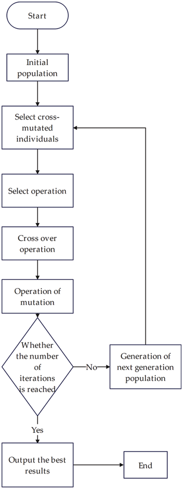
Figure 1: Flow chart of genetic algorithm implementation

3  Enhanced Soft Subspace Clustering Algorithm Based on Genetic Algorithm Optimization

Traditional soft subspace clustering often falls into the local optimum of the algorithm because it relies on the initialized clustering center. By introducing the intelligent population optimization algorithm, the genetic algorithm presented in this paper can obtain an optimal clustering center after the selection, crossover and variation for the clustering center, which effectively resolves the problem of the algorithm falling into the local optimum.

Second, to reduce the susceptibility of soft subspace clustering to noise in the clustering process, MR images usually contain a variety of random noise. Then, generalized noise techniques are introduced in the objective function for weight release constraints to improve the clustering effect of existing algorithms. In this paper, based on the above idea, an enhanced soft subspace clustering algorithm based on genetic algorithm optimization (GAESSCND) is presented.

The advantage of the enhanced soft subspace clustering algorithm based on genetic algorithm optimization is that it can make full use of the data in the soft subspace to assign different weighting coefficients, weaken the initial clustering center through the problem of the global search strategy of the genetic algorithm, and apply it to soft subspace clustering. The optimal solution is obtained through multiple iterations. Additionally, the algorithm optimizes the weights by directly normalizing it to the weights and releasing the weight constraints. Finally, it converges to the local optimal solution. In addition, to solve the boundary segmentation errors of MR images while reducing the noise data for algorithm performance, the generalized noise treatment technique is introduced.

3.1 Objective Function Method Design

Inspired by some ESSC algorithms, exponential coefficients are introduced to fit the given clustering task when performing soft subspace clustering by enhancing intracluster tightness and intercluster separation, and the penalty term is chosen with the same entropy weighting. In addition, the generalized noise clustering algorithm is introduced to reduce the impact of noisy data on the performance of the algorithm. To simplify the objective function and not affect the performance of the algorithm, when the objective function fusion genetic algorithm further optimizes the equality constraint condition of the weight into a bound constraint, the objective function is changed, the iterative formula of the weight is released, and it is integrated into the intraclass similarity and interclass separability. The weight W is directly normalized [44] in the objective function, and the original weight allocation is not the amount of data in the subspace where each cluster is used to ensure that each weight has a nonzero value. The processing formula is shown in Eq. (9) as follows:

∑k=1D(Wik∑k′=1DWik′)=1(9)

Based on the above Eq. (9), we modified the weight part and obtained the objective function Eq. (10) of this paper as follows:

JGAESSCND(U,V,W)=∑i=1C∑j=1NUijm∑k=1D(Wik∑k′=1DWik′)β[ (Xjk−Vik)2−η(Vik−Vok)2 ]         +γ∑i=1C∑k=1D(Wik∑k′=1DWik¢)βln(Wik∑k′=1DWik′)β+∑j=1Nδij2(1-∑i=1CUij)m s.t. Uij∈{ 0,1 }, 0  <  ∑j=1NUij <  1,0  ≤  Wik  ≤  1,  and  ∑k=1DWik=1(10)

The subject of the first soft subspace cluster in the above formula introduces spatial information, including the fuzzy weighting of each sample point and the cluster center. For the weighted distance between each cluster center and the global center, η is the balance factor used to adjust the intraclass similarity and interclass separation. The value range of η is 1, 2, 5, 10, 50, 100, 1000. (Xjk−Vik)2 refers to the Euclidean distance from the jth data point on the kth dimension to the ith cluster class center. Vok  refers to the center of the entire space, and enhances the tightness between classes and the degree of separation between classes by introducing spatial information. The second term is the entropy weighted term, and through the control of the entropy term, the correlation properties found by the soft subspace clustering algorithm belong to the whole dataset not to a specific cluster we need, where the sensitivity of β control weight is; the value range of β, is 1.01, 1.05, 1.2, 1.5, 2, 5, 10, 20, 80, 100. The third item includes the generalized noise technology, which reduces the influence of noise factors through the control of noise data. Other parameters: C refers to the number of clusters; N refers to the total number of data; Uij refers to the membership of the j data point belonging to the i cluster class; m refers to the fuzzy coefficient; the entropy term is controlled by γ, and the proportion of entropy terms in the objective function is controlled by the size of γ; the value range of γ is 0.01, 0.05, 0.1, 0.2, 0.3, 0.5, 0.7, 0.9. In Eq. (10), s.t. is the constraint of the objective function, and after introducing the Lagrange multiplier method, we find the iterative formula of the membership Uij, and the center Vik of the cluster class. λ is generally set at 0.1. The formula for δij2 is Eq. (11) as follows:

δij2=λC×N∑k=1D(Wik∑k′=1DWik′)β∑i=1C∑j=1N[ (Xjk−Vik)2−η(Vik−Vok)2 ](11)

Eq. (11) is the method of calculating the noise distance in noise clustering. The objective function incorporates the ESSC and GNC algorithms to ensure soft subspace clustering while improving the noise immunity of the algorithm. In addition, the points in the original algorithm are retained, the equality constraint of the weight is relaxed into a boundary constraint, and the extreme value is found by the Lagrange multiplier method, leading to the variable membership, Uij, and the cluster center, Vik. The membership method is calculated by Eq. (12) as follows:

Uij={ ∑k=1D(Wik∑k′=1DWik')β[ (Xjk−Vik)2−η(Vik−Vok)2 ] }−1m−1{ ∑i′=1C{ ∑k=1D(Wik∑k′=1DWik')β[ (Xjk−Vik)2−η(Vik−Vok)2 ] } }−1m−1+{ λC × N∑k=1D(Wik∑k′=1DWik')β∑i=1C∑j=1N[ (Xjk-Vik)2- η(Vik-Vok)2 ] }−1m−1(12)

By simplifying the distance formula containing spatial information, we can obtain Dij, which represents the distance between the jth data point on the kth dimension and the ith cluster center minus the distance between each cluster center and the whole space center. Its formula is shown in Eq. (13) as follows:

Dij=[(Xjk−Vik)2−η(Vik−Vok)2](13)

Thus, the formula for calculating the distance is replaced, and the new membership formula obtained is Eq. (14) as follows:

Uij=[ ∑k=1D(Wik∑k′=1DWik′)βDij ]-1m-1{ ∑ik=1C[ ∑k=1D(Wik∑k′=1DWik')βDij ] }-1m-1 +   [ λC × N∑k=1D(Wik∑k′=1DWik′)β∑i=1C∑j=1NDij ] -1m-1(14)

The iterative formula of the clustering center is Eq. (15) as follows:

Vik=∑j=1NUijm(Xjk−ηVOk)∑j=1NUijm(1−η)(15)

After normalizing the weight W directly in the objective function, the objective function fusion genetic algorithm will further optimize the equation constraints of the weight as a boundary constraint. Through the global searchability of the genetic algorithm, the weight matrix W of the algorithm is used as the solution to the problem, and the weight matrix of the t class is Wik. Wik is the solution in the t iteration, while also retaining the corresponding cluster center V and membership U for each Wik. Through constant updating, the update of weight W is completed through the search strategy of the genetic algorithm, while the update formula of Uij and Vik is iterated through the algorithm.

The GAESSCND algorithm is an extension of fuzzy clustering. By adding the penalty term of entropy weighting to regulate the clustering effect, it gradually adjusts the hard clustering to the fuzzy clustering method by introducing spatial information, thus enhancing the effect within the class and paying attention to the information between the classes so that the clustering effect is closer to the actual clustering effect.

3.2 GAESSCND Algorithm and Process

Input: sample size N, data dimension D, number of Clusters C, the maximum number of iterations MaxIter. We set the genetic initialization crossover probability, Pc0, initial variation probability, Pm0, number of generations of the genetic evolution, T, and genetic stopping threshold, δ.

Output: the optimal solution corresponding to U, V, W.

Step 1: Initialization

(1) Set the genetic algebra t = 0 and the fuzzy clustering algebra k = 0. Randomly generate n clustering center matrices to form the initial population:P(t)={Vk(t)|h=0,1,…,n}.

(2) Calculate the number of individuals in the population for each individual f(U,V),f(j),fc(t),fm(t).

(3) The t generation population was selected, crossed and mutated to form the t + 1 generation population.

(4) f(U,V)¯=1n∑k=1nf(k), if t > 0,|f(t)¯−f(t−1)¯|>δ or t < T, then t = t + 1; otherwise, return to Step (2).

(5) Decode and output the cluster center matrix, V(0).

(6) Initialize the weight matrix, W(0)=[Wik]C×D=[1D]C×D, and initialize the affiliation matrix and the objective function.

Step 2: Set the number of iterations t = 0.

Step 3:

For each cluster center:

(1) Calculate Eq. (11).

(2) Calculate the affiliation degree U according to Eq. (14).

(3) Calculate the cluster center V according to Eq. (15).

(4) Calculate the objective function J according to Eq. (10).

(5) Keep executing the above iterative process until the loop reaches the maximum or

END FOR

Step 4: t < maxIter or J>Jmin, go to Step 3; otherwise, go to Step 5.

Step 5: Output U, V. End of algorithm.

The algorithm flow chart is shown in Fig. 2.

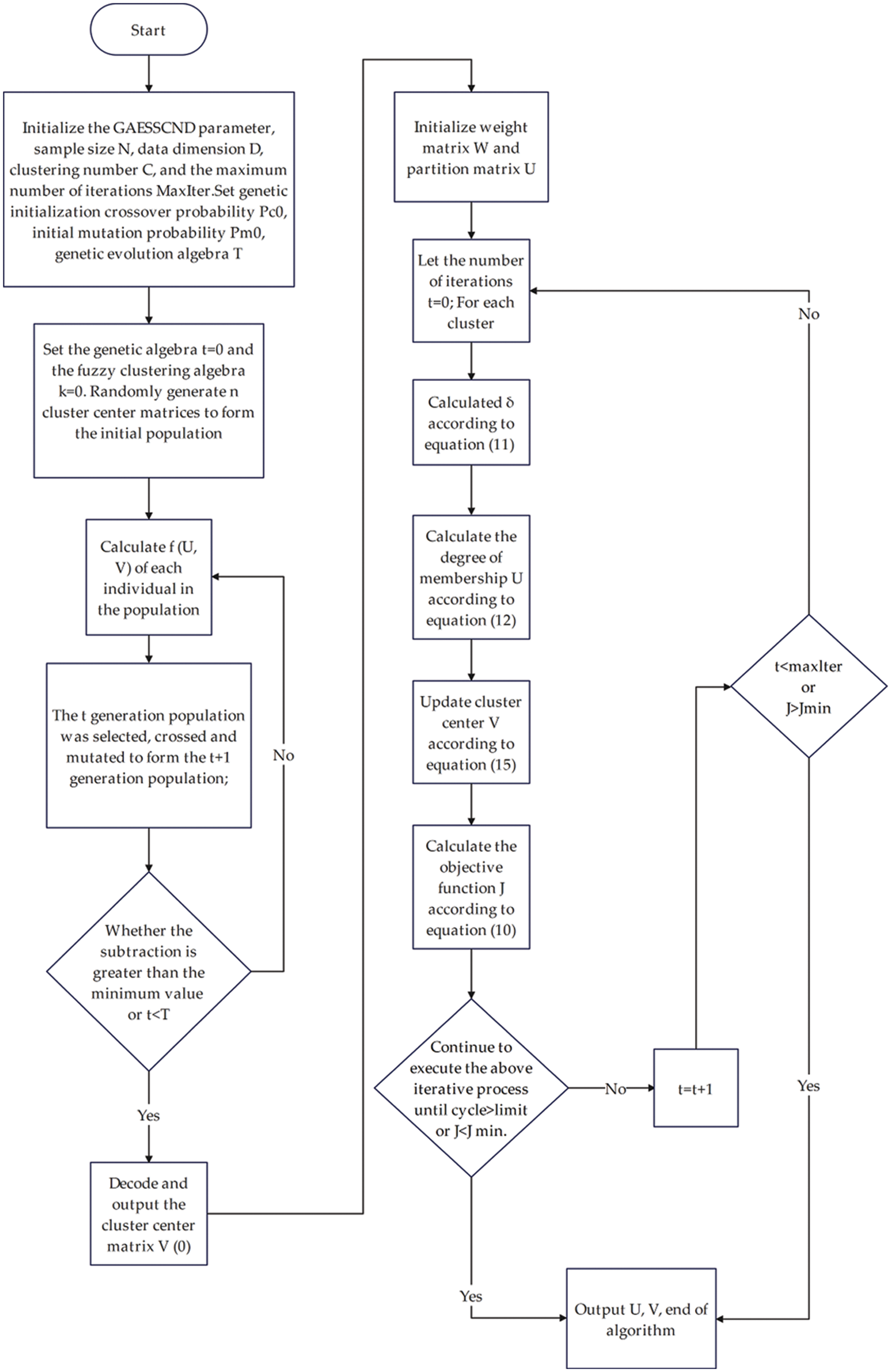
Figure 2: Algorithm flow chart of GAESSCND

4  Experiment

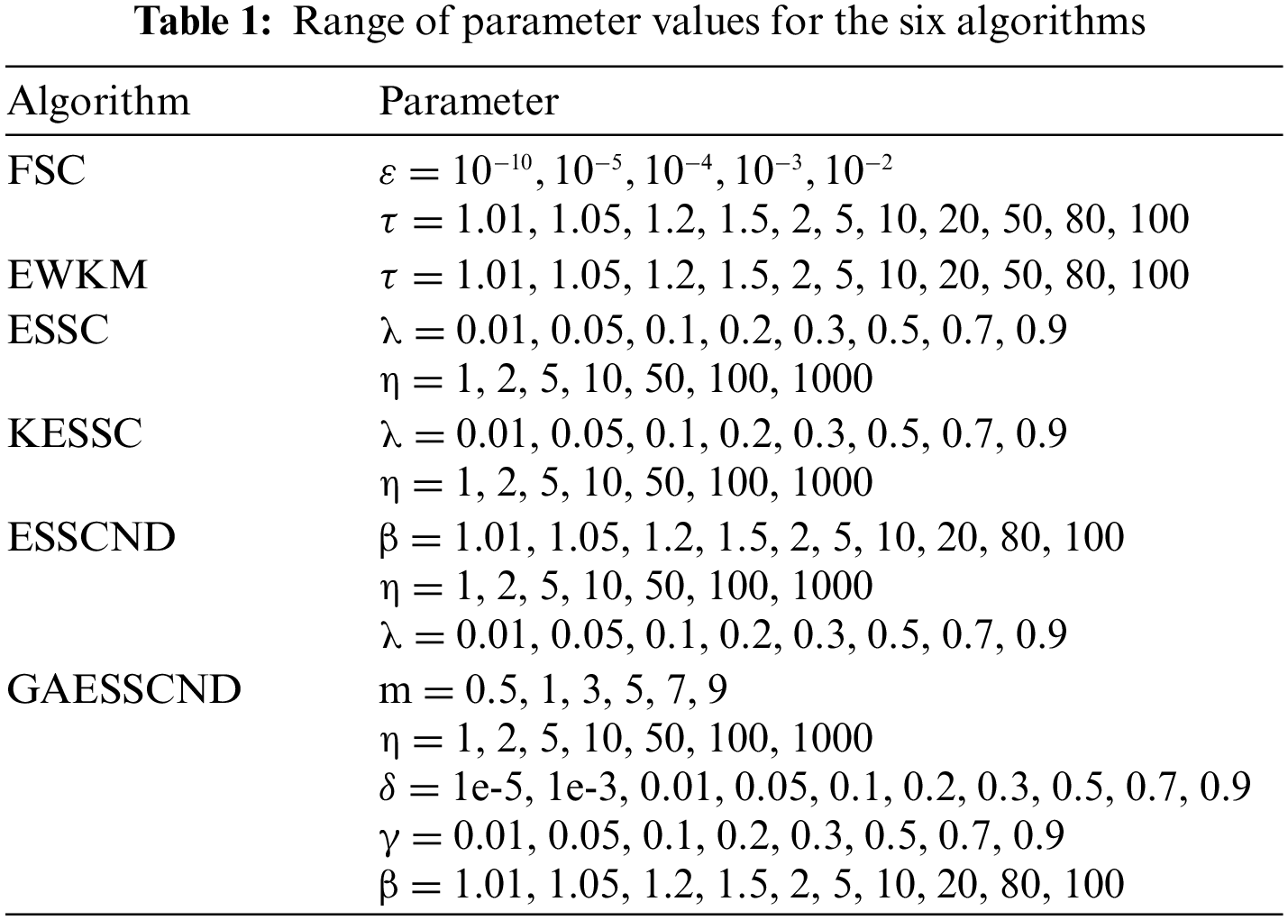
The genetic algorithm is combined to optimize the initial clustering center, and the generalized noise processing technique is introduced to enhance the noise immunity of the algorithm. To verify the performance of the algorithm, the images with the highest noise content are selected in the open-source dataset, and the real provided medical images are experimented on separately. The anti-noise performance of the algorithm is verified by adding noise in real medical images and compared with the traditional soft subspace clustering: EWKM, FSC, ESSC, and the optimized soft subspace clustering algorithms, such as ESSCND and KESSC. In this subsection, publicly available datasets are used to verify the clustering effect of this algorithm on open-source brain datasets and compare it with EWKM, FSC, KESSC, ESSCND and ESSC. The KESSC algorithm introduces kernel space to allocate high-dimensional data in kernel space; the ESSCND algorithm is the randomized initial cluster center and is compared with the genetic algorithm. The parameter ranges in each algorithm are shown in Table 1.

4.1 Experiment on the Segmentation of Publicly Available Brain MR Images

This subsection conducts experiments using publicly available datasets to validate the clustering effect of this paper’s algorithm on top of open-source brain datasets and compare it with the EWKM, FSC, KESSC, ESSCND, and ESSC algorithms. The KESSC algorithm introduces the kernel space to allocate high-dimensional data in the kernel space; the ESSCND algorithm is the randomized initial cluster center and is compared with the genetic algorithm.

The publicly available dataset is derived from the Brain Web countershock brain MR image database of the Brain Imaging Center at the Montreal Neurological Institute of McGill University. The database contains simulated brain MRI data based on two anatomical models, normal and multiple sclerosis (MS), and provides synthetic 3D brain MR images in three modalities (T1-, T2-, PD-). The images contain different scan thicknesses, noise, and offset fields, and the database provides standard segmentation results for all brain MR images.

The experimental platform and environment were as follows: the operating system was macOS; the processor was Apple M1; the compilation environment was MATLAB2021a.

Taking the normal brain database as an example, multiple noise levels were provided, and the noise level pn0 = 0%, 1%, 3%, 5%, 7%, 9%. To verify the anti-noise performance of the algorithm, the highest noise level was selected, and 5 brain images were selected to verify the segmentation effect of the algorithm compared with other soft subspace clustering algorithms. The mode = T1, protocol = ICBM, phantom name = normal, section thickness = 1 mm, noise = 9%, and INU = 0%; brain images of 62 pages, 75 pages, 83 pages, 96 pages, 107 pages were selected. Cluster segmentation was performed for 0 = Background, 1 = CSF, Cerebrospinal Fluid, 2 = Gray Matter, and 3 = White Matter. The effect of segmentation and clustering is shown in Fig. 3:

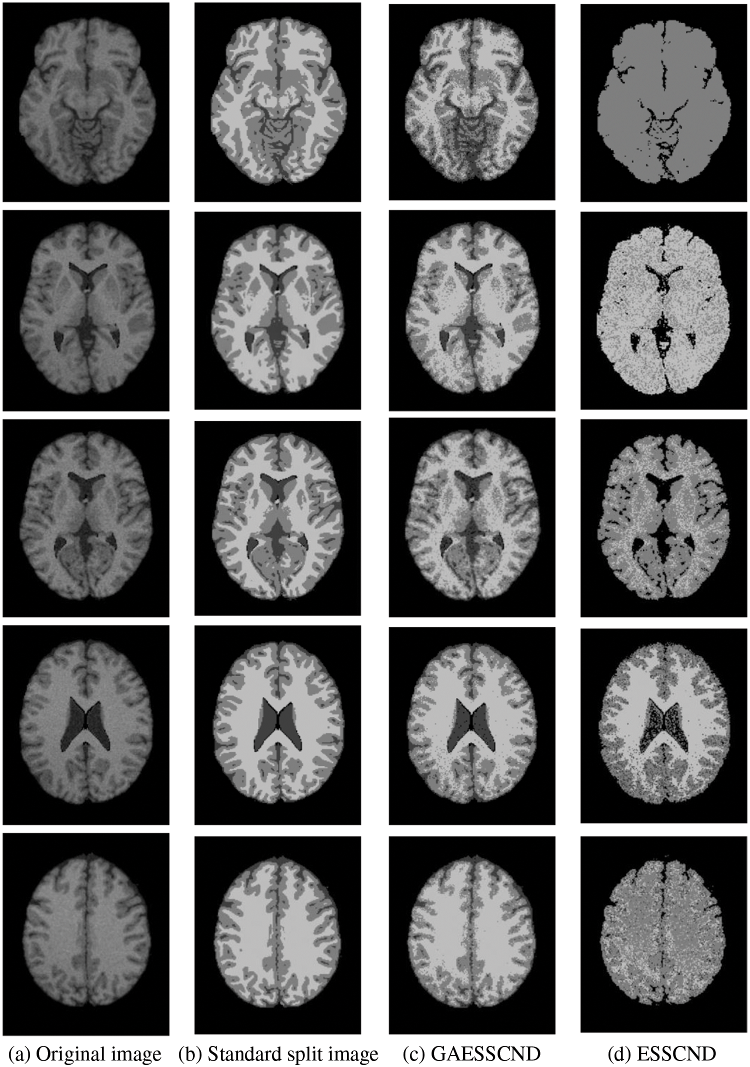
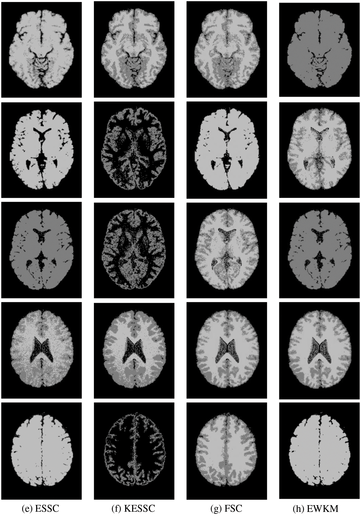
Figure 3: The segmentation result of the T1-weighted simulated brain MR image, (a) depicts the original image, (b) depicts the standard segmentation result graph for evaluation calculation, (c) depicts the segmentation effect of the GAESSCND algorithm proposed in this paper, (d) depicts the segmentation effect of the ESSCND algorithm, (e) depicts the segmentation effect of the ESSC algorithm, (f) depicts the segmentation effect of the KESSC algorithm that guides the kernel function, (g) depicts the segmentation effect of the FSC algorithm, and (h) depicts the segmentation effect of the entropy weighted EWKM algorithm

In Fig. 3, Column (a) is the clustering algorithm proposed in this paper, and the segmentation effect is obviously better than that of other soft subspace clustering algorithms (b–h). In this chapter, the Rand Index (RI) [45], normalized mutual information (NMI) [46] and accuracy indices are used to evaluate the clustering effect, where RI and NMI are calculated by Eqs. (16) and (17), respectively.

RI=(f00+f11)(N(N−1)2)(16)

NMI=∑i=1K∑j=1Cnijlog⁡(Nnijninj){[∑i=1Knilog⁡(niN)][∑j=1Cnjlog⁡(njN)]}12(17)

where K is the total number of labels, C is the number of clusters, N is the total number of samples, f00 represents the sample logarithm of points with different labels assigned to various clusters, f11 represents the sample logarithm of points with the same labels assigned to the same cluster, ni represents the number of samples with the ith label, nj represents the number of samples in Cluster j, and nij represents the logarithm of samples assigned to Cluster j by the sample points with the ith label. The values of RI, NMI and accuracy are all within the interval of [0,1]. The closer the result value is to 1, the better the clustering effect will be.

The RI, NMI and accuracy indices obtained after the corresponding segmentation for each algorithm are given in Table 2 below.

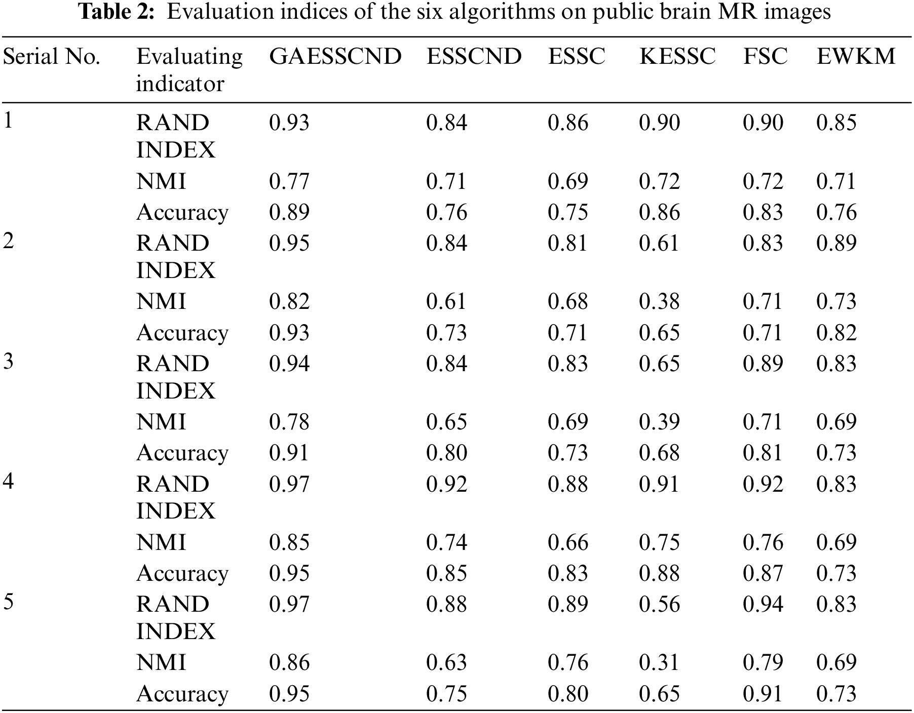
Comparing the data obtained from Table 2, the segmentation effect of the GAESSCND algorithm is very similar to the standard segmentation. The GAESSCND algorithm proposed in this section is compared with four existing soft subspace clustering algorithms, ESSC, EWKM, FSC, and KESSC with a kernel function, and ESSCND with generalized noise detection, where the FSC algorithm is a fuzzy weighted soft subspace clustering algorithm and the EWKM algorithm is an entropy weighted soft subspace clustering algorithm. The ESSC algorithm combines intraclass and interclass information, and the rest of the improved soft subspace clustering algorithms select reasonable parameters in a larger range. The evaluation indices are chosen in 3 ways to determine the noise immunity of the GAESSCND algorithm for noisy MR images. From the displayed visual effect and the 3 evaluation indices, GAESSCND has good noise immunity, and the clustering effect is similar to the standard segmentation. Compared with other soft subspace clustering algorithms, which are not effective in segmenting boundaries and dividing brain regions, the GAESSCND algorithm can clearly divide brain white matter, brain gray matter, cerebrospinal fluid [47] and background regions well so that the problem of noise in MR images of the brain can be handled well.

4.2 Experiment on Segmentation of Real Brain MR Images

For the experiments in the previous subsection, experiments were conducted on publicly available medical brain MR images. In this chapter, the brain MR images provided by the imaging department of the First People’s Hospital of Changshu, Suzhou, China, were selected. In Fig. 4, (a) is the original image provided by the hospital, and the data were acquired by a Philips 3.0T standard MRI scanner with a 3D T1-weighted gradient echo sequence map. The parameters during scanning were as follows: TR = 5.5 ms, TE = 2.7 ms, layer spacing 0.3 mm, layer thickness 1.3 mm, FOV = 35 cm × 35 cm, image size 200 × 200 pixels, and each scan time was 60 s. In this paper, MR images of the clinical brain are used for experiments, and a variety of soft subspace clustering algorithms are used for comparison. The segmentation effect is shown in Fig. 4.

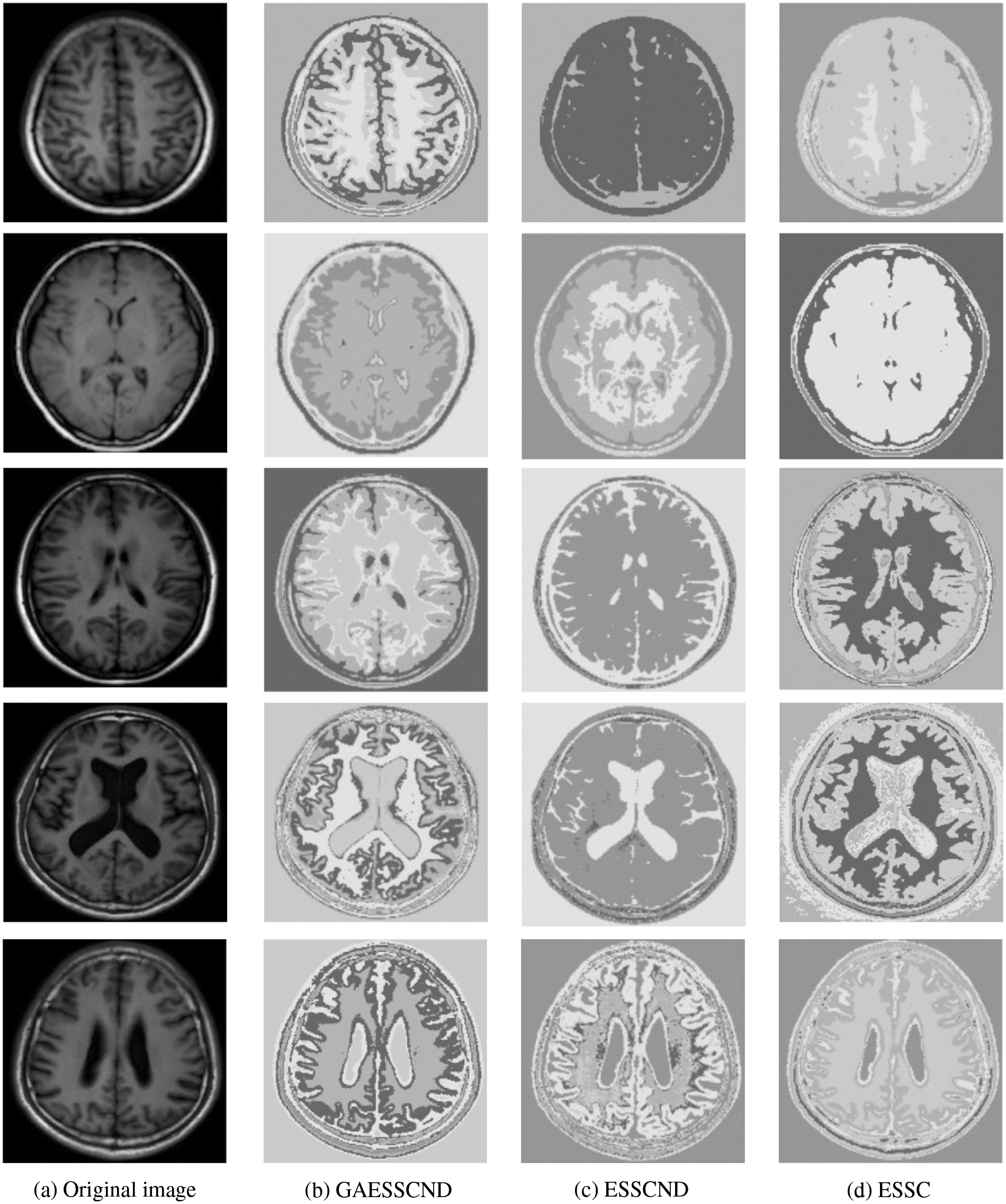
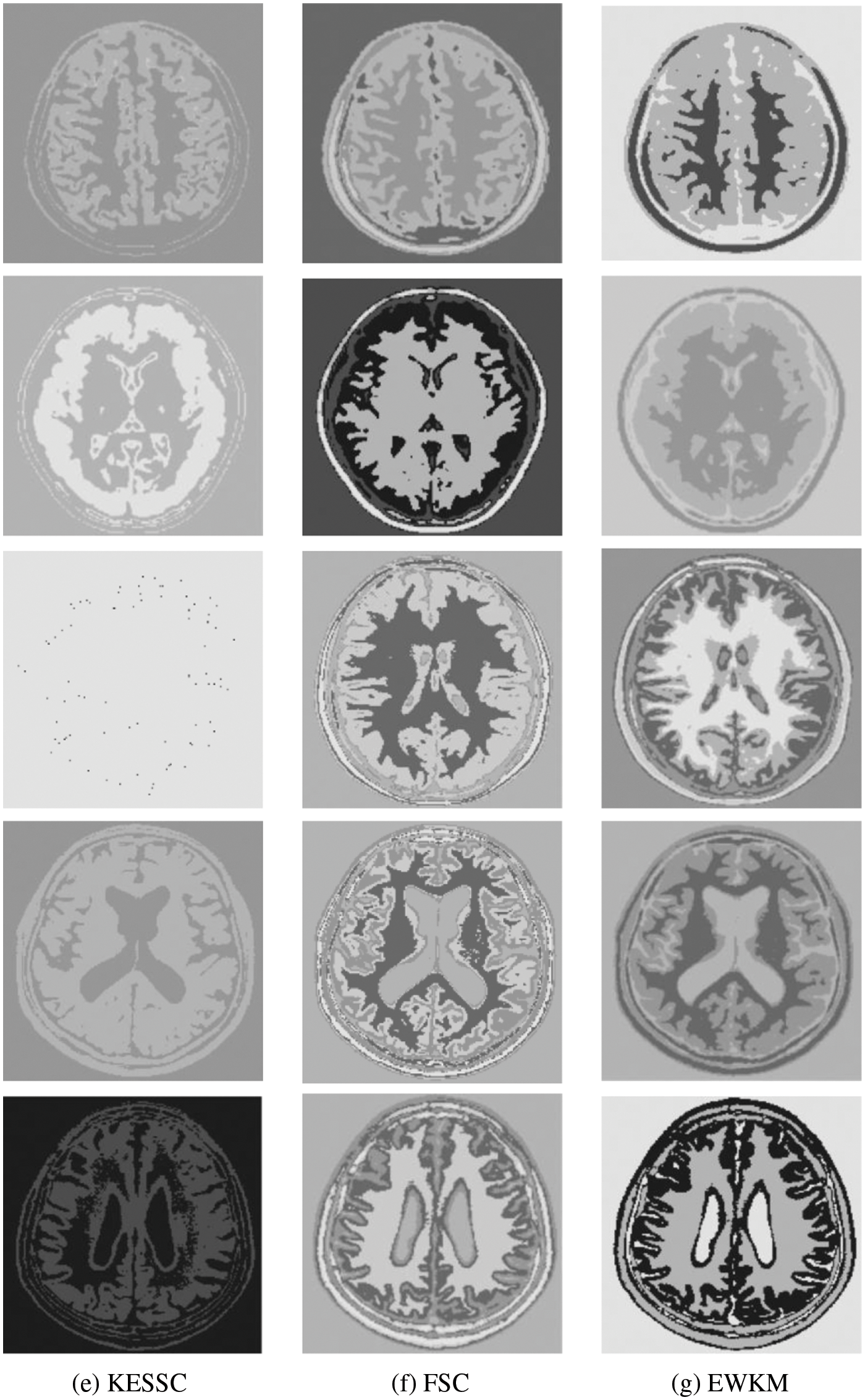
Figure 4: (a) shows the real brain MR image provided by the hospital, (b) shows the segmentation effect of the proposed algorithm, (c) shows the segmentation effect of the ESSCND algorithm, (d) shows the segmentation effect of the ESSC algorithm, (e) shows the segmentation effect of the KESSC algorithm, (f) shows the segmentation effect of the FSC algorithm, and (g) shows the segmentation effect of the EWKM algorithm

The second row in Fig. 4 is the real MR image provided by the hospital, and the image contains 5 classes: 0 = Background, 1 = CSF (cerebrospinal fluid), 2 = Gray Matter, 3 = White Matter, and 4 = Skull; these 5 classes are segmented by clustering segmentation. Table 2 shows that the GAESSCND algorithm is able to segment the 5 classes with clear boundaries, while the rest of the comparison algorithms have poor results in the face of noise processing, with mixed boundaries and mis-segmented brain tissue.

Due to the lack of truth maps in the dataset provided by the hospital, the evaluation metrics were chosen from the internal evaluation metrics in MATLAB. Davies–Bouldin index (DBI) [48] silhouette coefficient (SC) [49].

The meaning of DBI is the mean value of the maximum similarity of each cluster class; the smaller the value of DBI is, the better the clustering effect. Its calculation formula is shown in Eq. (18) as follows:

DBI=1N∑i=1Nmaxj≠i(Si¯+Sj¯||Wi−Wj||2)(18)

SC: represents the formula contour coefficient; the larger the contour coefficient is, the better the clustering effect. Its calculation formula is shown in Eq. (20) as follows:

S(i)=b(i)−a(i)max(a(i),b(i)),if|Ci|>1(19)

SC=maxks¯(k)(20)

In Table 3, it can be seen that the proposed GAESSCND algorithm segmentation yields the best results with the smallest DBI coefficient, the strongest similarity in each cluster class, and the largest contour coefficient SC, segmenting significantly and outperforming other clustering algorithms. In the experimental process of Fig. 3, the KESSC algorithm has most of the kernel space with zero, resulting in obvious deviation of the weight contribution; the experimental segmentation effect is poor, and the corresponding evaluation index result is NaN.

Because in the MR imaging process, the real and imaginary parts of the signal are disturbed by Gaussian noise with uncorrelated zero mean and the same variance at the same time due to the influence of environment and equipment, in order to verify the anti-noise property of GAESSCND, the noise addition process is performed again for the image to simulate the problems of blurred boundary and poor visual effect after the MR image is subjected to noise by adding speckle noise to the image provided by the hospital, taking the value of 0.03. By comparing the experiment with other soft subspace clustering, the segmentation effect obtained is shown in Fig. 5.

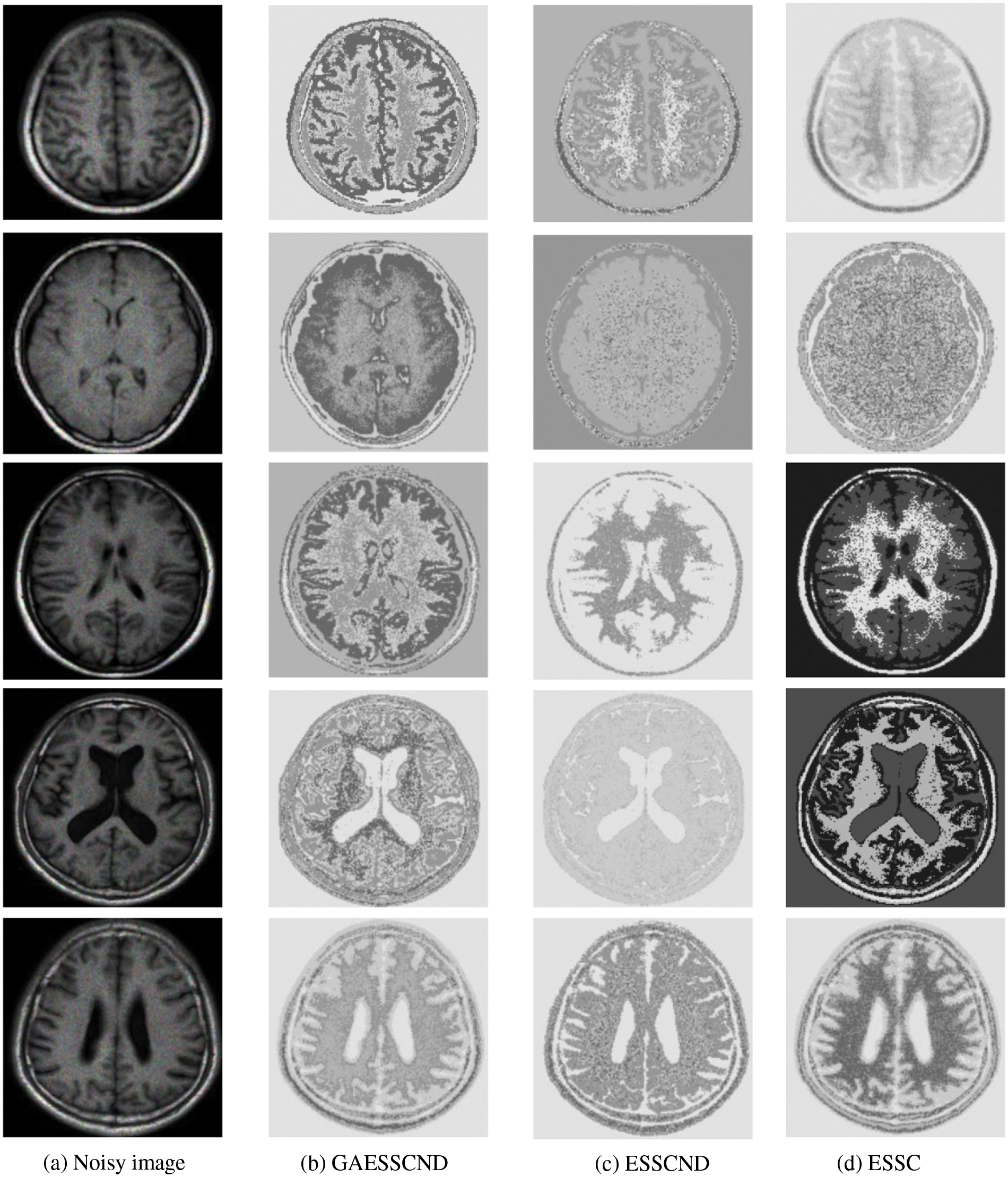
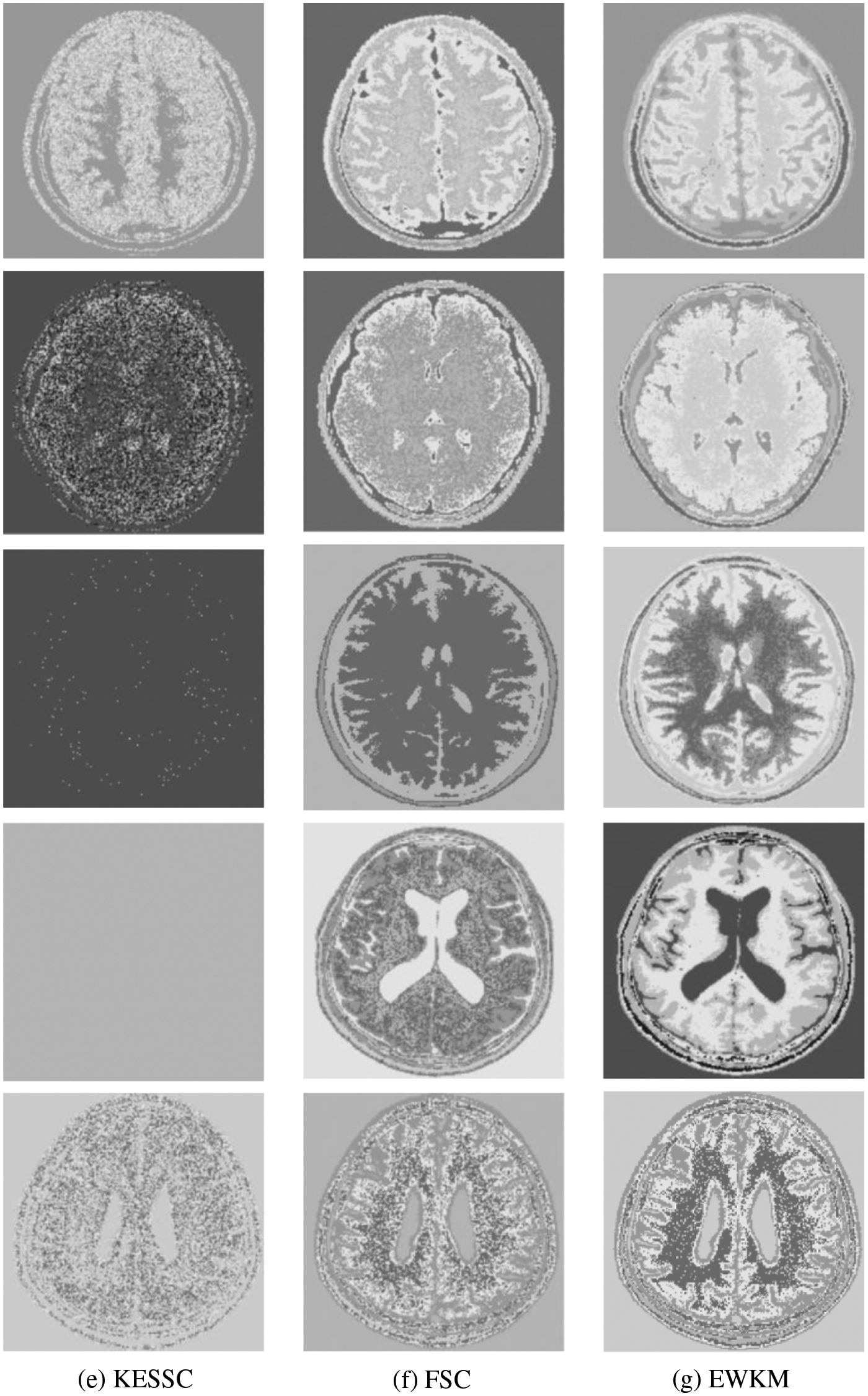
Figure 5: (a) Depicts the hospital brain MR image after noise, (b) is the segmentation effect of the proposed algorithm, (c) is the segmentation effect of the ESSCND algorithm, (d) is the segmentation effect of the ESSC algorithm, (e) is the segmentation effect of the KESSC algorithm, (f) is the segmentation effect of the FSC algorithm, and (g) is the segmentation effect of the EWKM algorithm

The experimental data are shown in Table 4 below.

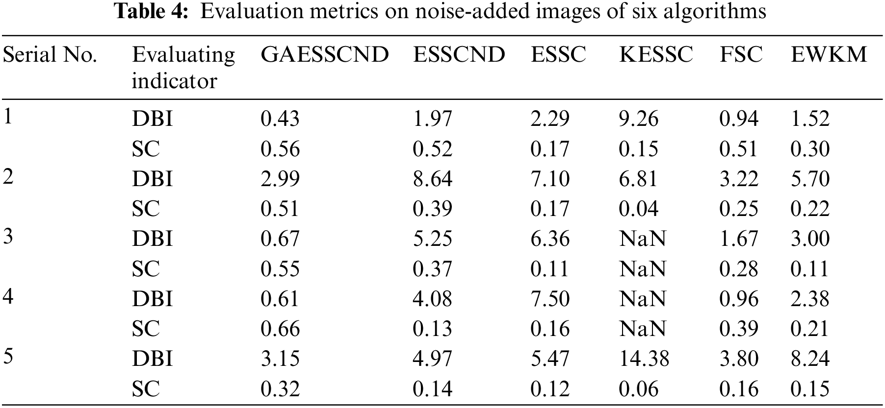
Through the experiments, (a) in Fig. 3 is the image after noise, and the (b–g) columns are all the effects after clustering segmentation of the brain MR containing noise. From a visual perspective, the GAESSCND algorithm has the strong anti-noise ability, among which KESSC has segmentation failure for serial numbers 3 and 4 and cannot segment the brain tissues in the images containing noise. Under the influence of noise, KESSC affects the weight allocation in nuclear space, most of which has zero weight. After the cluster center and membership fall into the local optimal solution in the iteration, the experimental results are wrong, and the brain tissue cannot be segmented from the image containing noise. KESSC is also more suitable for high-dimensional datasets and does not have a good processing advantage for noisy data. From the experimental data obtained in Table 4, it can be seen that GSESSCND shows very good results for all five noise-added brain MR images. The rest of the soft subspace clustering shows insufficient noise immunity for the images with noise, and the brain MR images are segmented incorrectly.

Finally, the GAESSCND algorithm showed good clustering results for both hospital-supplied MR images and noise-added images, reflecting the robustness and noise resistance of the algorithm. From some of the compared soft subspace clustering algorithms, the rest of the soft subspace clustering showed unclear boundary segmentation, high noise content, and unclear soft tissue segmentation.

The time complexity of the GAESSCND algorithm is correlated to the number of data, dimension and number of clusters. The time complexity of the membership calculation is related to the amount of data, N, cluster number C and sample dimension D, and its time complexity is O (NCD). The dimension weight calculation is related to the number of clusters and the sample dimension, and its time complexity is O (CD). The time complexity of the generalized noise clustering is related to the number of clusters, N, and the sample dimension, C, and its time complexity is O (NC). Introducing a genetic algorithm into the clustering process, its time complexity is related to the amount of data, N, and the number of iterations, T, and its time complexity is O (TN). The three are peers in the computer execution process, and T>CN. Therefore, the time complexity of GAESSCND proposed in this paper is O (TN). The introduction of the optimization algorithm makes the running time of this algorithm higher than that of EWKM, FSC, ESSC, KESSC and ESSCND. If the real-time requirement is not very high, it is important to exchange a relatively long time for a higher image segmentation accuracy.

5  Conclusion

In this paper, a soft subspace clustering algorithm for brain MR images based on genetic algorithm optimization is proposed. To improve the noise clustering performance, the algorithm first introduces the generalized noise clustering function into the objective function and chooses the genetic algorithm strategy to optimize the affiliation calculation method to find the subspace where the cluster classes are located when initializing the clustering centers; the weight constraints are released in the objective function and normalized in the objective function directly; the similarity between each class is maximized by enhancing the intraclass tightness and interclass separation. In addition, the algorithm avoids the problem of falling into a local optimum, effectively weighs the local and global searchability, and improves the clustering effect for the boundary.

This paper verifies the effectiveness of the GAESSCND algorithm by performing two experiments, which also presents new progress to the research of medical images. For doctors’ diagnoses, when an MR image containing noise is obtained by the influence of the external environment, the lesion may be together with normal tissue at this time, which may easily cause brain tissue segmentation errors, and the boundary of the image containing noise will become blurred when clustering. It is easy to misclassify the lesion area at this time, so noise immunity plays a crucial role in medical images.

Finally, the proposed algorithm for noisy images has a good segmentation effect for medical images and other images containing noise. However, the algorithm still has some defects, and the experimental results are unstable. The emergence of this problem is because the main framework of the algorithm is still based on the soft subspace clustering algorithm. Once in the initial clustering center into the local optimal influence, the experimental results will appear unstable, and adding a genetic algorithm can only optimize and cannot completely solve the problem of soft subspace clustering itself. In the future, the algorithm should focus on a variety of different frameworks, combining the knowledge of deep learning to optimize the clustering algorithm itself, which will produce better segmentation results.

Funding Statement: This work was supported in part by the National Natural Science Foundation of China under Grant 62171203, in part by the Suzhou Key Supporting Subjects [Health Informatics (No. SZFCXK202147)], in part by the Changshu Science and Technology Program [No. CS202015, CS202246], in part by the Changshu City Health and Health Committee Science and Technology Program [No. csws201913], and in part by the “333 High Level Personnel Training Project of Jiangsu Province”.

Conflicts of Interest: The authors declare that they have no conflicts of interest to report regarding the present study.

References

1. Tonozuka, R., Mukai, S., Itoi, T. (2020). The role of artificial intelligence in endoscopic ultrasound for pancreatic disorders. Diagnostics, 11(1), 18. https://doi.org/10.3390/diagnostics11010018 [Google Scholar] [PubMed] [CrossRef]

2. Lalchhanhima, R., Saha, G., Nunsanga, M., Kandar, D. (2020). Synthetic aperture radar image segmentation using supervised artificial neural network. Multiagent and Grid Systems, 16(4), 397–408. [Google Scholar]

3. Kong, H., Kang, Q., Li, W., Liu, C., He, H. (2019). A hybrid iterated carousel greedy algorithm for community detection in complex networks. Physica A: Statistical Mechanics and its Applications, 536, 122124. [Google Scholar]

4. McKenzie, F., Zietsman, A., Galukande, M., McCormack, V. (2018). Drivers of advanced stage at breast cancer diagnosis in the multicountry African breast cancer—disparities in outcomes (ABC-DO) study. International Journal of Cancer, 142(8), 1568–1579. [Google Scholar] [PubMed]

5. Dimitriadis, A., Trivizakis, E., Papanikolaou, N., Tsiknakis, M., Marias, K. (2022). Enhancing cancer differentiation with synthetic MRI examinations via generative models: A systematic review. Insights into Imaging, 13(1), 1–27. [Google Scholar]

6. Wang, S. H. (2021). COVID-19 classification by CCSHNet with deep fusion using transfer learning and discriminant correlation analysis. Information Fusion, 68(1), 131–148. [Google Scholar] [PubMed]

7. Singh, S., Srivastava, S. (2022). Kernel fuzzy C-means clustering with teaching learning based optimization algorithm (TLBO-KFCM). Journal of Intelligent & Fuzzy Systems, 42(1), 1–9. [Google Scholar]

8. Li, E., Zeng, X. Y. (2021). Evaluating the performance of fine bubble diffused aeration systems in cylindrical aeration tanks by fuzzy c-means algorithm. Water Science and Technology, 84(2), 404–419. [Google Scholar] [PubMed]

9. Agrawal, R., Gehrke, J. E., Gunopulos, D., Raghavan, P. (1998). Automatic subspace clustering of high dimensional data for data mining applications. ACM SIGMOD Record, 27(2), 94–105. [Google Scholar]

10. Zhao, K. F., Jiang, Y. Z., Xia, K. J., Qian, P. J. (2020). View-collaborative fuzzy soft subspace clustering for automatic medical image segmentation. Multimedia Tools and Applications, 79(10), 9523–9542. [Google Scholar]

11. Teng, Y. Y., Qi, S. L., Han, F. F., Xu, L. S., Yao, Y. D. et al. (2021). Two graph-regularized fuzzy subspace clustering methods. Applied Soft Computing Journal, 100, 106981. [Google Scholar]

12. Amorim, R. C. D., Mirkin, B. (2011). Minkowski metric, feature weighting and anomalous cluster initializing in K-Means clustering. Pattern Recognition, 45(3), 1061–1075. [Google Scholar]

13. Xu, Y. J., Wu, X. J. (2016). Soft subspace clustering algorithm based on quantum behavior particle swarm optimization. Pattern Recognition and Artificial Intelligence, 29(6), 558–566. [Google Scholar]

14. Ye, L., Zheng, D., Sui, D., Wu, D. (2022). Artificial colony optimization density peak clustering for high-dimensional data. Journal of Nanjing University of Technology, 46(3), 291–297. [Google Scholar]

15. Li, M., Wang, L. (2022). A soft subspace clustering integration method based on random walk. Journal of Yantai University (Natural Science and Engineering Edition), 35(3), 343–350+370. [Google Scholar]

16. Lin, Z., Lei, J. S., Bi, Z. Q., Yang, J. (2013). A data stream based soft subspace clustering algorithm. Journal of Software Science, 24(11), 2610–2627. [Google Scholar]

17. Fan, H., Shi, X. M., Yao, R. X. (2020). Brainstorming algorithm optimized soft subspace clustering algorithm for breast MR images. Computer Science and Exploration, 14(8), 1348–1357. [Google Scholar]

18. Xiao, J. L., Liu, S. J., Liu, H. T., Wang, M. L., Li, G. X. et al. (2022). A jerk-limited heuristic feedrate scheduling method based on particle swarm optimization for a 5-DOF hybrid robot. Robotics and Computer-Integrated Manufacturing, 78, 102396. [Google Scholar]

19. Kabir, A. M., Kamal, M., Ahmad, F., Ullah, Z., Albogamy, F. R. et al. (2021). Optimized economic load dispatch with multiple fuels and valve-point effects using hybrid genetic-artificial fish swarm algorithm. Sustainability, 13(19), 1–27. [Google Scholar]

20. Ramshanker, A., Isaac, J. R., Jeyeraj, B. E., Swaminathan, J., Kuppan, R. (2022). Optimal DG placement in power systems using a modified flower pollination algorithm. Energies, 15(22), 8516. [Google Scholar]

21. Hc, A., Sl, A., Rmm, B., Aad, C. (2021). Optimization of inflow performance relationship curves for an oil reservoir by genetic algorithm coupled with artificial neural-intelligence networks. Energy Reports, 7, 3116–3124. [Google Scholar]

22. Moura, L., Monteiro, P. P., Darwazeh, I. (2005). Generalized noise analysis technique for four-port linear networks. IEEE Transactions on Circuits and Systems I: Regular Papers, 52(3), 631–640. [Google Scholar]

23. Wang, S. H., Govindaraj, V. V. M. G., Juan, Z., Xin, Z., Yu, D. (2020). COVID-19 classification by FGCNet with deep feature fusion from graph convolutional network and convolutional neural network. Information Fusion, 67(1), 208–229. https://doi.org/10.1016/j.inffus.2020.10.004 [Google Scholar] [PubMed] [CrossRef]

24. Zhu, L., Cao, L., Yang, J., Lei, J. (2014). Evolving soft subspace clustering. Applied Soft Computing Journal, 14, 210–228. https://doi.org/10.1016/j.asoc.2013.03.002 [Google Scholar] [CrossRef]

25. Ni, S. T. (2022). Abnormal-aware multiperson evaluation system with improved fuzzy weighting. Journal of Function Spaces, 2022, 4899831. [Google Scholar]

26. Khan, M., Haj Ismail, A. A. K., Ishaque, I., Hussain, I. (2021). New combination of simple additive and entropy weighting criteria for the selection of best substitution box. Journal of Intelligent and Fuzzy Systems, 41(3), 1–14. https://doi.org/10.3233/JIFS-211176 [Google Scholar] [CrossRef]

27. Chan, E. Y., Ching, W. K., Ng, M. K., Huang, J. Z. (2003). An optimization algorithm for clustering using weighted dissimilarity measures. Pattern Recognition, 37(5), 943–952. [Google Scholar]

28. Upadhyay, D., Jain, S., Jain, A. (2013). A fuzzy clustering algorithm for high dimensional streaming data. Journal of Information Engineering and Applications, 3(10), 1–9. [Google Scholar]

29. Paul, D., Saha, S., Mathew, J. (2020). Improved subspace clustering algorithm using multi-objective framework and subspace optimization. Expert Systems with Applications, 158, 113487. https://doi.org/10.1016/j.eswa.2020.113487 [Google Scholar] [CrossRef]

30. Liu, L., Kuang, L., Ji, Y. (2020). Multimodal MRI brain tumor image segmentation using sparse subspace clustering algorithm. Computational and Mathematical Methods in Medicine, 2020, 1–13. [Google Scholar]

31. Gan, G., Wu, J. (2007). A convergence theorem for the fuzzy subspace clustering (FSC) algorithm. Pattern Recognition, 41(6), 1939–1947. [Google Scholar]

32. Ji, J., Wei, P., Zheng, Y., Zhe, W., Ma, Z. (2015). An initialization method for clustering mixed numeric and categorical data based on the density and distance. International Journal of Pattern Recognition and Artificial Intelligence, 29(7), 150621203409007. [Google Scholar]

33. Zhang, Y. D., Dong, Z., Wang, S. H., Yu, X., Gorriz, J. M. (2020). Advances in multimodal data fusion in neuroimaging: Overview, challenges, and novel orientation. Information Fusion, 64, 149–187. [Google Scholar] [PubMed]

34. Jing, L., Ng, M. K., Huang, J. Z. (2007). An entropy weighting K-means algorithm for subspace clustering of high-dimensional sparse data. IEEE Transactions on Knowledge and Data Engineering, 19(8), 1026–4041. [Google Scholar]

35. Zhang, G. Y., Wang, C. D., Huang, D., Zheng, W. S. (2017). Multi-view collaborative locally adaptive clustering with Minkowski metric. Expert Systems with Applications, 86, 307–320. [Google Scholar]

36. Ydza, B., Scs, C., Dsg, D., Jmg, E., Shwb, F. (2021). Improved breast cancer classification through combining graph convolutional network and convolutional neural network. Information Processing and Management, 58(2), 1–25. [Google Scholar]

37. Chen, Y. T. (2020). Evaluation and analysis of electronic information industry clustering level based on soft subspace clustering algorithm. Journal of Physics: Conference Series, 1533(2), 022052. [Google Scholar]

38. Deng, Z., Choi, K. S., Jiang, Y., Wang, J., Wang, S. (2016). A survey on soft subspace clustering. Information Sciences, 348, 84–106. https://doi.org/10.1016/j.ins.2016.01.101 [Google Scholar] [CrossRef]

39. Zhang, Y. D., Satapathy, S. C., Wu, D., Guttery, D. S., Górriz, J. M. et al. (2020). Improving ductal carcinoma in situ classification by convolutional neural network with exponential linear unit and rank-based weighted pooling. Complex & Intelligent Systems, 7(3), 1295–1310. [Google Scholar]

40. Li, M., Li, W. J., Qiao, J. F. (2022). Design of a modular neural network based on an improved soft subspace clustering algorithm. Expert Systems with Applications, 209, 118219. [Google Scholar]

41. Davé, R. N., Sen, S. (1998). Generalized noise clustering as a robust fuzzy c-M-estimators model. 1998 Conference of the North American Fuzzy Information Processing Society-NAFIPS (Cat. No. 98TH8353), pp. 256–260. Piscataway, IEEE. [Google Scholar]

42. Karthika, R., Revathi, S. (2014). Fuzzy possibilistic C-mean clustering algorithm for text categorization. Fuzzy Systems, 6(3), 75–77. [Google Scholar]

43. Bhavana, D., Rajesh, V., Kishore, P. (2016). A new pixel level image fusion method based on genetic algorithm. Indian Journal of Science and Technology, 9(45), 1–8. [Google Scholar]

44. Lepcha, D. C., Goyal, B., Dogra, A. (2020). Image fusion based on cross bilateral and rolling guidance filter through weight normalization. The Open Neuroimaging Journal, 13(1), 51–61. [Google Scholar]

45. Miin, S. Y., Chiou, C. Y. (2018). Fuzzy generalization and comparisons for the rand index. International Journal of Intelligent Systems, 33(5), 901–927. [Google Scholar]

46. Darong, L., Christine, N. (2016). A corrected normalized mutual information for performance evaluation of community detection. Journal of Statistical Mechanics: Theory and Experiment, 2016(9), 093403. [Google Scholar]

47. Mol, J. R., Rashmi, A. G., Mohan, K. J., Alsaheer, S. S., Mable, A. et al. (2018). A simple and robust strategy for background removal from brain MR images. IOP Conference Series: Materials Science and Engineering, 396(1), 012039. [Google Scholar]

48. Firman, T., Achmad, F. A. (2018). Clustering of potency of shrimp in Indonesia with K-means algorithm and validation of Davies-Bouldin index. Proceedings of the International Conference on Science and Technology, pp. 730–733. Västerås, Sweden, Atlantis Press. [Google Scholar]

49. Zhou, H. B., Gao, J. T. (2014). Automatic method for determining cluster number based on silhouette coefficient. Advanced Materials Research, 951, 227–230. [Google Scholar]