
 Submit a Paper
 Propose a Special lssue
 Open Access
ARTICLE
Nonlinear Analysis of Organic Polymer Solar Cells Using Differential Quadrature Technique with Distinct and Unique Shape Function
1
Department of Engineering Mathematics and Physics, Faculty of Engineering, Zagazig University, Zagazig, 44519, Egypt
2
Basic Science Department, Faculty of Engineering, Delta University for Science and Technology, Gamasa, 11152, Egypt
3
Department of Medical Research, China Medical University Hospital, China Medical University, Taichung, 404327, Taiwan
* Corresponding Author: Omer Civalek. Email:
Computer Modeling in Engineering & Sciences 2023, 137(3), 2193-2217. https://doi.org/10.32604/cmes.2023.028992
Received 22 January 2023; Accepted 23 April 2023; Issue published 03 August 2023
 View Full Text
 Download PDF
Abstract
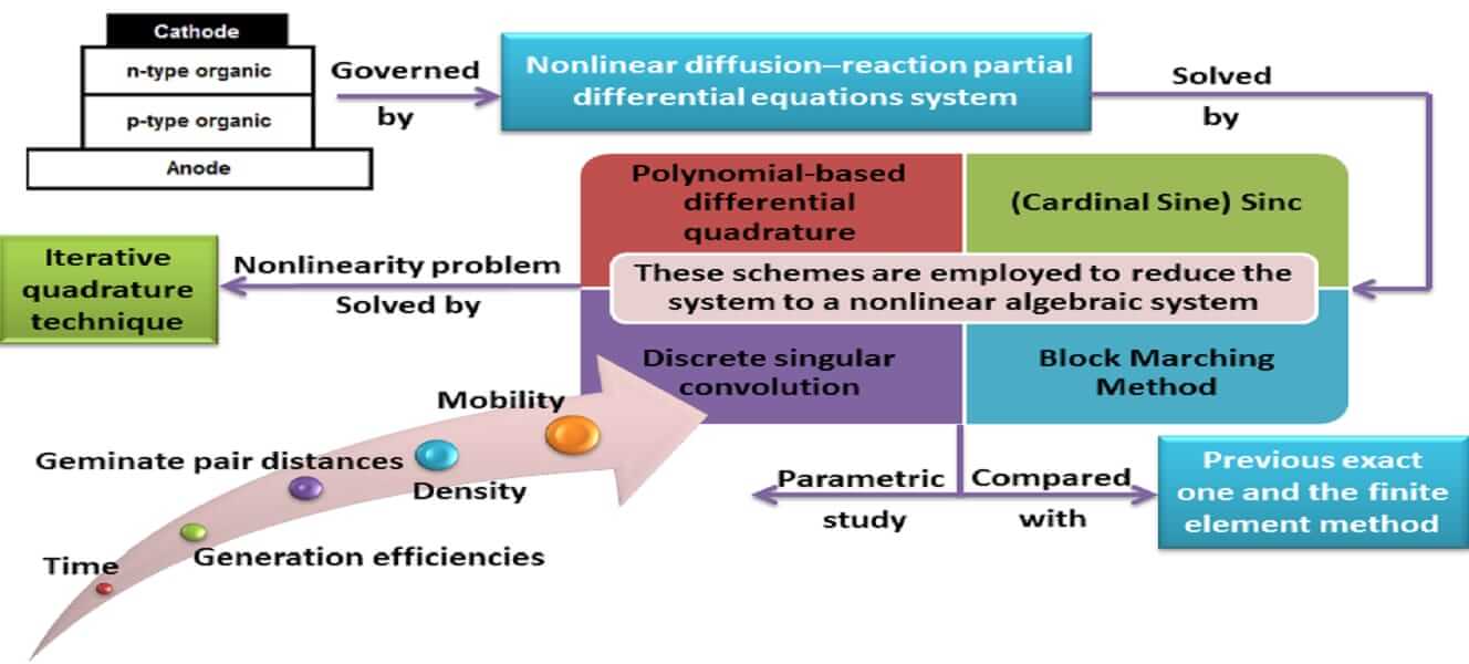
Four numerical schemes are introduced for the analysis of photocurrent transients in organic photovoltaic devices. The mathematical model for organic polymer solar cells contains a nonlinear diffusion–reaction partial differential equation system with electrostatic convection attached to a kinetic ordinary differential equation. To solve the problem, Polynomial-based differential quadrature, Sinc, and Discrete singular convolution are combined with block marching techniques. These schemes are employed to reduce the problem to a nonlinear algebraic system. The iterative quadrature technique is used to solve the reduced problem. The obtained results agreed with the previous exact one and the finite element method. Further, the effects of different times, different mobilities, different densities, different geminate pair distances, different geminate recombination rate constants, different generation efficiencies, and supporting conditions on photocurrent have been analyzed. The novelty of this paper is that these schemes for photocurrent transients in organic polymer solar cells have never been presented before, so the results may be useful for improving the performance of solar cells.Graphic Abstract
Keywords
Nomenclature
| Flux density of electron | |
| Flux density of proton | |
| Total current density | |
| Carrier mobilities for electron and hole | |
| Carrier generation rates for electron and hole | |
| Recombination rates for electron and hole | |
| Charge carrier diffusion coefficients for electron and hole | |
| Elementary charge | |
| Time | |
| Dissociation of charge pairs rate | |
| Charge pairs generation rate | |
| Electron–hole pair binding energy | |
| Pair distance | |
| Relative permittivity of polymer | |
| Permittivity of free space | |
| Boltzmann’s constant | |
| Absolute temperature (300 k) | |
| Bimolecular recombination rate | |
| Monomolecular recombination rate | |
| State effective density | |
| Electron and hole energy barriers | |
| Wave length | |
| Band gap | |
| Applied voltage |
Energy disasters, the release of greenhouse gases, and global warming are known to be some of the most extreme threats to life in the future. Therefore, renewable energy has found great attention from consumer countries to reduce carbon-based energy supplies [1]. One of the renewable energy sources that has attracted great attention from research communities is organic solar cells (OSCs) [2–4].
Third-generation photovoltaic devices [5] divide into two branches: organic polymer cells [6–8] and electrochemical cells [9–11]. We will concern with organic polymer cells in this paper. This type of renewable energy source has numerous advantages, such as low cost of manufacturing [12,13] and easy processing on flexible substrates [14–16]. Bulk-heterojunction (BHJ) structure improves the performance of organic polymer cells where electron donor and acceptor materials are mixed in a solution and cast into a thin film sandwiched between two electrodes [7,8], as shown in Fig. 1. The dynamics of charge behaviors in photovoltaic cells are displayed by measurements of transient photocurrent [17]. The classic time-of-flight technique measures the behavior of charge carriers generated according to a light, short pulse. Carriers are generated beside the electrode to allow extracting mobility and transit time [18,19].

Figure 1: Schematic of a heterojunction organic solar cell with its energy band diagram
Many researchers have examined the design of solar cells experimentally [20], but only a limited number of cases have been solved analytically and numerically. de Falco et al. [21] numerically studied photocurrent transients in organic polymer solar cells using the finite element and Newton-Raphson techniques, and they also produced an analytical solution for the problem. Buxton et al. [22] used the finite difference method to present computer simulations of polymer solar cells. Hwang et al. [23] investigated the photocurrent transients of organic solar cells using numerical simulations of the drift-diffusion formulas. van Mensfoort et al. [24] described two alternative iterative methods for obtaining solutions to the drift-diffusion equation. Koster et al. [25] presented the theory of Braun for showing the temperature and field dependence of the photocurrent in PPV: PCBM blends. However, for such problems, computational ill-conditioning is to be expected [26,27]. El Karkri et al. [28] used one dimension program [AMPS-1D] to optimize the performance of organic solar cells based on (carbazole-methylthiophene), benzothiadiazole and thiophene [(Cbz-Mth)-B-T]2 as electron donors, and [6,6]-phenyl-C61-butyric acid methyl ester (PCBM) as an electron acceptor. Yousuf et al. [29] analyzed the p-type Cu2O layer as a hole transport layer on Cu (In, GA) Se2 (CIGS) absorber layer. The analysis was performed by utilizing the solar cell capacitance simulator, SCAPS-1D. Overall, the solar cell conversion efficiency improved from 18.72% to 26.62% by adding a Cu2O hole transport layer and substituting CdS with ZnSe. Islam [30] investigated the thin-film organic solar cell (OSC) performances in detail by improved analytical computation in this work. The generation of excitons inside OSC has been estimated by using the optical transfer matrix method (OTMM) to include the optical phenomena of the incident light. The effect of mobility and active layer thickness on the properties of bulk heterojunction solar cells was investigated using the drift-diffusion model by Sadoogi et al. [31].
The differential quadrature method (DQM) is able to achieve accurate results without exerting high effort [28]. DQM comes in a variety of versions, each with its own shape function and influence domain for each point. The most used versions are Polynomial (PDQM) [32–34], Sinc (SDQM) [35], and Discrete singular convolution (DSCDQM) [36–44]. Ragb et al. [45–46] studied the performance of composite solar cell model consisting of perovskite absorber layer (CH3NH3PbI3), electron transport layer (TiO2 or PCBM), and hole transport layer (Spiro-OMeTAD or CuI) via sinc and discrete singular convolution quadrature techniques. Also, they presented different numerical methods that are used for the first time in solving Perovskite solar cells (PSCs). Ragb et al. [47] offered Improved electromagnetism-like algorithm and Differential quadrature technique to estimate of photovoltaic system and tracking power peaks of PV array under partial shading for three tests such as Schutten STP6-120/36 (Polycrystalline), Shell SM-55 (Monocrystalline) and PVM 752 GaAs (Thin film). Further, Ragb et al. [48] demonstrated improved electromagnetism-like algorithm and differential quadrature approach to evaluate the parameters of photovoltaic single, double- and three-diode model such as Kyocera polycrystalline (KC200GT), polycrystalline (Solarex MSX-60) and monocrystalline (R.T.C France).
According to the knowledge of the authors, the previous methods are not presented for photocurrent transients in organic polymer solar cells. A numerical scheme based on these methods is introduced to solve systems of nonlinear differential equations. A block marching technique is presented to approximate the time derivative. These methods are used to reduce the problem to a nonlinear algebraic system, which is then solved iteratively [32]. For each scheme, a MATLAB program is used to solve the problem, followed by a comparison of previous exact and finite element method results. The efficiency and convergence have been verified for each scheme (Polynomial-based differential quadrature, Sinc, and Discrete singular convolution) via presented results. Furthermore, the effects of different times, different mobilities, different densities, different geminate pair distances, different geminate recombination rate constants, different generation efficiencies, and different supporting conditions on photocurrent are investigated in detail.
Consider that bulk heterojunction solar cells [20,21,23,49] have been modeled using one-dimensional drift-diffusion equations. These equations involve the solution of the continuity equations for hole (p), electron (n), and charge pair (X) densities.
Based on equation of Poisson the electrostatic potential
The continuity equations that are governing the charge transport in the device [20,21,23,49]:
where
The volume density of geminate pairs is [20,21,23,49]:
The relation between electron (hole) flux densities and electrostatic terms (drift and diffusion) [20,21,23,49]:
We consider the coefficient
where all parameters used in the simulation of a polymer solar cells are defined in Table 1 [20,21,23,49].

According to Braun’s theory [25], the charge transfer state with binding energy
Substituting from Eqs. (5) and (6) into (1)–(4), the governing equations can be written as:
To get the initial conditions, we will solve the system of equations at steady state by setting
The boundary conditions can be described as [20,21,23,49]:
The energy barrier for carriers is zero when the contact for carrier was ohmic. The potential boundary condition is:
3.1 Polynomial Based Differential Quadrature Method (PDQM)
The shape function is used in this method is Lagrange interpolation polynomial such that the unknown u and its
where u expresses to
Higher order derivatives weighting coefficients, can be determined as:
3.2 Sinc Differential Quadrature Method (SDQM)
The shape function in this method is cardinal sine function. The unknown u and its
where u expresses to
3.3 Discrete Singular Convolution Differential Quadrature Method (DSCDQM)
Based on singular convolution defined as:
where
The discrete singular convolution (DSC) technique depends on several kernels. The shape functions used in this method depend on these kernels so that the unknown u and its derivatives are approached as a weighted linear sum of
3.3.1 Delta Lagrange Kernel (DLK)
To approximate the derivative of a given function with respect to a space variable at a discrete point, the DSC is usually using a weighted linear combination of the function values at 2M+1 points in the direction of the space variable [32,33,53]. Delta Lagrange Kernel (DLK) can be used as a shape function such that the unknown
where
3.3.2 Regularized Shannon Kernel (RSK) [53]
To comparisons and illustrations, the regularized Shannon’s kernel, is used to solve this problem. DSCDQM-RSK is assumed that the unknown u with its derivatives is the approximation weighted linear sum of nodal values. Hence, the regularized Shannon’s delta kernel is discretized by [53]:
where
Discrete form of Eqs. (13)–(16), can be write as below for each methods using the related weighting coefficients defined by Eqs. (19)–(33):
Therefore, we can get the initial values for
3.4 Block-Marching Technique with Differential Quadrature Discretization
Eqs. (10)–(12) are considered one-dimensional, time-dependent equations. To solve these equations, the block-marching technique is used [34]. In time direction, the block-marching method divides the semi-infinite domain into many time intervals,
where N is the grid size number in x direction and L is the time level number in the block.
On suitable substitution from Eqs. (19)–(33) into (10)–(13), the problem can be reduced to the following:
where
Firstly, solving the Eqs. (40)–(43) as linear system:
Then, the following iterative system is performed until reaching the required convergence [32,33]:
The following numerical results of each scheme explain convergence and efficiency for the analysis of transient photocurrent to improve power efficiency. The computational characteristics of each scheme are modified to obtain accurate results with error of order
Table 2 for the SincDQ scheme shows convergence of the obtained results with uniform grid sizes (N) ranging from 3 to 11. Furthermore, it demonstrates that the convergence percentage for electron density (n) increases with the mesh size numbers. Over grid size

For DSCDQ scheme depended on kernel of delta Lagrange Table 3 demonstrates convergence of the results, which have been obtained with uniform grids (N) between 3 and 11, and bandwidth


Each scheme combined with block marching technique to ensure the accuracy of the obtained results. Table 6 demonstrates transient currents due to DSCDQM-RSK with block marching at high and low intensities (


Firstly, Fig. 2 is introduced to show the best wavelength (

Figure 2: Variation of the free electron density with wavelength (
Fig. 3 explains the normalized photocurrent transients at low density G =

Figure 3: Variation of transient currents at

Figure 4: Variation of transient currents with times, t, generation rates, G, and geminate recombination rate constants, krec, and different mobilities (a)

Figure 5: Transient currents at low intensity (G = 4.3 × 1026 m−3s−1) and high intensity (G = 4.3 × 1029 m−3s−1) for (a) and (G = 4.3 × 1030 m−3s−1) for (b) with different parameters (
The velocity of infinite surface recombination causes more losses in surface recombination. This shows that mobility increasing will not effect on power conversion efficiency (

Figure 6: Variation of charge pair and electric field at high intensity (G = 4.3 × 1029 m−3s−1) with distance from cathode.
Fig. 7 depicts the effect of various gap energies (Egap) and the recombination prefactor (

Figure 7: Variation of the free electron density with distance from cathode at (a) different gap energies (Egap) (b) different Recombination prefactor (

Figure 8: Variation of transient currents with times, t, energy barrier, (Bn, Bp), and different intensities (a) Low intensity, G = 4.3 × 1026 (b) High intensity, G = 4.3 × 1029.

Figure 9: The electron distribution at high intensity with distance from cathode (a)
Fig. 10 explains the electron distribution with high and low charge generation efficiency at low intensity, different distances from cathode and times. The shape of electron density at high charge generation efficiency is similar to the shape at low efficiency.

Figure 10: Variation of the free electron density with distance from cathode, different times (t), at (a)
To exit the device, all electrons move to the cathode. As a result, the electron has a high density towards the cathode. It is worth noting that equal mobilities result in hole density figures that are an exact mirror reflection of the electron density. The free electron generation rate

Figure 11: The free electron generation rate,

Figure 12: The variation of the electrons bimolecular recombination (1/γp) with distance from cathode, time at (G = 4.3 × 1029 m−3s−1) with (a) krec = 105 s−1 and (b) krec = 107s−1.
Polynomial-based differential quadrature, Sinc and Discrete Singular Convolution techniques have been successfully employed for the analysis of photocurrent transients in organic photovoltaic devices. To solve one-dimensional, time-dependent equations, the block-marching technique is used. Further, the iterative quadrature technique is used to solve the reduced problem. A MATLAB program is performed to get a solution for this problem at each scheme. Then, block marching technique accuracy is validated by comparing the obtained results with an analytical one [23] over a number of blocks
• The best value for wave length is above (
• The normalized photocurrent transients increase with increasing monomolecular recombination rate (
• In the central of the device, the electric field has a maximum value. The charge pair dissociation rate depends on the electric field. Then, the charge pair population increases in the central of the device. Across large band gap, the electrons are thermally excited, then the electron density increases at the lowest gap energy (Egap = 1) and recombination prefactor (
• The increasing in energy barrier leads to more normalized photocurrent at less time.
• On the way to the steady state, the electron density increases; at more efficiency of charge generation, the electron density reaches its peak at the midpoint, whereas at less efficiency of generation, the electron spreading becomes more regular.
• For high generation efficiency the values are peaked in the middle, but for low generation efficiency the values are regular across the middle of the device.
• As time increases, the effective bimolecular recombination time for electrons decreases at low and high charge generation efficiency.
• Equal mobilities make hole density figures being the exact mirror image of the electron density. The active-layer thickness, mobility, energy barrier and band gap are vital components in defining the significant efficiency and performance of the PSC device.
These techniques, which aided in the creation of diverse and novel parametric studies with less effort and time, will be useful for improving the performance of solar cells. This type of renewable electrical energy has numerous advantages for use in many fields of the industrial revolution.
Funding Statement: The authors received no specific funding for this study.
Conflicts of Interest: The authors declare that they have no conflicts of interest to report regarding the present study.
References
1. Waldau, A. J. (2005). PV status: Research, solar cell production and market implementation of photovoltaics. Refocus, 6(3), 20–23. [Google Scholar]
2. MacKenzie, R. C. I., Balderrama, V. S., Schmeisser, S., Stoof, R., Greedy, S. et al. (2016). Loss mechanisms in high efficiency polymer solar cells. Advanced Energy Materials, 6(4), 1501742. [Google Scholar]
3. Jørgensen, M., Norrman, K., Krebs, F. C. (2008). Stability/degradation of polymer solar cells. Solar Energy Materials and Solar Cells, 92(7), 686–714. [Google Scholar]
4. Deibel, C., Dyakonov, V. (2010). Polymer-fullerene bulk heterojunction solar cells. Reports on Progress in Physics, 73(9), 96401. [Google Scholar]
5. Pillai, S. A., Green, M. A. (2010). Plasmonics for photovoltaic applications. Solar Energy Materials and Solar Cells, 94(9), 1481–1486. [Google Scholar]
6. Mihailetchi, V. D., Koster, L. J. A., Hummelen, J. C., Blom, P. W. M. (2004). Photocurrent generation in polymer-fullerene bulk heterojunctions. Physical Review Letters, 93(21), 216601. [Google Scholar] [PubMed]
7. Günes, S., Neugebauer, H., Sariciftci, N. S. (2007). Conjugated polymer-based organic solar cells. Chemical Reviews, 107(4), 1324–1338. [Google Scholar]
8. Mayer, A. C., Scully, S. R., Hardin, B. E., Rowell, M. W., McGehee, M. D. (2007). Polymer-based solar cells. Materials Today, 10(11), 28–33. [Google Scholar]
9. Bai, Y., Cao, Y., Zhang, J., Wang, M., Li, R. et al. (2008). High-performance dye-sensitized solar cells based on solvent-free electrolytes produced from eutectic melts. Nature Materials, 7(8), 626–630. [Google Scholar] [PubMed]
10. Grätzel, M. (2005). Solar energy conversion by dye-sensitized photovoltaic cells. Inorganic Chemistry, 44(20), 6841–6851. [Google Scholar]
11. Grätzel, M. (2001). Photoelectrochemical cells. Nature, 414(6861), 338–344. [Google Scholar]
12. Krebs, F. C., Senkovskyy, V., Kiriy, A. (2010). Preorganization of nanostructured inks for roll-to-roll-coated polymer solar cells. IEEE Journal of Selected Topics in Quantum Electronics, 16(6), 1821–1826. [Google Scholar]
13. Krebs, F. C. (2009). All solution roll-to-roll processed polymer solar cells free from indium-tin-oxide and vacuum coating steps. Organic Electronics, 10(5), 761–768. [Google Scholar]
14. Wagner, J., Fritz, T., Böttcher, H. (1993). Computer modelling of organic thin film solar cells. I. Exciton model of photocurrent generation. Physica Status Solidi, 136(2), 423–432. [Google Scholar]
15. Hu, T., Li, F., Yuan, K., Chen, Y. (2013). Efficiency and air-stability improvement of flexible inverted polymer solar cells using ZnO/poly(ethylene glycol) hybrids as cathode buffer layers. ACS Applied Materials & Interfaces, 5(12), 5763–5770. [Google Scholar]
16. Liu, Y. F., Feng, J., Cui, H. F., Yin, D., Song, J. F. et al. (2012). Highly flexible inverted organic solar cells with improved performance by using an ultrasmooth Ag cathode. Applied Physics Letters, 101(13), 133303. [Google Scholar]
17. Redecker, M., Bradley, D. D. C., Inbasekaran, M., Woo, E. P. (1998). Nondispersive hole transport in an electroluminescent polyfluorene. Applied Physics Letters, 73(11), 1565–1567. [Google Scholar]
18. Coehoorn, R., Pasveer, W. F., Bobbert, P. A., Michels, M. A. J. (2005). Charge-carrier concentration dependence of the hopping mobility in organic materials with Gaussian disorder. Physical Review B, 72(15), 155206. [Google Scholar]
19. Campbell, A. J., Bradley, D. D. C., Antoniadis, H. (2001). Dispersive electron transport in an electroluminescent polyfluorene copolymer measured by the current integration time-of-flight method. Applied Physics Letters, 79(14), 2133–2135. [Google Scholar]
20. Liang, C., Wang, Y., Li, D., Ji, X., Zhang, F. et al. (2014). Modeling and simulation of bulk heterojunction polymer solar cells. Solar Energy Materials and Solar Cells, 127, 67–86. [Google Scholar]
21. de Falco, C., Sacco, R., Verri, M. (2010). Analytical and numerical study of photocurrent transients in nanoscale organic solar cells. Computer Methods in Applied Mechanics and Engineering, 199(25–28), 1722–1732. https://doi.org/10.1016/j.cma.2010.01.018 [Google Scholar] [CrossRef]
22. Buxton, G. A., Clarke, N. (2006). Computer simulation of polymer solar cells. Modelling and Simulation in Materials Science and Engineering, 15(2), 13–26. [Google Scholar]
23. Hwang, I., Greenham, N. C. (2008). Modeling photocurrent transients in organic solar cells. Nanotechnology, 19(42), 424012. [Google Scholar] [PubMed]
24. van Mensfoort, S. L. M., Coehoorn, R. (2008). Effect of Gaussian disorder on the voltage dependence of the current density in sandwich-type devices based on organic semiconductors. Physical Review B, 78(8), 85207. [Google Scholar]
25. Koster, L. J. A., Smits, E. C. P., Mihailetchi, V. D., Blom, P. W. M. (2005). Device model for the operation of polymer/fullerene bulk heterojunction solar cells. Physical Review B, 72(8), 85205. [Google Scholar]
26. Lazarov, R. D., Zikatanov, L. T. (2012). An exponential fitting scheme for general convection-diffusion equations on tetrahedral meshes. arXiv Preprint arXiv:1211.0869. [Google Scholar]
27. Gatti, E., Micheletti, S., Sacco, R. (1998). A new Galerkin framework for the drift-diffusion equation in semiconductors. East-West Journal of Numerical Mathematics, 6(2), 101–135. [Google Scholar]
28. El Karkri, A., El Malki, Z., Bouachrine, M., Serein-Spirau, F., Sotiropoulos, J. M. (2020). Characterization and simulation study of organic solar cells based on donor-acceptor (D–π–A) molecular materials. RSC Advances, 10(32), 18816–18823. [Google Scholar] [PubMed]
29. Yousuf, M. H., Saeed, F., Tauqeer, H. A. (2022). Numerical investigation of Cu2O as hole transport layer for high-efficiency CIGS solar cell. Preprints.org, 2021100326. [Google Scholar]
30. Islam, M. S. (2021). In-depth analysis of organic solar cells using transport equation and optical transfer matrix method with detailed analytical derivations. Energies, 14(3), 735. [Google Scholar]
31. Sadoogi, N., Rostami, A., Faridpak, B., Farrokhifar, M. (2021). Performance analysis of organic solar cells: Opto-electrical modeling and simulation. Engineering Science and Technology, an International Journal, 24(1), 229–235. [Google Scholar]
32. Ragb, O., Mohamed, M., Matbuly, M. S. (2019a). Free vibration of a piezoelectric nanobeam resting on nonlinear Winkler-Pasternak foundation by quadrature methods. Heliyon, 5(6), e01856. https://doi.org/10.1016/j.heliyon.2019.e01856 [Google Scholar] [PubMed] [CrossRef]
33. Ragb, O., Mohamed, M., Matbuly, M. S. (2019b). Vibration analysis of magneto-electro-thermo NanoBeam resting on nonlinear elastic foundation using sinc and discrete singular convolution differential quadrature method. Modern Applied Science, 13(7), 49–79. [Google Scholar]
34. Shu, C. (2012). Differential quadrature and its application in engineering. Berlin: Springer Science & Business Media. [Google Scholar]
35. Korkmaz, A., Dağ, İ. (2011). Shock wave simulations using sinc differential quadrature method. Engineering Computations, 28(6), 654–674. [Google Scholar]
36. Allam, O., Draiche, K., Bousahla, A. A., Bourada, F., Tounsi, A. et al. (2020). A generalized 4-unknown refined theory for bending and free vibration analysis of laminated composite and sandwich plates and shells. Computers and Concrete, 26(2), 185–201. [Google Scholar]
37. Ouakad, H. M., Sedighi, H. M., Al-Qahtani, H. M. (2020). Forward and backward whirling of a spinning nanotube nano-rotor assuming gyroscopic effects. Advances in Nano Research, 8(3), 245–254. [Google Scholar]
38. Bakoura, A., Bourada, F., Bousahla, A. A., Tounsi, A., Benrahou, K. H. et al. (2021). Buckling analysis of functionally graded plates using HSDT in conjunction with the stress function method. Computers and Concrete, 27(1), 73–83. [Google Scholar]
39. Bendenia, N., Zidour, M., Bousahla, A. A., Bourada, F., Tounsi, A. et al. (2020). Deflections, stresses and free vibration studies of FG-CNT reinforced sandwich plates resting on Pasternak elastic foundation. Computers and Concrete, 26(3), 213–226. [Google Scholar]
40. Bekkaye, T. H. L., Fahsi, B., Bousahla, A. A., Bourada, F., Tounsi, A. et al. (2020). Porosity-dependent mechanical behaviors of FG plate using refined trigonometric shear deformation theory. Computers and Concrete, 26(5), 439–450. [Google Scholar]
41. Chuan, M. W., Wong, K. L., Hamzah, A., Rusli, S., Alias, N. E. et al. (2021). Device modelling and performance analysis of two-dimensional AlSi3 ballistic nanotransistor. Advances in Nano Research, 10(1), 91–99. [Google Scholar]
42. Ebrahimi, F., Kokaba, M., Shaghaghi, G., Selvamani, R. (2020). Dynamic characteristics of hygro-magneto-thermo-electrical nanobeam with non-ideal boundary conditions. Advances in Nano Research, 8(2), 169–182. [Google Scholar]
43. Low, S., Shon, Y. S. (2018). Molecular interactions between pre-formed metal nanoparticles and graphene families. Advances in Nano Research, 6(4), 357–375. [Google Scholar] [PubMed]
44. Singh, P. P., Azam, M. S. (2021). Size dependent vibration of embedded functionally graded nanoplate in hygrothermal environment by Rayleigh-Ritz method. Advances in Nano Research, 10(1), 25–42. [Google Scholar]
45. Ragb, O., Mohamed, M., Matbuly, M. S., Civalekm, O. (2021). Sinc and discrete singular convolution for analysis of three-layer composite of perovskite solar cell. International Journal of Energy Research, 46(4), 1–22. [Google Scholar]
46. Ragb, O., Mohamed, M., Matbuly, M. S., Civalekm, O. (2021). An accurate numerical approach for studying perovskite solar cells. International Journal of Energy Research, 45(11), 16456–16477. [Google Scholar]
47. Ragb, O., Bakr, H. (2023). A new technique for estimation of photovoltaic system and tracking power peaks of PV array under partial shading. Energy, 268, 126680. [Google Scholar]
48. Ragb, O., Bakr, H., Civalek, O. (2022). Parameters identifcation for photovoltaic system via improved electromagnetism like approach and quadrature technique. International Journal of Energy and Environmental Engineering, 1913, 1–25. [Google Scholar]
49. Blom, P. W. M., Mihailetchi, V. D., Koster, L. J. A., Markov, D. E. (2007). Device physics of polymer: Fullerene bulk heterojunction solar cells. Advanced Materials, 19(12), 1551–1566. [Google Scholar]
50. Braun, C. L. (1984). Electric field assisted dissociation of charge transfer states as a mechanism of photocarrier production. The Journal of Chemical Physics, 80(9), 4157–4161. [Google Scholar]
51. Glatthaar, M., Riede, M., Keegan, N., Sylvester-Hvid, K., Zimmermann, B. et al. (2007). Efficiency limiting factors of organic bulk heterojunction solar cells identified by electrical impedance spectroscopy. Solar Energy Materials and Solar Cells, 91(5), 390–393. [Google Scholar]
52. Tress, W., Leo, K., Riede, M. (2012). Optimum mobility, contact properties, and open-circuit voltage of organic solar cells: A drift-diffusion simulation study. Physical Review B, 85(15), 155201. [Google Scholar]
53. Civalek, Ö. (2017). Free vibration of carboforced (CNTR) and functionally graded shells and plates based on FSDT via discrete singular convolution method. Composites Part B: Engineering, 111(3), 45–59. [Google Scholar]
54. Shu, C., Richards, B. E. (1992). Application of generalized differential quadrature to solve two-dimensional incompressible Navier-Stokes equations. International Journal for Numerical Methods in Fluids, 15(7), 791–798. [Google Scholar]
Cite This Article
 Copyright © 2023 The Author(s). Published by Tech Science Press.
This work is licensed under a Creative Commons Attribution 4.0 International License , which permits unrestricted use, distribution, and reproduction in any medium, provided the original work is properly cited.
 Downloads
 Citation Tools