
 Submit a Paper
 Propose a Special lssue
 Open Access
ARTICLE
Pythagorean Fuzzy Einstein Aggregation Operators with Z-Numbers: Application in Complex Decision Aid Systems
1
Institute of Mathematics, Khwaja Fareed University of Engineering & Information Technology, Rahim Yar Khan, 64200, Pakistan
2
Center of Research, Faculty of Engineering, Future University in Egypt, New Cairo, 11835, Egypt
* Corresponding Authors: Shahzaib Ashraf. Email: ; Sayed M. Eldin. Email:
(This article belongs to the Special Issue: Advanced Computational Models for Decision-Making of Complex Systems in Engineering)
Computer Modeling in Engineering & Sciences 2023, 137(3), 2795-2844. https://doi.org/10.32604/cmes.2023.028963
Received 19 January 2023; Accepted 16 March 2023; Issue published 03 August 2023
 View Full Text
 Download PDF
Abstract
The primary goal of this research is to determine the optimal agricultural field selection that would most effectively support manufacturing producers in manufacturing production while accounting for unpredictability and reliability in their decision-making. The PFS is known to address the levels of participation and non-participation. To begin, we introduce the novel concept of a PFZN, which is a hybrid structure of Pythagorean fuzzy sets and the ZN. The PFZN is graded in terms of membership and non-membership, as well as reliability, which provides a strong advice in real-world decision support concerns. The PFZN is a useful tool for dealing with uncertainty in decision-aid problems. The PFZN is a practical way for dealing with such uncertainties in decision-aid problems. The list of aggregation operators: PFZN Einstein weighted averaging and PFZN Einstein weighted geometric, is established under the novel Pythagorean fuzzy ZNs. It is a more precise mathematical instrument for dealing with precision and uncertainty. The core of this research is to develop a numerical algorithm to tackle the uncertainty in real-life problems using PFZNs. To show the applicability and effectiveness of the proposed algorithm, we illustrate the numerical case study related to determining the optimal agricultural field. The main purpose of this work is to describe the extended EDAS approach, then compare the proposed methodology with many other methodologies now in use, and then demonstrate how the suggested methodology may be applied to real-world problems. In addition, the final ranking results that were obtained by the devised techniques were more efficient and dependable in comparison to the results provided by other methods presented in the literature.Keywords
List of Abbreviations
| FS | Fuzzy set |
| PFS | Pythagorean fuzzy set |
| IFS | Intuitionistic FS |
| CWW | Computing with words |
| PF | Pythagorean fuzzy |
| ZN | Z-number |
| FN | Fuzzy number |
| AO | Aggregation operator |
| PFZNE | PFZN Einstein |
| IVIFS | Interval-valued IFS |
| PFZNW | PFZN weighted |
| ASC | Appraisal score |
| CT | Conventional tillage |
| SPDA | Sum of PDA |
| SNDA | Sum of NDA |
| ZTB | Zero tillage with bed |
| AvS | Average solution |
| PFZNE | PFZN Einstein |
| RT | Reduce tillage |
| PFA | PF averaging |
| PFZN | Pythagorean fuzzy Z-number |
| MAGDM | Multi-attribute group decision-making |
| OWA | Ordered weighted average |
| MCDM | Multi-criteria decision-making |
| PFZNEWA | PFZN Einstein weighted averaging |
| PFZNEWGA | PFZNE weighted geometric averaging |
| PFN | Pythagorean fuzzy number |
| PFZNWG | PFZN weighted geometric |
| IVPFSs | Interval-valued PFSs |
| PFZNEOGA | PFZNE ordered weighting averaging |
| PFZNEGA | PFZNE geometric averaging |
| PFZNEWA | PFZNE weighted averaging |
| PFZNEOWA | PFZNE ordered weighted averaging |
| CTB | Conventional tillage with bed planting |
| RTB | Reduce tillage with bed planting |
| PFZNWGA | PFZN weighted geometric averaging |
| NDA | Negative distance from average |
| PFZNEOWGA | PFZNE ordered weighting geometric averaging |
| PFZNOWA | PFZN ordered weighted averaging |
| PDA | Positive distance from average |
The idea of FSs has been introduced since 1965 in a variety of ways and across many academic fields. Logic, computer science, medicine, decision theory, and robotics are a few fields where this theory has many applications. Mathematical innovations have reached a very high level and continue to be made today. MAGDM is a challenge in management, engineering, economics, and various other fields. People often think that the options for data access based on need and weight are given in real numbers. However, most desirable values are tainted by ambiguity, making it challenging for those in control of decision-making to identify the optimal alternative as the system gets more complicated every day. An informative assessment for the PFS has been developed in [1], together with a justification for its validity and a discussion of the performance of the anticipated information measure.
In [2], Zeng et al. provided an innovative IFS that prevents information loss from participation and non-participation degrees. Sen et al. [3] provided sustainable supplier selection from an IFS decision-making viewpoint in order to address the question of how to acquire supplier selection. They talked about applying for the classic FN and converting ZNs to conventional FNs, and they provided a supplier selection example to show how useful the suggested process is. In [4], Rahman et al. examined a number of fundamental and significant definitions of PFSs, a number of operations on PFSs, and a number of algebraic laws relating to PFSs. In [5], Wei et al. devised plenty of PF power AOs: e.g., the PF average operator, the PF power geometric operator, the PF power ordered weighted average operator, the PF power hybrid average operator, etc.
Ejegwa investigates the idea of PFSs and draws some conclusions about how the score and accuracy functions work in [6]. PFSs have several characteristics that have been described. Pythagorean fuzzy relation is a concept that is developed in a PFS setting using numerical examples to support the developed relation. In [7], a stochastic EDAS strategy is provided in order to cope with the situation when the performance of the alternative values for each criterion follows a normal distribution. Using the suggested methodology, they evaluated options and noted the ambiguity of the information used to make decisions by obtaining optimistic and pessimistic assessment ratings. Oz et al. provided risk assessment for the clearing and grading process of a natural gas pipeline project: An extended TOPSIS model with PFSs for prioritizing hazards in [8]. Yager et al. in [9] discussed the notions of PF subsets and Pythagorean participation grades, which are related concepts, and our attention was also drawn to the negation’s connection to the Pythagorean theorem. For the instance of PF subsets, they examined the fundamental set operations and complex numbers, and Pythagorean participation grades were shown to be related. In [10], Wang et al. investigated MCDM techniques using linguistic ZNs. In addition to defining and describing linguistic ZNs, this study also presented a comparison technique and a distance metric. Then they also introduced an expanded TODIM technique that relies on the Choquet integral for linguistic ZNs MCDM issues, taking into account the limited rationale of decision-making and the interactivity of criteria.
Tian et al. provided the procedure for calculating ZN relies on OWA weights and maximal entropy in [11], which is a simpler explanation of what ZN means. TOPSIS strategy simplifies MCDM situations, which rely on the idea of ZNs. Furthermore, Jia et al. [12] established a novel solution for ZNs based on complex FSs and its application in Decision-Making System.
Atanassov [13] added a second degree, known as the degree of non-participation, to the concept of the FS in
In [15], Poleshchuk described a method to multicriteria decision making under Z-information. This method applied the anticipated utility paradigm to a standard economic decision-making issue. They also created an expanded TODIM strategy that relies on the Choquet integral for MCDM issues with linguistic ZNs. Jiang et al. [16] proffered a novel approach on the basis of Z-Network model based on Bayesian Network and ZN in which they expressed an application of the strategy to problems connected to cognitive and aesthetic concerns inherently defined by imperfect data, such as work satisfaction assessment and educational accomplishment of students appraisal. Kang et al. offered an environmental assessment under uncertainty using Dempster-Shafer theory and ZN in [17]. Internationally renowned tools, such as the Academic Motivation Scale, the Test of Attention (D2 Test), and Spielberger’s Anxiety Test completed by students, are used to measure psychological factors. These Articles take into account a multi-criteria supplier selection dilemma where all the alternative parts are characterized by Z-information. They employed utility theories to solve these difficulties, and after evaluating the options, they chose the best one [18]. Abiyev et al. furnished ZN based fuzzy system for control of omnidirectional robot in [19]. Pal et al. offered a thorough analysis of the ZN method for CWW in [20]. CWW simulations with ZNs, make a ZN-based operator for figuring out how much compliance is needed, and give an algorithm for CWW with ZNs. In particular, they presented a summary of what we know about the generic design philosophy, mechanism, and hurdles that underlie CWW in general. Finally, they discussed the benefits and drawbacks of ZNs and provided some recommendations for improving this technology. To address the linear goal programming with equally desired minima issue, Ding et al. [21] created an enhanced version of QUALIFLEX based on linguistic ZNs; they called it the linguistic Z-QUALIFLEX approach. Linguistic ZNs are first used in order to represent the judgements of the decision-makers, which may more accurately describe the views that are inherently held by the decision-makers. Kang et al. in [22] proposed a methodology for ZN-based supplier selection that necessitates the transformation of information. This paper was divided into two parts: the first part addresses the problem of converting a ZN to a traditional FN in accordance with a fuzzy expectation; the second part addresses the issue of obtaining the best priority weight for supplier selection using a genetic algorithm, which is a quick and convenient way to determine the priority weight of the judgement matrix. In [23], Ren et al. suggested an MCDM strategy that relies on generalized ZNs and the Dempster-Shafer theory. To do so, they increase the ZN to a larger version that is more influenced by mortal affirmation tendencies and intrigued by the concept of a hesitant fuzzy linguistic word set. Interval-valued PFSs ranking order has been proffered by Garg in [24], who has improved the score function. In [25], Garg introduced a new generalized improved score function of IVIFSs. The goal of that paper was split into two categories. First, by taking into account the concept of a weighted average of the level of uncertainty between their participation functions, a new generalized enhanced scoring function has been introduced from the perspective of IVIFSs. Second, an IVIFSs-based strategy was used to solve the MCDM problem. For aggregating uncertain data, in [26], Riaz et al. presented the Pythagorean m-polar fuzzy weighted averaging, Pythagorean m-polar fuzzy weighted geometric, and symmetric Pythagorean m-polar fuzzy weighted averaging and symmetric Pythagorean m-polar fuzzy weighted geometric operations. They created a class of non-standard PF subsets with participation grades
The following outline will be used to summarize this article. In Section 2, we define key terms and discuss major aspects of relevant ideologies in support of our primary arguments. For a complete description of the PFZN Einstein operational law, including its definition, properties, and related theorems, see Section 3. We build a PFZN with an Einstein weighted aggregation operator and discuss its formulation, properties, and related theorems in detail in Section 4. In Section 5, we define and characterize PFZNs with an Einstein weighted aggregation operator, and we prove and analyze the proofs of various related theorems. Section 6 defines PFZNs with Einstein ordered weighted averaging, Einstein weighted geometric averaging, and Einstein ordered weighted geometric averaging aggregation operators and describes their properties. It also proves various related theorems. We divide Section 7 into two subsections. In Subsection 7.1, we developed MCDM approach using the PFZNEWA, PFZNEOWA, PFZNEWGA, and PFZNEOWGA operators, and in Subsection 7.2, we presented an example how to implemented these operators also provided comparison between these operators. In Section 8, we provided an EDAS method for the PFZNE operator and a numerical example for selecting agricultural fields. Finally, we provide a summary and some recommendations for future research in this field.
The extended EDAS approach is a novel concept that should be considered when looking for ways to deal with the truthness of membership and non-membership claims. The previously available approaches were incapable of managing this sort of data; hence, there was a vacuum in the market that needed to be addressed. As compared to the methods that were previously in use, the outcome obtained by this extended EDAS methodology yielded results that were more precise for the specific sort of data that was being examined.
The major goals of our study are:
1. To introduce a new approach for dealing with Pythagorean fuzzy Z-numbers using Einstein aggregation operators and an extended version of the EDAS method.
2. To demonstrate the effectiveness and robustness of the extended EDAS method in handling decision-making problems under uncertainty and imprecision.
3. To compare the proposed method with other existing operators and evaluate its superiority in terms of accuracy and performance.
4. To provide a comprehensive numerical example to illustrate the application of the proposed method in practical decision-making scenarios.
5. To contribute to the field of decision-making under uncertainty and imprecision by introducing a new method that can handle Pythagorean fuzzy Z-numbers effectively, and potentially be extended to other related areas of research.
Like any other model or approach, the proposed Pythagorean fuzzy Z-numbers with Einstein aggregation operators and extended EDAS method also has some limitations that need to be considered:
1. The proposed method assumes that the criteria weights are fixed and do not change over time or with changing conditions. However, in some cases, the weights may be dynamic, and the proposed method may not be suitable for such scenarios.
2. The method relies on subjective inputs from decision-makers, such as the membership values of the Pythagorean fuzzy Z-numbers and the preference weights of the criteria. These subjective inputs may introduce bias and uncertainty in the decision-making process.
3. The proposed method may not be appropriate for situations where there are a large number of alternatives and criteria, as it can become computationally expensive and time-consuming.
4. The method assumes that the Pythagorean fuzzy Z-numbers are independent of each other. However, in some cases, the relationships between the Pythagorean fuzzy Z-numbers may be correlated, and the method may not accurately reflect these relationships.
5. The method does not explicitly consider the possibility of incomplete or inconsistent information, which may occur in some decision-making scenarios.
Overall, the proposed method provides a useful framework for decision-making under uncertainty and imprecision. However, it is important to acknowledge its limitations and carefully consider the appropriateness of the method in specific decision-making situations.
The following description and symbols have been abbreviated for time considerations in this article.
Definition 2.1. [36] Suppose that X is a nonempty set, and X has a participation function that is A. Where
That is: In X, a FS A is an object of the following form:
Definition 2.2. In 2011, Zadeh [37] was the first person to propose the notion of the ZN. The ZN is discussed as, taking order pair of FNs
Definition 2.3. [8] Assume that B is the PFS and here M is a universal set which described as
where the mapping
To make things easier, Oz et al. [8] denoted a PFN by
(1)
(2)
(3)
(4)
(5)
(6)
(7)
Definition 3.1. Suggest the PFZN to be
where the mapping
It meets the following requirements:
The characteristics of PFZNs will now be discussed, which already derive in Definition 3.1.
Definition 3.2. Let
(1)
(2)
(3)
(4)
(5)
(6)
(7)
(8)
(9)
Definition 3.3. Let
where
Definition 3.4. Let
where
Example 1. Consider two PFZN as
Hence, the ranking of
Definition 3.5. Let
where
Theorem 3.1. Let
Then, the acquire value of the PFZNWA operator is a PFZN, which is deduced using this formula:
where
Definition 3.6. Let
where
Theorem 3.2. Let
where
Definition 3.7. Let
where
Theorem 3.3. Let
where
4 Einstein Operational Law of PFZNs
In this part of the article, we will cover Einstein operations on PFNs and look at plenty of the benefits associated with using them. In [35], Deshrijver et al. defined the generalized intersection of PFNs H and K, symbolized by “
To express related intersections and unions, one can choose from a variety of t-norms and t-conorms groupings. They typically give nearly identical smooth estimation as the algebraic product and the algebraic sum, correspondingly, Einstein product
Definition 4.1. Assuming
(1)
(2)
(3)
(4)
(5)
(6)
(7)
(8)
(9)
Theorem 4.1. Let
Proof. As
and
Thus,
Furthermore,
if and only if
if and only if
Remark. Now let us looking into
i.e.,
(b) If
(c) If
(d) If
since
(d) If
i.e.,
Theorem 4.2. Let
(1)
(2)
(3)
(4)
(5)
(6)
Proof. We prove the part (1), (3), and (5) and hence similar for other.
(1)
(3)
is equivalent to
Take
It arises from the Einstein Pythagorean law that
On the other hand,
and
where
Hence,
(5) For
where
Hence
Theorem 4.3. Let
(1)
(2)
(3)
(4)
(5)
(6)
Proof. It is omitted here because the proof is trivial.
Theorem 4.4. Let
and
(1)
(2)
(3)
(4)
(5)
(6)
Proof. It is omitted here because the proof is trivial.
5 Pythagorean Fuzzy Z-Numbers Einstein Weighted Aggregation Operators
The PFZNs weighted aggregating operators will be looked at in this section using Einstein operations.
Lemma 5.1. Let
with equality is true
Theorem 5.1. Let
where
Proof. By applying mathematical induction on
According to Theorem 4.2-operational law (5), we can see that both
Therefore, the result is convincing when n is equal to
Taking into account the fact that the result is accurate for
Hence, because
This means that
Theorem 5.2. If
Proof. Since
Therefore,
Also
On the other hand,
Also,
Thus,
Moreover,
Similarly,
Corollary 1. The PFZNEWA and PFZNWA operators are related to one another as shown in:
where
Proof. Let
where equality holds if and only if
where equality holds if and only if
If
If
Hence,
At which the equality is valid if and only if
Example 2. Let
If we aggregate the data employing the Yager et al. [9] developed
Here, we have a few PFZNEWA operator properties based on Theorem 5.1.
PROPERTY: Let
(1) Idempotency: If
(2) Boundedness: Let
(3) Monotonicity:
Proof. (1) AS
(2) Let
Thus
Similarly,
On the other hand, let
Thus,
i.e,
Similarly,
Let
and
where
the proof (3) is similar as (2).
6 Einstein Ordered Weighted Averaging Operator, Einstein Weighted Geometric Averaging, and Order Weighted Geometric Averaging Aggregating Operators under Pythagorean Fuzzy Z-Numbers
This part is divided into two subsections: in Subsection 6.1 we offered the PFZNEOWA operator, and in Subsection 6.2 we established the PFZNEWGA and PFZNEOWGA.
6.1 Pythagorean Fuzzy Z-Number Einstein Ordered Weighted Averaging Operator
In this part, we present the PFZNEOWA operator, which combines the OWA concept with the PFZNEWA operator. The OWA concept is not taken into consideration by the PFZNEWA operator throughout the information fusion process. The PFZNEOWA operator is discussed in the sections that follow, first with a brief introduction and then with a numerical example.
Definition 6.1. Let
where
The PFZNEOWA operator can be changed into the following form employing the
Theorem 6.1. Let
Proof. This theorem is included in this discussion because the evidence for it is quite similar to the proof for Theorem 5.1.
Corollary 2. The PFZNEOWA operator and PFZNOWA operator has the underlying links:
where
Proof. The concept of verification is quite similar to that of Corollary 1.
Example 3. Let
If we employ the PFZNOWA operator to aggregate the
Similarly the PFZNEWA operator, the PFZNEOWA operator has some properties as follows.
Proposition 6.1. Let
(1) Idempotency: If all
(2) Boundedness: Let
(3) Monotonicity: Let
6.2 Pythagorean Fuzzy Z-Numbers Einstein Weighted Geometric and Order Weighted Geometric Aggregating Operators
With the use of Einstein operations, we will explore the PFZNs geometric and order geometric aggregating operators in this section.
Definition 6.2. Let
where
Theorem 6.2. Let
where
Proof. Verification is trivial, therefore it is valid here.
Theorem 6.3. Let
where
Proof. It is omitted here because the proof is trivial.
7 Multiple Aggregated Operators with Example
We developed MCDM for the PFZNEWA, PFZNEOWA, PFZNEWGA, and PFZNEOWGA aggregating operators. An example is given to demonstrate the usefulness of these aggregating operators, and a comparison of the these aggregating operators is included as well.
7.1 Multi-Criteria Decision-Making Approach Using the PFZNEWA, PFZNEOWA, PFZNEWGA, and PFZNEOWGA Operators
MCDM is a method used to make decisions in situations where there are multiple conflicting criteria. The PFZNEWA, PFZNEOWA, PFZNEWGA, and PFZNEOWGA operators are four types of fuzzy aggregation operators that can be used in MCDM. To use these operators in MCDM, the decision maker needs to first define the set of criteria, which can be represented as a set of Pythagorean fuzzy Z-numbers. The PFZNEWA, PFZNEOWA, PFZNEWGA, and PFZNEOWGA operators can then be used to aggregate the criteria and produce a final decision. The choice of which operator to use depends on the decision-maker’s preferences and the characteristics of the criteria. In order to handle MCDM difficulties, this part develops an MCDM methodology using assessment data for both Pythagorean values and Pythagorean reliability measures. This approach relates to PFZNEWA, PFZNEOWA, PFZNEWGA, and PFZNEOWGA operators and the score function. The weight
Step 1: Using PFZNEWA, PFZNEOWA, PFZNEWGA, and PFZNEOWGA operators, we defined the PFZNs in Equations, i.e., Eqs. (3)–(6), respectively.
Step 2: Using Eq. (1), the score values of
Step 3: The best option among the rated options is chosen based on the score values.
Step 4: End.
To illustrate the relevance and efficacy of the suggested MCDM technique with PZN information, this section gives an example concerning the challenge of agriculture fields such as productivity profitability and energy use efficiency of Wheat crop in different tillage system. Energy inputs estimations were relies on the human labor requirement, use of different types of machinery and quantity of materials, energy calculation was completed using different input and output energy equivalent. Energy efficiency in agricultural production is becoming more popular due to rising fuel prices. The agriculture sector, like other sectors, relied on energy sources like electricity and fossil fuels to produce more food than the growing population demanded. The expert panel provides a set of 5 alternatives
Seed energy: was calculated by the multiplication of quantity (Qs) of seed (kg ha−1) used at the time of sowing with the amount of energy stored
Total fuel energy: was quantify using volumetric method such as tillage, sowing, harvesting and threshing operations it was calculated by the multiplication of quantity of diesel (Qd) with the energy present
Human labor energy: is required for individually in each tillage, fertilizer, irrigation, chemicals, harvesting and threshing operations during crop growth period. It was calculated by multiplication of total hours (Hd) per day needed with the human energy used
Irrigation energy: which applied to field during crop growth period measured with water flow meter. It was calculated by multiplication of total quantity of water (Qw) to field with the water energy
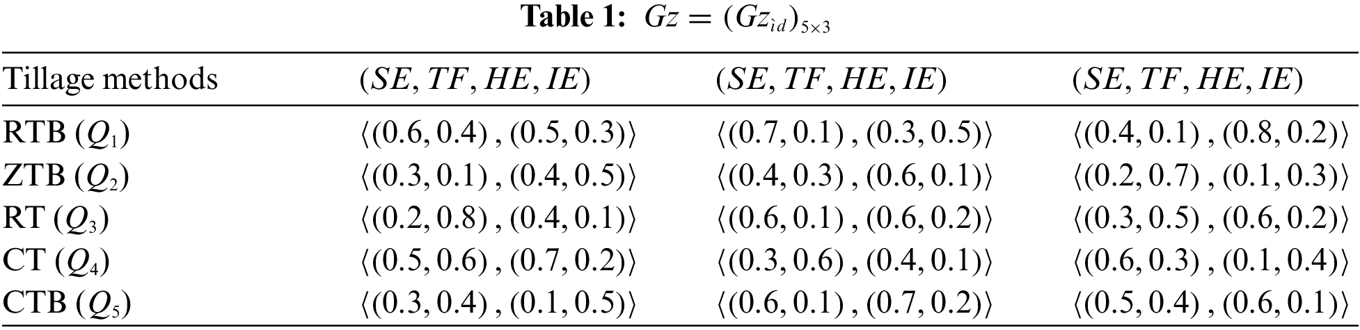
By using PFZNEWA operator: Now, we can apply PFZNEWA on Table 1.
Step 1: To find PFZNs
The calculation step for Table 1 PFZNEWA operator for the first step
i.e.,
Thus
Step 2: The score values
Step 3: According to the score values
Here we first order the given matrix with the help of score function then the original matrix becomes: By using PFZNEOWA operator: Now, we can apply PFZNEOWA on Table 1.
Step 1: To find
Step 2: The score values
Step 3: According to the score values
By using PFZNEWGA operator: Now, we can apply PFZNEWGA on Table 1.
Step 1: The total number of
Step 2: The score values
Step 3: According to the score values
Step 1: The total number of
Step 2: The score values
Step 3: According to the score values
8 Improved EDAS Method Based on Pythagorean Fuzzy Z-Number Einstein Aggregation Operators
MCDM is beneficial in locating solutions to a wide range of decision-making challenges that arise in the real world. Evaluation based on the distance from the average solution (EDAS) is an innovative and viable tool for MCDM tactic. The needed concerns, such as the average response being determined using weighted mean in this manner, may be effectively addressed by the EDAS technique. For the purpose of assessing the efficacy of the PFZN weighted geometric AOs, an original extended EDAS strategy is created to handle the complicated uncertain data in real-world DS scenarios. Assume there are a number of “alternatives”
Step 1: Select a set of qualities that can be used to evaluate the problem: Prospective assessment characteristics are acquired by a review of the literature, and an expert decision-making committee is established to filter the characteristics for the purpose to generate a legitimate set of evaluation criteria.
Step 2: Using normalization, the following steps are taken to construct the normalized decision matrix:
if
Step 3: Aggregated Data: The skilled uncertain data of required situations are aggregated using established PFZNWGA operators.
Step 4: Verify the average solution (
Step 5: The positive
The score function of
where W shows the score value.
Step 6: Calculate SPDA and SNDA, which represent for PDA and
Step 7: Normalize weighted sum of PDA and NDA is defined as, respectively
Step 8: Compute the values of ASC depends on each alternative’s as
Step 9: Depending on the ASC calculations, alternatives are sorted in decreasing order, and the higher the ASC number, the better options will be.
The flow chart of EDAS method is given in Fig. 1.
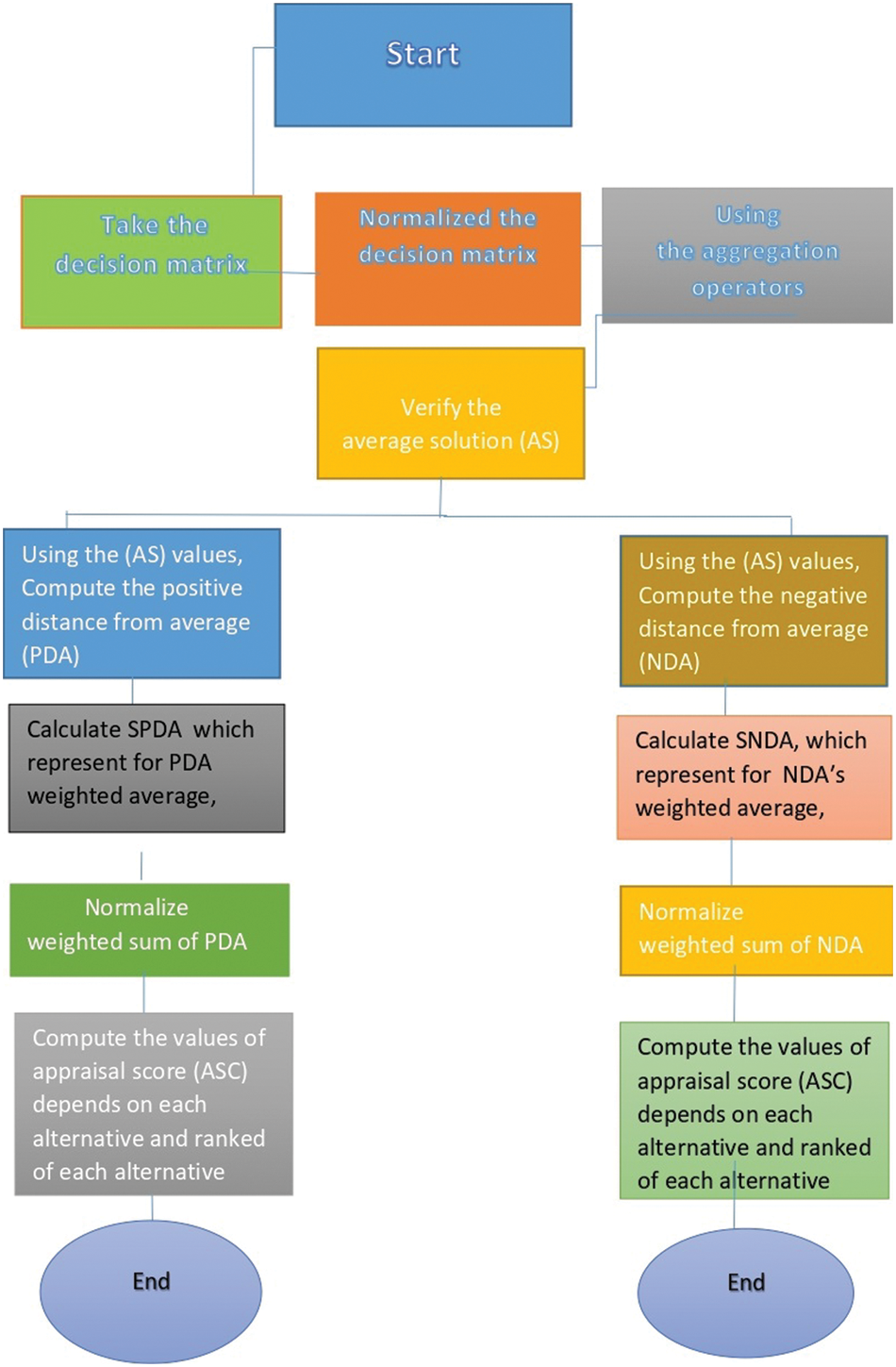
Figure 1: Flow chart of EDAS method
8.1 Numerical Illustration by Using EDAS Method
Step 1: The expert decision information is given in Table 2.
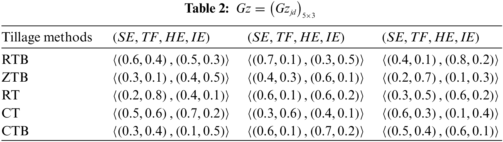
Step 2: The normalized decision matrix is created using normalization as follows:
if
Step 4: The score values
And verify the average solution (
Score function of average solution (
Step 5: Using the
By using the score function of
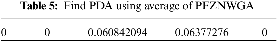
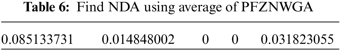
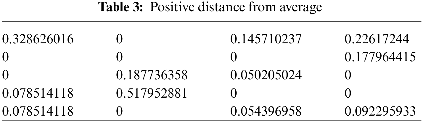
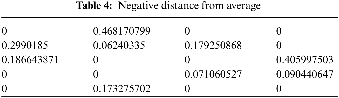
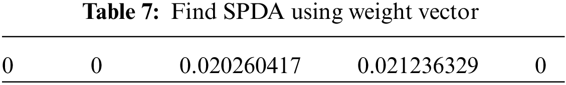
Step 6: Determined SPDA and SNDA in Tables 7 and 8, respectively, which reflect the weighted average for PDA and
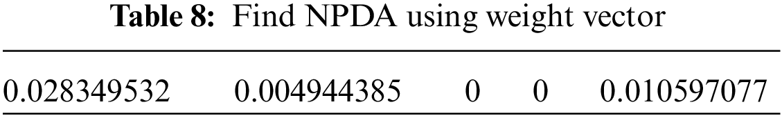
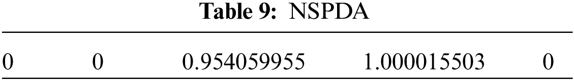
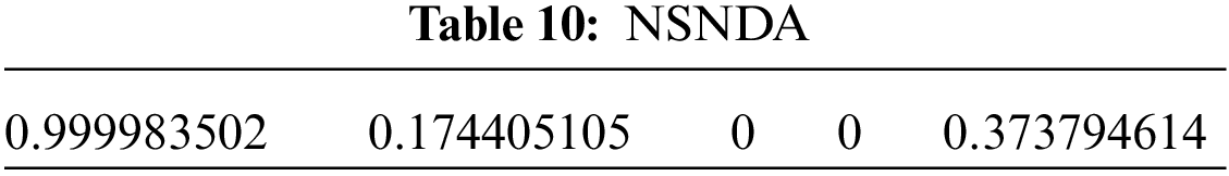
Step 7: The total PDA and NDA is presented in Tables 9 and 10, respectively, normalized by weight are characterized as:
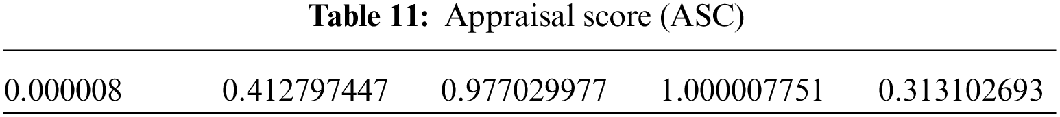
Step 8: Values of the ASC are determined in Table 11:
Step 9: Ranking of EDAS method is given in Table 12 by using weighted geometric aggregation operator:

Validation and Sensitivity Analysis
This section provides an example concerning the challenges that are faced in the agricultural fields, such as the productivity, profitability, and energy use efficiency of wheat crops grown under a variety of tillage systems. The purpose of this section is to illustrate the relevance and efficacy of the developed MCDM technique with PFZN information. Energy input estimates were based on the amount of human labor needed, the use of various kinds of equipment, and the amount of materials. Energy calculations were carried out using various input and output energy equivalents. Since the price of fuel continues to rise, there is a growing interest in improving agricultural production’s energy efficiency. To meet the needs of a more populous world, other industries, like agriculture, had to rely on non-renewable energy sources like electricity and fossil fuels to manufacture more food than was required.
Here, sensitivity analysis is performed to adjust the behavior of the offered methodologies. In Table 2, we provide five sets of possibilities. One criterion has a higher weight than the others for each set, as shown in the table. By following this technique, a large enough space of criterion weights has been constructed to test the method’s sensitivity to changes in the weighting of criteria. In Table 13 and Fig. 2, we provide the results of a sensitivity study that ranks different operators based on an extended EDAS method amenity alternative and a variety of criterion weight.
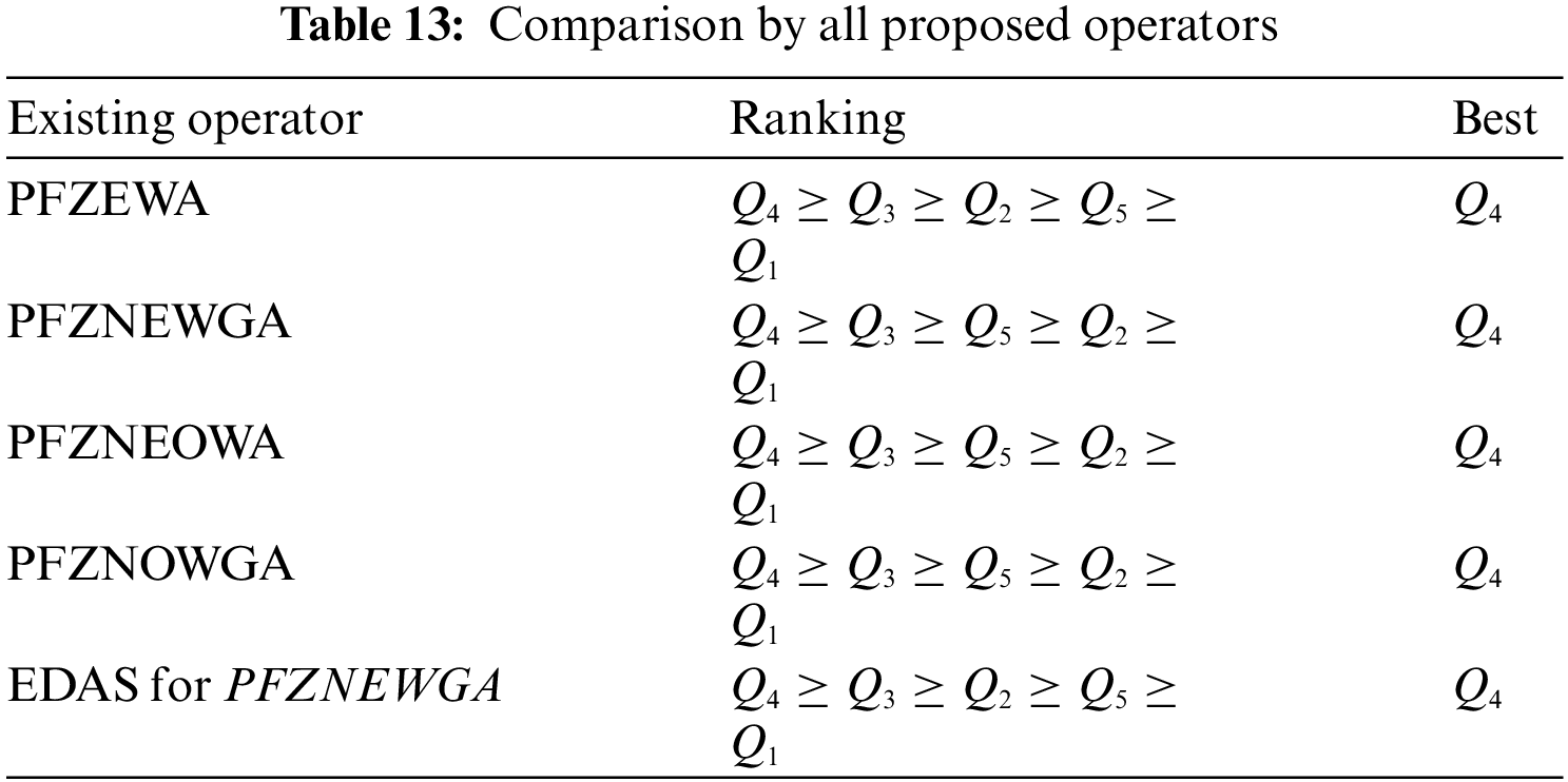
Figure 2: Ranking results
The graphical representation of ranking result is shown with the help of a Fig. 2.
In this section we discussed the ranking results with the existing studies in the literature. The Tables 14 and 15 are given as follows:
The wheat crop had a distinct set of energy inputs compared to the other crops. The primary reason for the disparity in wheat energy inputs was the use of different fuels. There is a need for human labor, irrigation, and seed energy. Different types of tillage required different types of energy expenditure, one of which was higher in CTB. CT, RTB, RT, and ZTB all help to reduce fuel energy use when applied to wheat crops. The performance values of alternatives in MCDM circumstances are prone to being distributed arbitrarily, despite the fact that these values are essential in a wide variety of scientific, technical, and managerial disciplines. The optimistic assessment score and the pessimistic assessment score were used together to make the enhanced evaluation score, which was then used to make the final evaluation of the different options. We have defined favorable and unfavorable values for a number of components of the recommended method in order to account for the unpredictability of the data across the entire analytic strategy. This is done to work through numerical examples and demonstrate how the proposed method functions, as well as showcase the situations where it may be useful. We use the second example to compare the ranking results of the recommended technique with a few other ways, and the first example gives a step-by-step discussion of the EDAS strategy. In addition, the decisive rating outcomes of the competitions that were recommended were better aligned with the real decision-making techniques that were used.
Future Scope and Direction
There are several future research directions that can be explored based on the proposed method of handling Pythagorean fuzzy Z-numbers with Einstein aggregation operators and extended EDAS method. Some of these directions include:
1. Developing hybrid methods: The proposed method can be combined with other existing methods, such as TOPSIS, AHP, or PROMETHEE, to enhance its performance and accuracy.
2. Generalizing the proposed method: The proposed method can be generalized to handle other types of fuzzy numbers, such as interval-valued fuzzy numbers, type-2 fuzzy sets, and hesitant fuzzy sets.
3. Applications in diverse fields: The proposed method can be applied to various real-life problems, such as supplier selection, project evaluation, medical diagnosis, financial analysis, and environmental management.
4. Extending the EDAS method: The EDAS method can be further extended by incorporating additional distance metrics or modifying the weights calculation to improve its performance.
5. Development of software tools: Software tools can be developed to facilitate the implementation of the proposed method in decision-making problems.
6. The proposed method can be applicable to several real-life problems that involve decision-making under uncertainty and imprecision. For instance, in supplier selection, the proposed method can be used to evaluate and rank potential suppliers based on multiple criteria, such as quality, price, and delivery time. In financial analysis, the proposed method can be used to evaluate investment opportunities based on factors such as risk, return, and liquidity. In medical diagnosis, the proposed method can be used to analyze patient data and provide a diagnosis based on multiple symptoms and test results. Overall, the proposed method has the potential to be widely applied in various fields and can contribute to making more accurate and informed decisions in uncertain and imprecise situations.
Acknowledgement: The authors would like to thank the editors and the anonymous evaluators for their insightful and useful comments and suggestions, which significantly improved this article.
Funding Statement: The authors received no specific funding for this study.
Conflicts of Interest: The authors declare that they have no conflicts of interest to report regarding the present study.
References
1. Munde, A., Arora, H. D. (2022). A theoretical approach of information measure for pythagorean fuzzy sets. In: IOT with smart systems, pp. 1–7, Singapore: Springer. [Google Scholar]
2. Zeng, W. Y., Cui, H. S., Liu, Y. Q., Yin, Q., Xu, Z. S. (2022). Novel distance measure between intuitionistic fuzzy sets and its application in pattern recognition. Iranian Journal of Fuzzy Systems, 19(3), 127–137. [Google Scholar]
3. Sen, D. K., Datta, S., Mahapatra, S. S. (2018). Sustainable supplier selection in intuitionistic fuzzy environment: A decision-making perspective. Benchmarking: An International Journal, 25(2). [Google Scholar]
4. Rahman, K., Abdullah, S., Khan, M. A., Ibrar, M., Husain, F. (2017). Some basic operations on Pythagorean fuzzy sets. Journal of Applied Environmental and Biological Sciences, 7(1), 111–119. [Google Scholar]
5. Wei, G., Lu, M. (2018). Pythagorean fuzzy power aggregation operators in multiple attribute decision making. International Journal of Intelligent Systems, 33(1), 169–186. [Google Scholar]
6. Ejegwa, P. A. (2019). Pythagorean fuzzy set and its application in career placements based on academic performance using max–min–max composition. Complex & Intelligent Systems, 5(2), 165–175. [Google Scholar]
7. Keshavarz Ghorabaee, M., Amiri, M., Zavadskas, E. K., Turskis, Z., Antucheviciene, J. (2017). Stochastic EDAS method for multi-criteria decision-making with normally distributed data. Journal of Intelligent & Fuzzy Systems, 33(3), 1627–1638. [Google Scholar]
8. Oz, N. E., Mete, S., Serin, F., Gul, M. (2019). Risk assessment for clearing and grading process of a natural gas pipeline project: An extended TOPSIS model with Pythagorean fuzzy sets for prioritizing hazards. Human and Ecological Risk Assessment: An International Journal, 25(6), 1615–1632. [Google Scholar]
9. Yager, R. R., Abbasov, A. M. (2013). Pythagorean membership grades, complex numbers, and decision making. International Journal of Intelligent Systems, 28(5), 436–452. [Google Scholar]
10. Wang, J. Q., Cao, Y. X., Zhang, H. Y. (2017). Multi-criteria decision-making method based on distance measure and Choquet integral for linguistic Z-numbers. Cognitive Computation, 9(6), 827–842. [Google Scholar]
11. Tian, Y., Kang, B. (2020). A modified method of generating Z-number based on OWA weights and maximum entropy. Soft Computing, 24(20), 15841–15852. [Google Scholar]
12. Jia, Q., Hu, J., Herrera-Viedma, E. (2021). A novel solution for Z-numbers based on complex fuzzy sets and its application in decision-making system. IEEE Transactions on Fuzzy Systems, 30(10), 4102–4114. [Google Scholar]
13. Atanassov, K. (1986). Intuitionistic fuzzy sets. Fuzzy Sets and Systems, 20, 87–96. [Google Scholar]
14. Aliev, R. A., Pedrycz, W., Huseynov, O. H. (2018). Functions defined on a set of Z-numbers. Information Sciences, 423, 353–375. [Google Scholar]
15. Poleshchuk, O. M. (2019). Novel approach to multicriteria decision making under Z-information. 2019 International Russian Automation Conference (RusAutoCon), pp. 1–5. IEEE. [Google Scholar]
16. Jiang, W., Cao, Y., Deng, X. (2019). A novel Z-network model based on Bayesian network and Z-number. IEEE Transactions on Fuzzy Systems, 28(8), 1585–1599. [Google Scholar]
17. Kang, B., Zhang, P., Gao, Z., Chhipi-Shrestha, G., Hewage, K. et al. (2020). Environmental assessment under uncertainty using Dempster-Shafer theory and Z-numbers. Journal of Ambient Intelligence and Humanized Computing, 11, 2041–2060. [Google Scholar]
18. Jabbarova, A. I. (2017). Application of Z-number concept to supplier selection problem. Procedia Computer Science, 120, 473–477. [Google Scholar]
19. Abiyev, R. H., Günsel, I., Akkaya, N. (2020). Z-number based fuzzy system for control of omnidirectional robot. 10th International Conference on Theory and Application of Soft Computing, Computing with Words and Perceptions-ICSCCW-2019, pp. 470–478. Springer International Publishing. [Google Scholar]
20. Pal, S. K., Banerjee, R., Dutta, S., Sarma, S. S. (2013). An insight into the Z-number approach to CWW. Fundamenta Informaticae, 124(1–2), 197–229. [Google Scholar]
21. Ding, X. F., Zhu, L. X., Lu, M. S., Wang, Q., Feng, Y. Q. (2020). A novel linguistic Z-number QUALIFLEX method and its application to large group emergency decision making. Scientific Programming, 2020, 1631869. https://doi.org/10.1155/2020/1631869 [Google Scholar] [CrossRef]
22. Kang, B., Hu, Y., Deng, Y., Zhou, D. (2016). A new methodology of multicriteria decision-making in supplier selection based on-numbers. Mathematical Problems in Engineering, 2016, 8475987. https://doi.org/10.1155/2016/8475987 [Google Scholar] [CrossRef]
23. Ren, Z., Liao, H., Liu, Y. (2020). Generalized Z-numbers with hesitant fuzzy linguistic information and its application to medicine selection for the patients with mild symptoms of the COVID-19. Computers & Industrial Engineering, 145, 106517. [Google Scholar]
24. Garg, H. (2017). A new improved score function of an interval-valued Pythagorean fuzzy set based TOPSIS method. International Journal for Uncertainty Quantification, 7(5), 463–474.https://doi.org/10.1615/Int.J.UncertaintyQuantification.2017020197 [Google Scholar] [CrossRef]
25. Garg, H. (2016). A new generalized improved score function of interval-valued intuitionistic fuzzy sets and applications in expert systems. Applied Soft Computing, 38, 988–999. [Google Scholar]
26. Riaz, M., Naeem, K., Chinram, R., Iampan, A. (2021). Pythagorean-polar fuzzy weighted aggregation operators and algorithm for the investment strategic decision making. Journal of Mathematics, 2021, 6644994. https://doi.org/10.1155/2021/6644994 [Google Scholar] [CrossRef]
27. Garg, H. (2019). New logarithmic operational laws and their aggregation operators for Pythagorean fuzzy set and their applications. International Journal of Intelligent Systems, 34(1), 82–106. [Google Scholar]
28. Du, S., Ye, J., Yong, R., Zhang, F. (2021). Some aggregation operators of neutrosophic Z-numbers and their multicriteria decision making method. Complex & Intelligent Systems, 7(1), 429–438. [Google Scholar]
29. Chaurasiya, R., Jain, D. (2023). Hybrid MCDM method on pythagorean fuzzy set and its application. Decision Making: Applications in Management and Engineering, 6(1), 379–398. https://doi.org/10.31181/dmame0306102022c [Google Scholar] [CrossRef]
30. Ashraf, A., Ullah, K., Hussain, A., Bari, M. (2022). Interval-valued picture fuzzy Maclaurin symmetric mean operator with application in multiple attribute decision-making. Reports in Mechanical Engineering, 3(1), 210–226. [Google Scholar]
31. Sahu, R., Dash, S. R., Das, S. (2021). Career selection of students using hybridized distance measure based on picture fuzzy set and rough set theory. Decision Making: Applications in Management and Engineering, 4(1), 104–1263. [Google Scholar]
32. Yildirim, B. F., Yildirim, S. K. (2022). Evaluating the satisfaction level of citizens in municipality services by using picture fuzzy VIKOR method: 2014–2019 period analysis. Decision Making: Applications in Management and Engineering, 5(1), 50–66. [Google Scholar]
33. Ali, S., Kousar, M., Xin, Q., Pamucar, D., Hameed, M. S. et al. (2021). Belief and possibility belief interval-valued N-soft set and their applications in multi-attribute decision-making problems. Entropy, 23(11), 1498 [Google Scholar] [PubMed]
34. Hameed, M. S., Ahmad, Z., Ali, S., Mahu, A. L., Mosa, W. F. (2022). Multicriteria decision-making problem via weighted cosine similarity measure and several characterizations of hypergroup and (Weak) polygroups under the triplet single-valued neutrosophic structure. Mathematical Problems in Engineering, 2022, 1743296. https://doi.org/10.1155/2022/1743296 [Google Scholar] [CrossRef]
35. Deschrijver, G., Kerre, E. E. (2002). A generalization of operators on intuitionistic fuzzy sets using triangular norms and conorms. Notes on Intuitionistic Fuzzy Sets, 8(1), 19–27. [Google Scholar]
36. Zadeh, L. A. (1965). Fuzzy sets. Information and Control, 8(3), 338–353. [Google Scholar]
37. Zadeh, L. A. (2011). A note on Z-numbers. Information Sciences, 181(14), 2923–2932. [Google Scholar]
Cite This Article
 Copyright © 2023 The Author(s). Published by Tech Science Press.
This work is licensed under a Creative Commons Attribution 4.0 International License , which permits unrestricted use, distribution, and reproduction in any medium, provided the original work is properly cited.
 Downloads
 Citation Tools