Optimization of Engine Control Strategies for Low Fuel Consumption in Heavy-Duty Commercial Vehicles

1  Introduction

It is well-known that vehicle energy consumption and exhaust emissions harm sustainable development. The rapid growth of the automobile industry in developing countries has alarmingly exacerbated the environmental pollution caused by automobile exhaust emissions [1]. According to the literature, more than half of the energy used for trucking comes from heavy-duty commercial vehicles [2]. Therefore, there is an urgent need for the development of heavy-duty commercial vehicles to lower exhaust emissions in the transportation industry.

Although numerous methods for reducing vehicle fuel consumption have been proposed, they are influenced by several factors [3]. Eco-driving techniques including acceleration, cruising, deceleration, and stopping, as well as other elements including traffic, vehicles, and the environment, are regarded as low-cost and efficient strategies to increase fuel efficiency [4,5]. Compared to unpredictable driving, a smooth driving style can simultaneously reduce fuel consumption and increase driving comfort and safety. Moreover, drivers who practice eco-driving must minimize idling, excessive braking, acceleration, and other driving habits. 16 separate driving factors have been also studied for their impact on fuel consumption and emissions, four of which play an important role and are related to the acceleration and power requirements [6].

Fuel economy studies rely on specific scenarios and driving strategies that are more sensitive to speed and acceleration [7]. Acceleration and deceleration are considered important factors influencing fuel economy and exhaust emissions. As a result, finding the optimal speed trajectory or strategy has attracted wide attention from the scientific community. Choi et al. [8] concluded the key factors leading to the sudden increase in fuel consumption of LPG passenger vehicles. Chakraborty et al. [9] proposed a multi-dimensional heuristic system to effectively lower energy use while the vehicle is waiting. Birrell et al. [10] recommend smooth and positive acceleration for cruising speed, and limiting throttle opening to less than 50%. Although some contributions to vehicle eco-driving were achieved by the above-mentioned works, they were all limited to low-speed passenger vehicles.

Since the creation of eco-driving techniques for heavy-duty commercial vehicles is highly dependent on vehicle performance, road driving, and traffic environment availability, the relevant works in the literature are scarce. Although planning the optimal speed profile of a vehicle using a heavy vehicle driving model predictive control (MPC) [11,12] algorithm was initially believed that could minimize fuel consumption, the connection between environmental driving forces and fuel consumption, as well as the impact of heavy vehicle engine factors on fuel consumption, have not been investigated in the literature. On top of that, the experimental speed trajectory planning must satisfy the condition that the speed of the target vehicle is constant [13]. Even though an optimal path and speed trajectory planning strategy for heavy commercial vehicles to drive with low fuel consumption on urban roads has been proposed, the impact of fuel consumption estimation and vehicle dynamics models for heavy vehicles on ecological driving factors has not yet been taken into account.

Under this perspective, in this work, an engine control strategy for heavy commercial vehicles that use less fuel was proposed and optimized. The optimal driving strategy for heavy-duty commercial vehicles that minimizes fuel consumption can be classified as optimal control, with the optimization objective of minimizing fuel consumption during vehicle operation. The factors causing low fuel consumption driving of heavy-duty commercial vehicles were also thoroughly discussed, and a driving strategy based on speed profile and throttle opening was proposed. Three parameterization methods were used to optimize the engine control strategy. Interestingly, iterating with the global optimization algorithm yielded the best results. Finally, the effectiveness of the low-fuel consumption engine control strategy was demonstrated by comparing it to real-world vehicle test results.

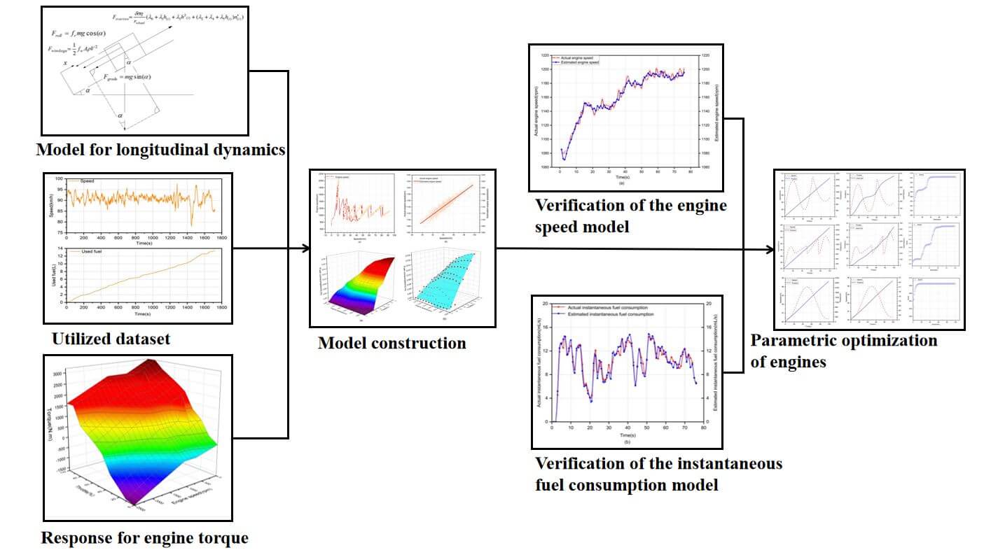
The remainder of this article is divided into the following sections: the discussion of a generic first-principles model of heavy-duty commercial vehicles in Section 2 and optimizes model parameters using real-world vehicle data. The parameterization and optimization algorithms for the optimal engine control problem are presented in Section 3. Section 4 compares the optimization outcomes of various heavy-duty commercial vehicle control strategies. Section 5 contains the conclusions of this paper.

2  Vehicle Dynamics Modeling

2.1 Model Derivation

The heavy-duty commercial vehicle model derivation was divided into two parts: the longitudinal motion control model derivation and the model derivation for fuel consumption estimation. Because the fuel consumption estimation model is heavily reliant on the vehicle motion control model, the vehicle motion control model was first established, and then a single-step solution for fuel consumption was realized. The fuel consumption optimization problem defined in Section 3 can be simplified to the greatest extent possible by decomposing the complex task of the entire vehicle eco-driving process.

The evaluation of vehicle motion control was described using fundamental physics laws and the basic parameters of the experimental vehicle. Because the purpose of this part was to develop a mathematical model of how a vehicle operates, simple polynomial functions and heavy vehicle parameters were used to approximate the vehicle dynamics model [14]. It has been demonstrated in the literature that the driving force of the vehicle is largely dependent on the throttle opening and the quadratic polynomial model based on the rolling characteristics. However, the driving force test for heavy vehicles is usually based on engine torque and power factors. Hence, the driving force of the vehicle was considered the engine torque ratio in this work, and the instantaneous torque is obtained from the instantaneous speed and throttle opening relationship equation.

To improve the model’s robustness and accuracy, the traditional power factor fuel consumption model contained more parameters and was more computationally intensive [15,16]. In this work, a lightweight fuel consumption model based on engine speed was also redesigned for heavy commercial vehicles to enhance the calculation and effectiveness evaluation of fuel use. The model of vehicle throttle opening, engine speed, and instantaneous fuel consumption laws was summarized by analyzing the basic laws, operating parameters, and actual working conditions of vehicles. In addition, the model was improved based on ecological driving factors, resulting in an instantaneous fuel consumption model that meets the operating laws of heavy vehicles.

2.1.1 Motion of Vehicle

In this work, the heavy-duty commercial vehicle was idealized as a mass point, with no regard for the shape or size of the vehicle. However, the aerodynamic effect is regarded as a critical factor in the vehicle model that affects vehicle movement, and the operating state of the vehicle, as well as specific parameters, such as the vehicle wind resistance coefficient, air density, and orthogonal projection area, must be considered.

Aerodynamic drag is determined by the wind drag coefficient fw, vehicle orthographic projection area A, and definition of aerodynamic pressure Q:

{Fwindage=fwAQQ=12ρV2(1)

where A denotes the projected area of the driving direction of the vehicle, ρ uses the typical air density at sea level, and V is the relative speed of the vehicle to the actual wind speed. fw represents the wind resistance coefficient to be determined. The driving conditions of commercial vehicles under the conditions of no wind were only considered here. Therefore, Fwindage was only proportional to the relative velocity V, and the relative speed V was vehicle speed x′.

Rolling resistance and slope resistance are defined by Froll and Fgrade, respectively, both of which are related to road slope α:

Froll=frmgcos⁡(α)(2)

Fgrade=mgsin⁡(α)(3)

where fr is the assessment of the rolling resistance ratio, and m refers to the overall mass of the heavy vehicle described in this work.

Ftraction=δσηrwheel(λ0+λ1h(t)+λ3h(t)2+(λ2+λ4+λ5h(t))n(t)′)(4)

where δ, σ represent transmission ratio and main transmission ratio, respectively, η stands for mechanical efficiency, rwheel signifies the radius of the tire, h(t) is the throttle opening, n(t)′ denotes the instantaneous engine speed, and λ0,λ1,λ2,λ3,λ4,λ5 are the undefined propulsive drag coefficients.

The forces on the heavy-duty commercial vehicle in the longitudinal dynamics model are depicted in Fig. 1. According to the second law of Newton, the longitudinal dynamic equation of a vehicle can be described as follows:

mx″=Ftraction−Fwindage−Froll−Fgrade(5)

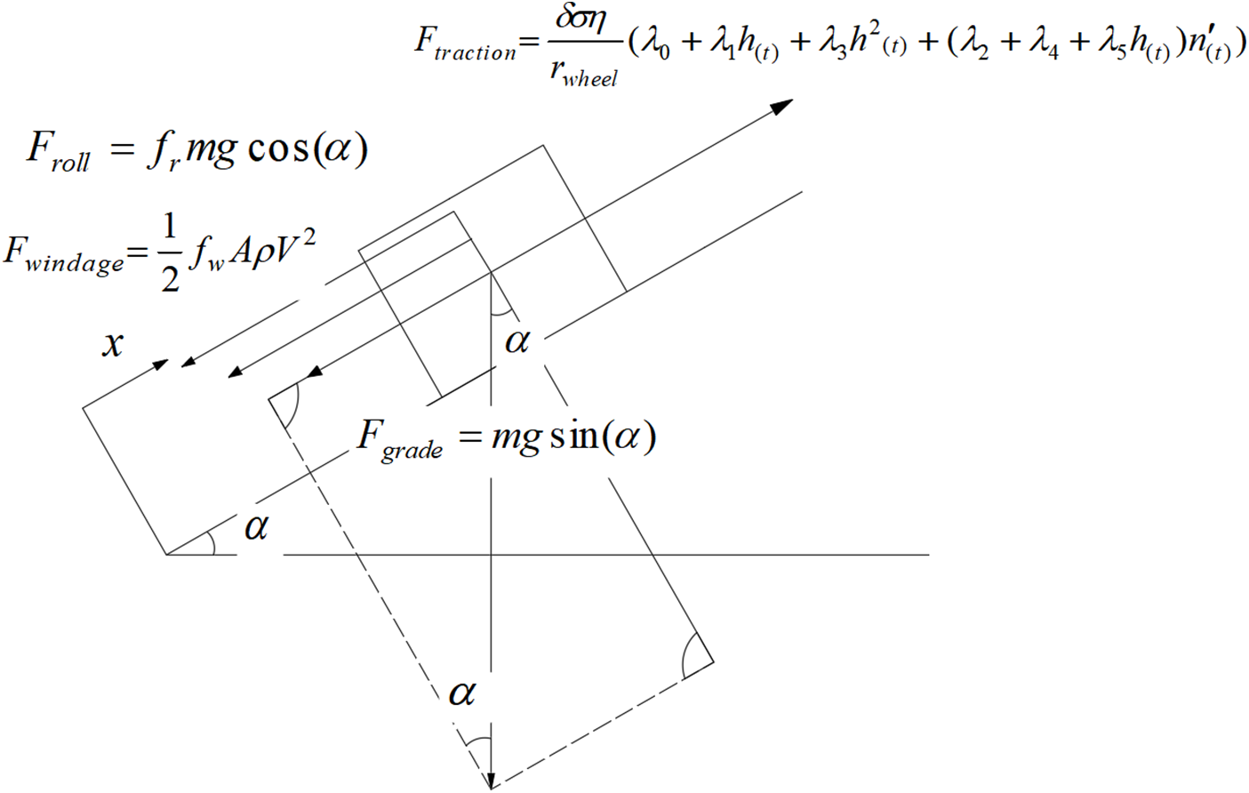
Figure 1: The forces on the heavy commercial vehicle in the longitudinal dynamics model

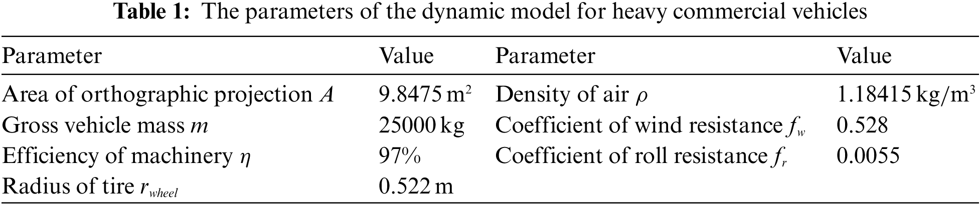
According to Eqs. (1)–(5), the dynamic balance Eq. (6) of heavy-duty commercial vehicles was obtained. The evaluation parameters of the heavy commercial vehicle dynamic model are presented in Table 1:

mx″=δσηrwheel(λ0+λ1h(t)+λ3h2(t)+(λ2+λ4+λ5h(t))n(t)′)−12fwAρx′2−frmgcos⁡(α)−mgsin⁡(α)(6)

2.1.2 Relationship between Fuel Consumption and Vehicle Speed

At present, there are two models available for fuel consumption estimation in the field of economic driving, and the pursuit of fuel consumption economy lies between them. The power demand type model typically calculates the instantaneous power demand of a vehicle and then obtains the instantaneous fuel consumption of the vehicle while driving using the speed and acceleration of heavy-duty commercial vehicles [17], as well as road and other information. On the other hand, the model of fuel consumption based on the universal characteristic curve is related to the characteristics and state of the engine, with better steady-state accuracy but poorer dynamic accuracy. The aforementioned factors lead to the implementation of a simplified fuel consumption model [18]. Instantaneous fuel efficiency is completely independent of fuel consumption in other periods. Additionally, the instantaneous fuel efficiency only serves as a gauge of the effectiveness of the control strategies. The precise cumulative fuel consumption value is unimportant in determining the performance of the different strategies relative to one another. As a result, the cumulative error brought on by model simplification needs not to be considered.

The instantaneous fuel injection rate of an engine is influenced by a variety of factors including engine throttle opening, coolant temperature, oxygen concentration at the intake valve position, engine speed, and torque [19]. Based on the connection between vehicle drive force (4), engine speed, and throttle opening, a model of instantaneous fuel consumption was developed based on engine speed and vehicle driving speed. Assuming full throttle opening, the fuel consumption estimation model is a function of engine speed and instantaneous fuel consumption rate. The pace at which fuel is consumed right now varies linearly with throttle opening when the speed is constant. As a result, the equation for estimating engine speed and fuel consumption rate was designed as Eq. (7).

Q(t)′=z0+ah(t)+bn(t)′+ch(t)2+dn(t)′+fh(t)n(t)′(7)

where n(t)′ is the instantaneous speed of the engine, h(t) denotes the relative opening of the throttle, the value range is 0% to 100%, z0,a,b,c,d,f are the adjustment parameters of the unknown fuel consumption estimation model, and Q(t)′ refers to the estimated instantaneous fuel consumption.

The vehicle speed, and acceleration for estimating the statistical function are considered the key factors for assessing fuel consumption. In addition, they are used to analyze the connection between engine speed and vehicle speed. When the vehicle speed is stable, the commercial vehicles have the same gear, speed, and the proposed linear change. The speed estimation model can be used to fit a primary function, whereas the instantaneous speed estimation model function is shown in Eq. (8).

n(t)′=r0x(t)′+r1(8)

where n(t)′ denotes the estimated rotational speed when the instantaneous speed of the vehicle is x(t)′, and r0,r1 are used to estimate the fitting parameters of the unknown speed model.

In summary, the direct relationship between the instantaneous fuel injection rate of the vehicle and the engine interior was considered first, and the fuel estimation model was established using engine speed and throttle opening, followed by an analysis of the relationship between the vehicle speed and acceleration and the engine interior. Finally, using Eqs. (7) and (8), the commercial vehicle driving instantaneous fuel consumption estimation model can be derived, as indicated in Eq. (9).

Q(t)′=ch(t)2+ah(t)+z0+[b+d+fh(t)][r0x(t)′+r1](9)

2.2 Tuning of Model Parameters

The employed parameter optimization was based on real-world data collected from heavy commercial vehicle experiments. During the experiments, the road surface is flat, and the changes caused by road inclination during vehicle driving can be ignored. Because the designed control system does not include the position factor of the vehicle, the data set does not contain vehicle position data. Fig. 2 depicts the data set used for parameter identification. A global positioning system (GPS) receiver determined the current speed, and a special gasoline flow meter measured the fuel consumption.

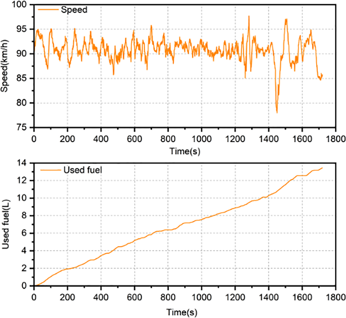
Figure 2: The dataset for identifying model parameters

Depending on engine experimental data, the parameters of the fuel consumption model were updated. For vehicle engines shifting from 700 to 1900 rpm and throttle position changing from 0% to 100%, the vehicle instantaneous fuel injection rate dataset was gathered in the engine tests, and the changing pattern of the pace of vehicle fuel consumption as engine speed grew when the throttle opening was taken from 0%–100%, respectively, is displayed in Fig. 3a.

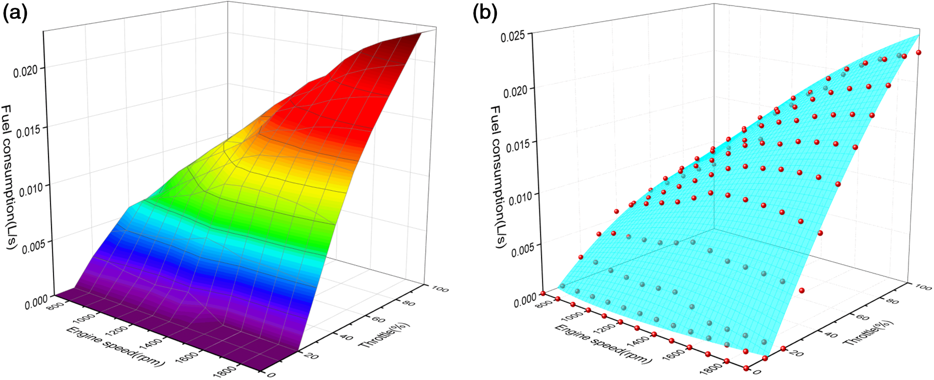
Figure 3: (a) The dataset for instantaneous fuel consumption; and (b) the estimation model of instantaneous fuel consumption

The instantaneous fuel consumption model is provided by Eq. (7). The conventional, linear model with linearly independent basis functions cannot be used because the experimentally derived data set was nonlinear. Because the proposed fuel consumption model has a two-dimensional input type in this work, the model parameters were identified using a nonlinear matrix fit. The sum of squared residuals (RSS) and the square of R (COD) were used as measurement bases to obtain more accurate model parameters [20].

RSS=∑i=1n⁡[yi−y∧]2(10)

COD=1−RSSTSS(11)

where yi denotes the observed value of the model, y∧ represents the estimated value of the model, TSS is the total sum of squares, and RSS refers to the statistical data obtained from general linear model analysis (such as traditional regression and variance analysis) [21]. Particularly, it represents the percentage of variance in the outcome variable (COD) and sample-wide estimate (the adjusted COD) that can be described by the predictor variable. The RSS determines the model parameter correlation, which generally measures the fitted expressions with fewer model parameters, while the residual sum of squares indicates the model error, whose error value is decreased with an increase in the fitting accuracy and is more accurate for the estimation of multi-parameter models [22]. Based on the fitting of the law between instantaneous fuel consumption, engine speed, and throttle opening, the obtained fuel consumption estimation model adjustment parameters are presented in Table 2.

The data shown in Table 2 are input to the instantaneous fuel consumption estimation model Eq. (7) for validation, and the final validation results were obtained in Fig. 3b. The static accuracy is higher in the given initial model. In the subsequent study, the fuel consumption estimation is performed for the vehicle during driving, and the extreme cases during engine testing did not occur. Therefore, the described control model (22) constrains the engine speed to 700–1400 rpm to further improve the accuracy of the model.

The given instantaneous fuel consumption estimation model can measure variables related to the engine, which cannot directly respond to the influence of speed factors on heavy vehicle fuel consumption. As a result, the following step was to examine the direct relationship between engine speed and vehicle speed. Fig. 4 depicts the experimental dataset for heavy commercial vehicle speed. When shifting gears, the engine speed of the vehicle changed with the gear. The primary function between the vehicle and engine speeds can be used as the functional relationship of the engine speed estimation model between the same gear, and the fitting adjustment parameters are presented in Table 3. The fuel consumption model for heavy-duty commercial vehicles developed in this work exhibited an RSS value of 1.11347×10−4 and a COD value of 0.962, which indicates a high degree of fitting accuracy.

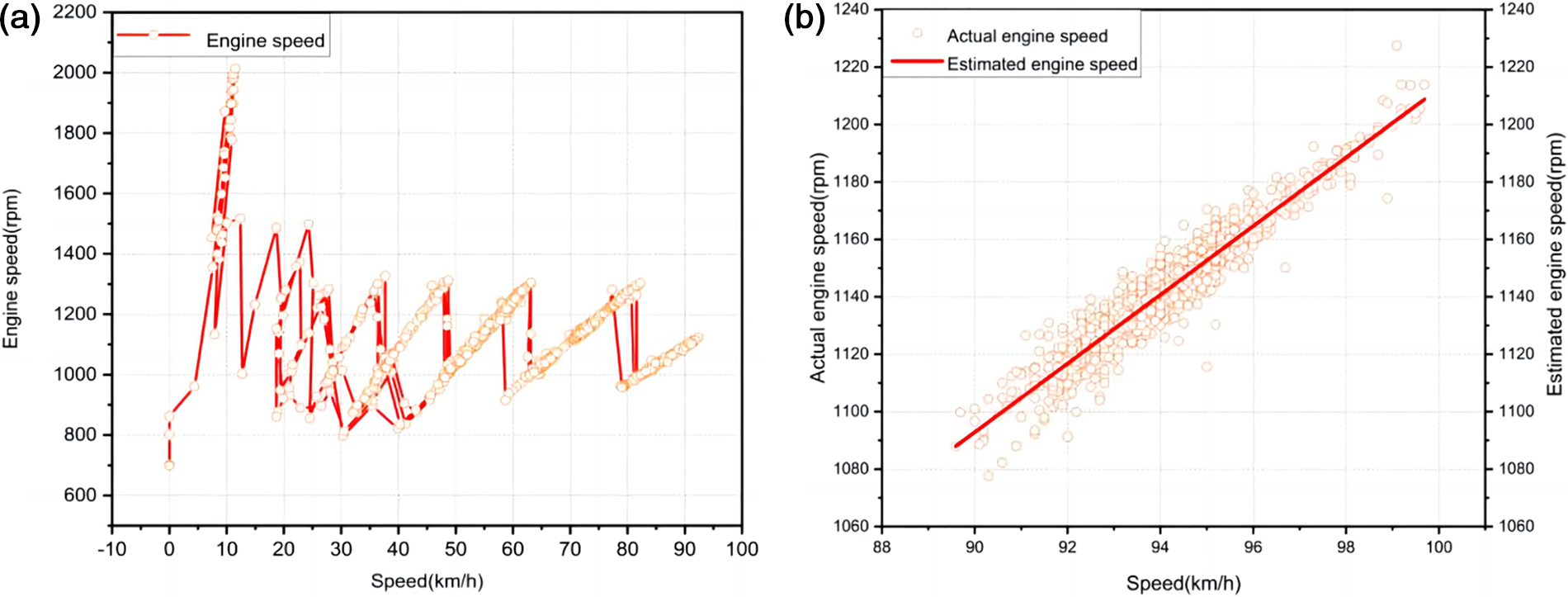
Figure 4: (a) The dataset for engine speed, and (b) the fitting of engine speed

The driveline transmits the torque produced by the car engine to the drive wheels, and the torque acting on the drive wheels creates a circular force on the ground, which is what propels the vehicle forward. As can be observed in Eq. (4), the driving force is proportional to the engine torque. The operating conditions of the engine are unstable while the vehicle is moving. Because there is a difference between the internal state of the engine and the external characteristics test when the throttle opening increased rapidly, the power that the engine can provide was slightly lower than when it was stable. The origins of this effect are that there is a difference between the internal state of the engine and the external characteristics test when the power performance was estimated. As a result, the relationship between torque and speed in the external characteristics curve under steady-state conditions was used for transmission system matching and optimization. The experiments in this work were specifically designed for engine torque, speed, and throttle opening. Fig. 5 displays the experimental data changing trend. The required engine driving resistance coefficient for heavy commercial vehicles can be calculated by analyzing the influence of engine speed on torque, as presented in Table 4.

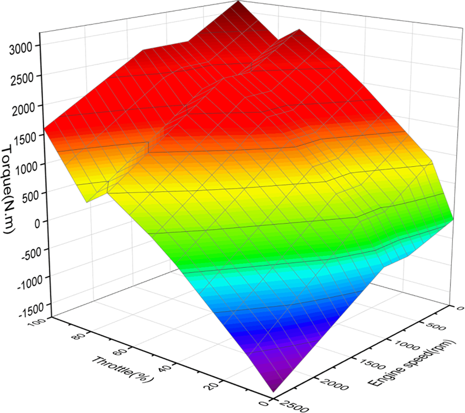
Figure 5: The dataset for torque

2.3 Verification of Models

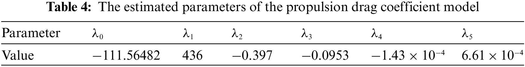
The verification of the model was based on an independent dataset obtained during the highway testing of the mentioned heavy trucks. The test conditions on this stretch of road were significantly different from the data used in the previous section. Fig. 6 depicts the collected experimental vehicle speed, fuel consumption, and time series [23]. The following is the basic flow of the model validation.

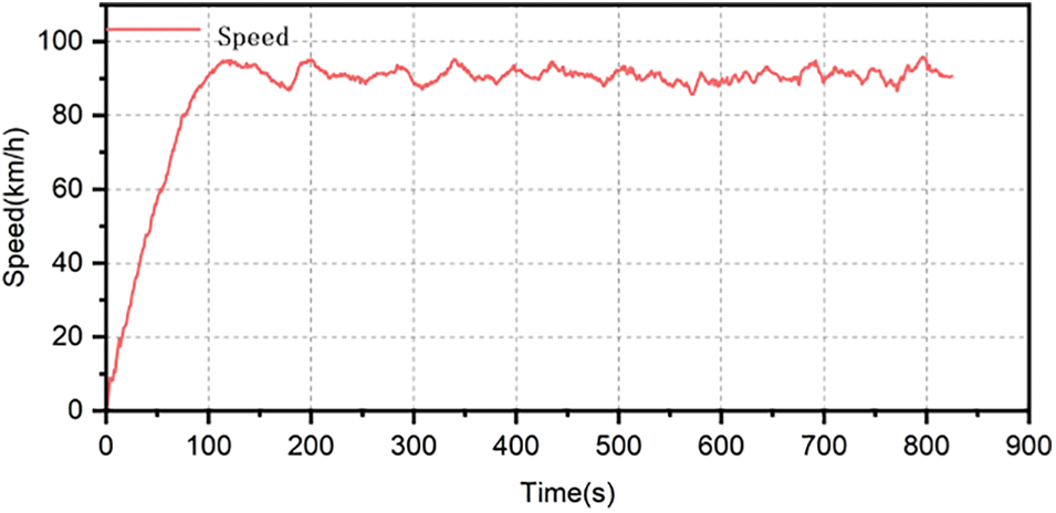
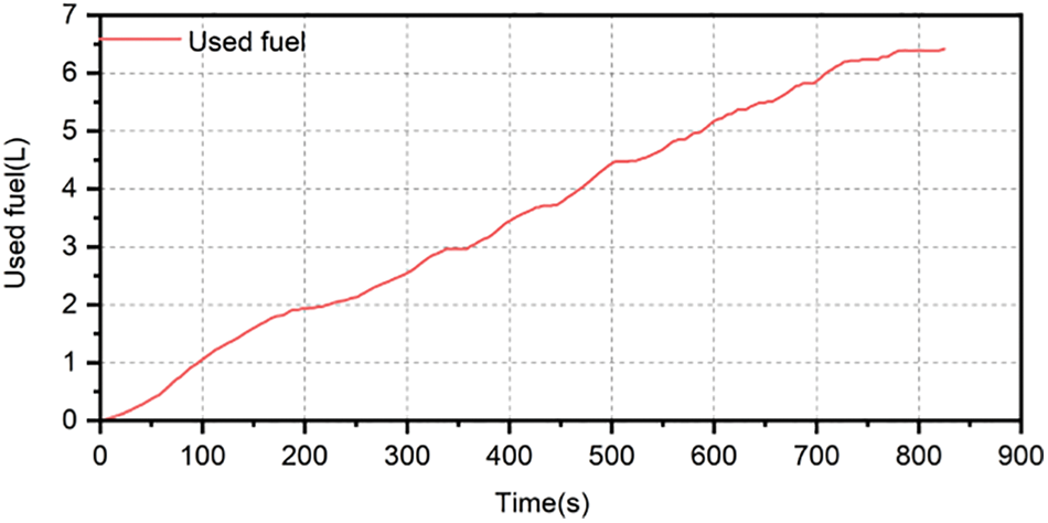
Figure 6: The dataset for validation of models

The relevant data snippet was selected from the dataset under test. Furthermore, the vehicle speed and fuel consumption data from the relevant time segment were used as the comparison condition because the fuel consumption of engines fluctuates with operating time. The vehicle speed was entered, the fuel consumption model simulation was run, and comparisons between the simulation and real-world results were performed. The model of the engine speed estimation was validated first. Fig. 7a illustrates a comparison of the model response speed to the actual speed. The simulation based on the model of engine speed estimation produced a relatively accurate result. When the actual speed oscillated more dramatically, the model can keep up in time to obtain accurate estimates, demonstrating a strong dynamic estimation performance.

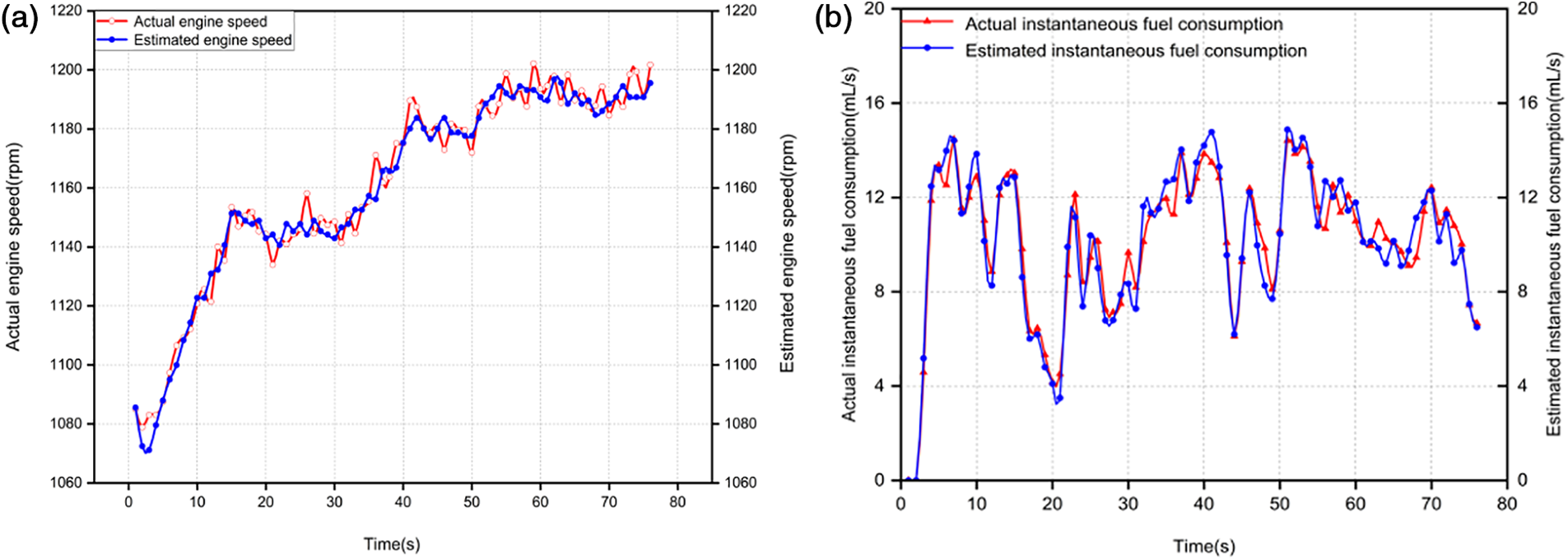
Figure 7: (a) The response of the engine speed model; (b) the response of the fuel consumption model

Following that, the model of fuel consumption estimation was validated. The desired speed, corresponding throttle opening, and total fuel consumption data were chosen from the dataset shown in Fig. 6, and the intercepted speed of the dataset was fed into the speed estimation model to obtain the speed required by the model of fuel consumption estimation. The estimated fuel consumption was calculated using the model of fuel consumption estimation and contrasted with the initial calculated fuel use, as displayed in Fig. 7b. The precise model can be used as the measurement basis for the subsequent control strategy, and the estimated trajectory of the tested model was close to the actual data trajectory. The mean relative error (MRE), a comparison of the anticipated, and actual values, were also used to assess the accuracy of the instantaneous fuel consumption model for predicting fuel consumption. The instantaneous fuel consumption model presented in this work had an MRE value of 0.08 and a relative error that can typically be controlled within 7%, which can satisfy the requirements of the following method. Since the model was tested using only the same initial conditions, the error between the model and the measured values was inevitable during the validation process. To obtain a more accurate model, more scenarios of validation data were needed. Thereby, the optimization of the model will be further enhanced in our future work.

3  Optimization of Engine Control Strategy for Heavy-Duty Commercial Vehicle

3.1 Establishment of an Optimization Problem

The strategy of creating a decision system based on objective laws, such as vehicle displacement, engine performance, fuel consumption, and other factors is appropriate given the existence of the longitudinal dynamics model of heavy commercial vehicles. The approach can compare many variables and reflect all that is available. The constraint of ordinary differential equations (ODE) formed by the vehicle motion equation, the engine speed model, and the fuel consumption estimation model are shown in Eqs. (12)–(15).

x1′=x2(12)

x2′=δσηmrwheel(λ0+λ1h(t)+λ3h2(t)+(λ2+λ4+λ5h(t))(r1+r0x2))−12mfwAρx22−frgcos⁡(α(x1))−gsin⁡(α(x1))(13)

x3′=r0x2+r1(14)

x4′=ch(t)2+ah(t)+z0+[b+d+fh(t)](r0x2+r1)(15)

where x1 is the vehicle driving position, x2 refers to the vehicle driving speed, x3′ is the engine speed, and x4 denotes the instantaneous fuel consumption of the vehicle engine.

To summarize the optimal control problem, for a controlled system, the optimal amount of control was sought to minimize the performance index while satisfying the constraints. The goal of this work was to find the vehicle driving control trajectory with the least amount of fuel consumption. Hence, the control trajectory was defined as a function of the vehicle position, vehicle speed, engine speed, and total engine fuel consumption, where vehicle speed and throttle opening were the control variables. In the vehicle driving process, seeking the optimal control trajectory is a nonlinear optimization with constraints. To determine the best control trajectory while a vehicle is running, a restricted nonlinear optimization procedure was used. For a controlled system, if the constraints are satisfied, the first thing to look for is the control variable u(t)∈Rm, control variable should be found to minimize the performance index J, as shown in Eq. (16).

minJ=∫t=t0t=tmaxGfuel(x1(t),u(t),x3′(t),t)+Φ(x4′(t0),u(t0),x4′(tf),u(tf),t0,tf)(16)

where Gfuel is the instantaneous fuel consumption rate and acceleration x2′ denotes the control variable u, whereas displacement x1, instantaneous speed x3′, and instantaneous fuel consumption x4′ are the state variables. Eq. (16) represents the performance indicator for solving the engine control plan while using the least amount of fuel. As can be seen from the equation, the equation constituting the vehicle driving fuel consumption index is composed of the integral of the state variable in the whole time domain from t0 to tmax, the composite function relation index of the control variable, and the sum of the composite function relation index of the instantaneous fuel consumption at the terminal moment of t0, tmax.

The variables of state and control satisfy the following constraints:

x4′(t)=Gfuel(x1(t),u(t),x4′(t),t)(17)

ϕ(x(t0),t0,x(tf),tf)=0(18)

C(u(t),x(t),t)≤0(19)

{x1(t0)=0x2(t0)=85x3′(t0)=0x1(tmax)=d(20)

x2(t)≥0(21)

700≤x3′(t0≤t≤tmax)≤1400(22)

Δx2′(t)=||x2′(ta)−x2′(tb)||||ta−tb||≤φ(23)

The variables of state and control constraints were explained as follows:

a.   Eq. (17) represents the composite equation of instantaneous fuel consumption estimation, which consists of state variable displacement, instantaneous speed, and control variable speed.

b.   Eq. (18) represents the boundary constraints of the state variables, which contains displacement, velocity, and engine speed constraints on the terminal moments (20), which are different from the terminal moment constraints in Eq. (17).

c.   Eq. (19) represents the process constraints, which were used to constrain the state and control variables (21)–(23) employed during the optimization process.

d.   The maximum vehicle engine torque was 2500 N.m., which corresponds to a speed range of 1000–1400 rpm. As a result, the speed range should satisfy Eq. (22) throughout the driving process.

e.   The rate of change in the driving acceleration of a vehicle is directly proportional to its fuel consumption, and the magnitude of the rate of change influences both driving comfort and safety. As a result, any period during vehicle operation must satisfy Eq. (23).

3.2 Optimization Algorithm

The optimization of the controlled systems (17)–(23) has two very important problems:

a.   Parameterization

Typically, the dynamic programming method is used to numerically solve the optimal strategy problem using the Behrman equation [24,25]. The time continuity issue necessitates the analysis of an unlimited number of potential states, which requires a significant amount of computer work. Therefore, the time continuity problem is usually discretized. However, a reasonable discretization time step is not determined, leading to difficulties in finding exact solution results.

Therefore, in this work, a parametric approach was to solve the optimal policy problem [26,27]. The optimal control strategy of the analytic function cannot be obtained directly, and some specific parameterization methods must be introduced to convert the optimization task into the form of a distributed search solution. However, during the process of finding a distributed solution, the excessive spatial dimensionality of the parameterization method can lead to difficulties in searching for the optimal solution quickly. Thus, it is important to select the appropriate optimization technique, which will hasten the convergence of the parameterization method.

b.   Nonlinearity

Since the maximization fuel consumption problem is a nonconvex, multimodal nonlinear model, it is difficult to be constrained, leading to the possible unsolvability of this optimization problem. Therefore, the objective function was used as the cost function (17), and the global optimization algorithm was utilized to calculate the result.

The Particle Swarm Optimization algorithm (PSO) is regarded as one of the more prominent options, and it follows the same general algorithmic flow as the global optimization approach [28], Weed Optimization algorithm (IWO) [29], Firefly algorithm [30], and Grey Wolf Optimization algorithm (GWO) [31]. At the beginning of the algorithm, a predetermined number of random particles was produced, and the parameters to be optimized during the process were measured, in terms of their merit at each stage according to the objective function. The optimization process updates the coordinates of the random vector according to some specific strategies, and the iterations were repeated until the iteration conditions were satisfied.

In the optimization of optimal fuel consumption strategy, the PSO algorithm has obvious advantages compared with other algorithms. More importantly, the best results can be obtained in a limited time through the PSO [32]. The PSO algorithm has been improved many times in the literature [33]. For example, the heuristic algorithm of the PSO algorithm was used as the target optimization model, or improved particle swarm optimization based on simulated annealing. However, in this work, the original model of the PSO algorithm was used as the solution tool [34]. When seeking the optimal solution, the algorithm needs to constantly iterate the trajectory of its generation i in the parameter space, adjust the local optimal coordinate pi pointing to the global optimal solution g, and calculate the number of steps according to the established acceleration constants c1,c2. The random weighting of the acceleration constant velocity and the diagonal matrix r1 and r2 with uniform distribution of random numbers at [0, 1] determine that the trajectory generated by the algorithm is semi-random.

di(t)=di(t−1)+si(t)(24)

si(t)=si(t−1)+c1(pi−di(t−1))r1+c2(g−di(t−1))r2(25)

To stop the optimization, it is necessary to make the optimization function meet the iteration condition (26).

f(di(t))≥pi,f(di(t))≥gi(26)

4  Parametrization Methods

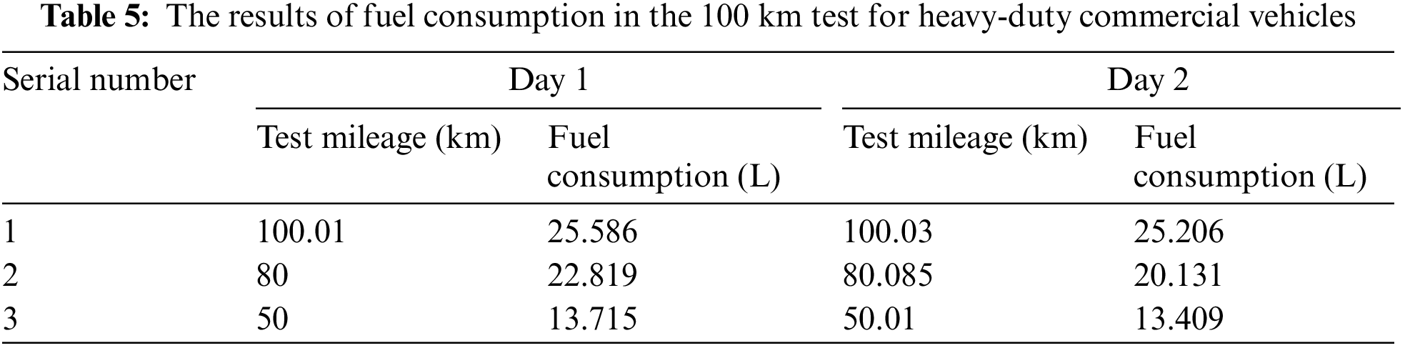
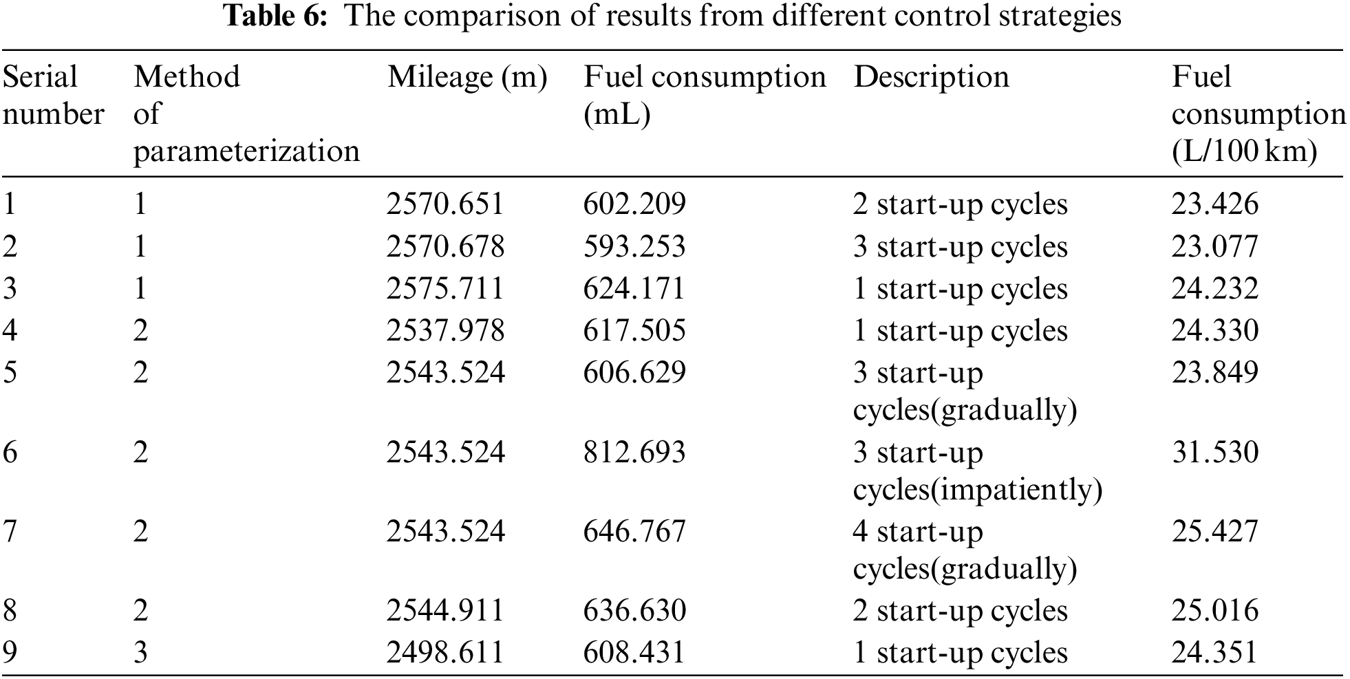
In Sections 4.1–4.3, the optimization outcomes of three distinct parameterization approaches for the control strategy were shown and reviewed. The results of the 100 km fuel consumption test in Table 5 and the different control strategies in Table 6 are compared in Section 4.4.

4.1 Parametrization Method 1: A Multi-Operation Strategy of Non-Variable Throttle Opening

In parametric approach 1, which models the regulating trajectory as the vehicle starting at a constant throttle opening, the throttle starts and stop moments were used as optimization parameters [35]. The existence of fewer parameters renders it easier for the algorithm to quickly resolve the issue because the strategy uses the global optimization approach and the breadth of the search space is determined by the number of variables that must be optimized [36]. By assuming that the decision dynamic array constraint value is the total number of parameters, and the start and stop moments of the throttle are used as the search space parameters, the search vector can be expressed by Eq. (27) as follows:

u=[s1,c1,s2,c2,…,sN,cN]T(27)

where sn is the nth start moment of throttle operation, cn denotes the nth stop moment of throttle operation, and N represents the number of throttle operations.

Since the throttle must be opened before it can be closed, the parameters in the decision vector must be strictly monotonically increased according to the time series. Moreover, the moment when the throttle was last closed must be lower than the maximum experimental time. For this reason, additional time constraints were imposed on the decision vector. Fig. 8 depicts the solution obtained by starting the PSO algorithm with a throttle opening twice, and Fig. 9 illustrates the convergence of the optimization process.

Figure 8: A solution obtained for non-variable throttle continuous operation 2 times strategy (parameterization method 2)

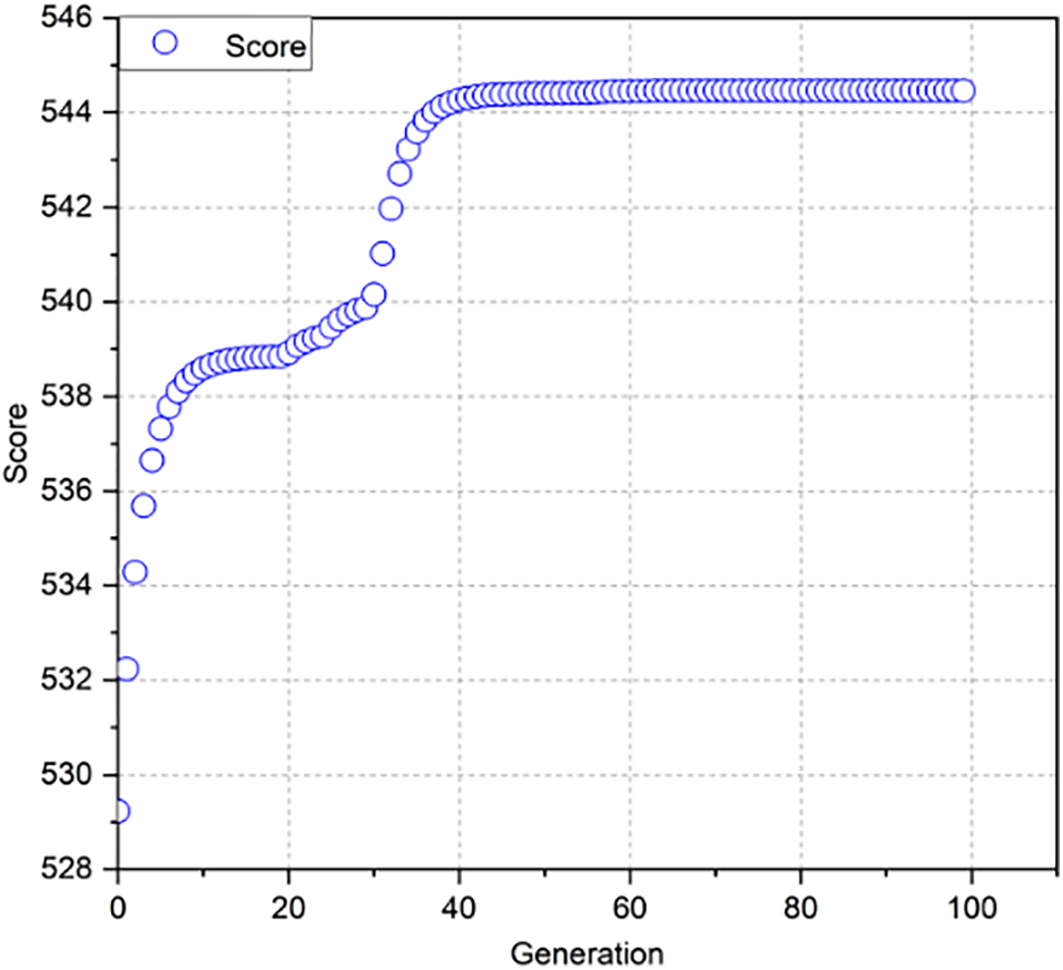
Figure 9: PSO algorithm progression to the non-variable throttling running condition 2 times strategy (parameterization method 2)

Experiments with 1 and 3 operation periods were also performed, achieving remarkably comparable state and control paths. Particularly, the primary distinction was defined as the number of starts raised, and the length of the throttle opening cycle shortened, leading to an increase in the frequency of vehicle speed changes. The fuel economy was not improved by increasing the number of parameters in the decision vector. Consequently, more iteration cycles were necessary for the algorithm to converge. As a result, as the vector dimension of the parameters increased, the algorithm converged more slowly. When method 1 with two start cycles of throttle opening was used, the convergence process required 40 iteration cycles. However, the convergence with three start cycles of throttle opening required 60 iteration cycles. This finding clearly indicates that the cost of algorithm convergence is increased with the number of parameters.

Heavy-duty commercial vehicles have a unique architecture, which makes air resistance and drive resistance important factors in evaluating fuel efficiency. The engine must have greater power to keep the car moving at a consistent speed. To avoid producing extra mechanical energy from rapid changes in vehicle speed, the running period of each cycle must be extended if more throttle-opening running cycles are necessary.

4.2 Parametrization Method 2: A Multi-Operation Strategy of Variable Throttle Opening

As a development of the control strategy covered in Section 4.1, the parameterization method with multiple throttle-opening start cycles and variable throttle-opening was proposed. Relative to the parameterization method 1, this strategy slightly increased the number of parameters in the optimization vector: the opening magnitude of the throttle opening during engine operation [37]. Thus, the search vector is shown in Eq. (28).

u=[s1,c1,r1,s2,c2,…,sN,cN,rN]T(28)

where sn is the nth start moment of throttle operation, cn refers to the nth stop moment of throttle operation, rn denotes the nth opening range of throttle operation, and N represents the number of throttle operations.

The maximum throttle opening constraint must be added to the constraints stated in parameterization method 1. The maximum throttle opening of 100% for heavy commercial vehicles provided by the experiment was specified. The periods of four consecutive throttle opening actions and the variable throttle opening for each period are displayed in Fig. 10. The relationship of the proposed control strategy to the non-variable throttle opening is shown in Fig. 8. However, in method 2, the throttle opening of the suggested method was changeable because each consecutive throttle operation was raised in comparison to the preceding one. It was conceivable that the driver achieved optimal fuel efficiency using various techniques for depressing the accelerator pedal in each of the other four approaches, as indicated in Table 6, which each involves accelerating with a different number of throttle operations for the same period.

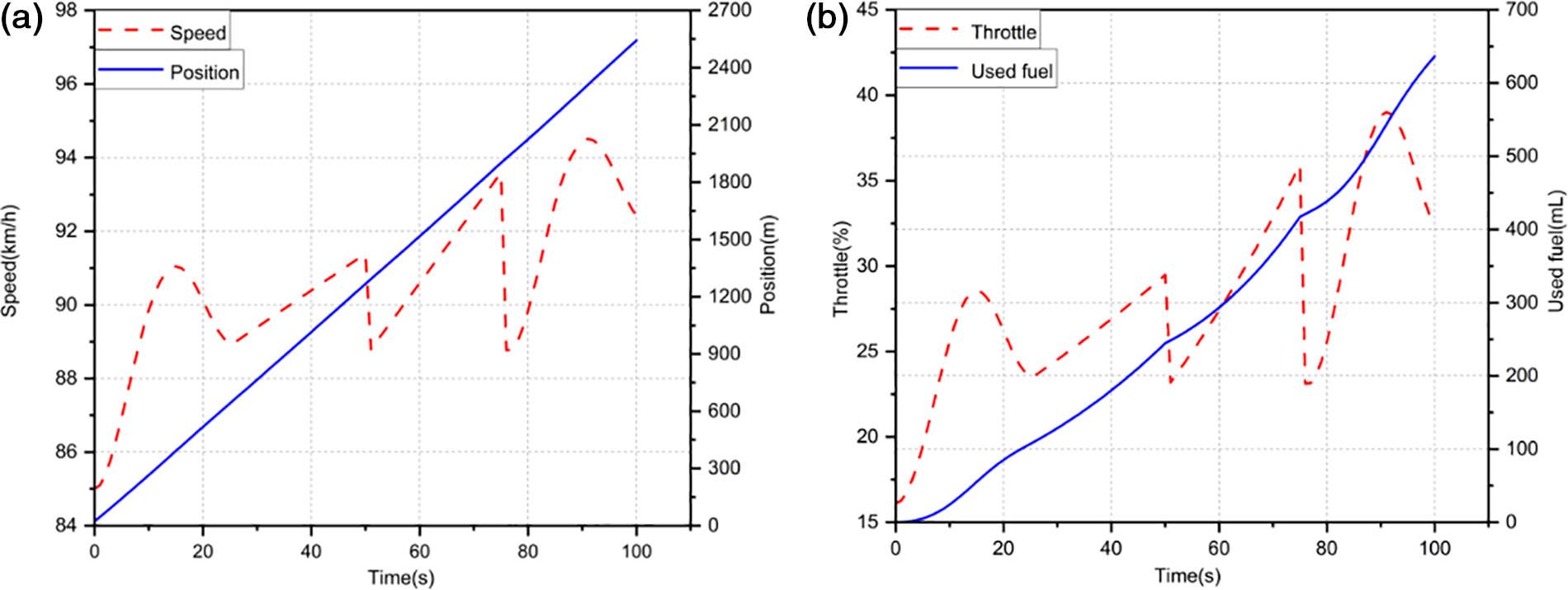
Figure 10: A solution obtained for variable throttle continuous operation 4 times strategy (parameterization method 2)

Different levels of throttle operation can also have a significant impact on the fuel consumption of heavy-duty commercial vehicles. Aggressive throttle pressing results in much higher fuel usage than progressive throttle pressing for the same number of throttle operations, as indicated by the comparison of data sets 5 and 6 in Table 6.

The convergence of the PSO algorithm to a variable throttle opening is illustrated in Fig. 11. As can be observed, with a variable throttle opening, the global optimization yields a cost 20 iterations higher than method 1 when the search vector is increased by the throttle opening magnitude. There is no significant difference in fuel consumption when the throttle opening magnitude is variable vs. non-variable. Nonetheless, the optimization technique becomes more difficult [38]. Therefore, the parameterized method with variable throttle opening is theoretically a more efficient strategy. The optimal fuel efficiency results cannot be obtained because imposing variable throttle opening parameters in the search vector leads to a reduced convergence rate. Therefore, it is difficult to guarantee a search for a definite local minimum in the search space.

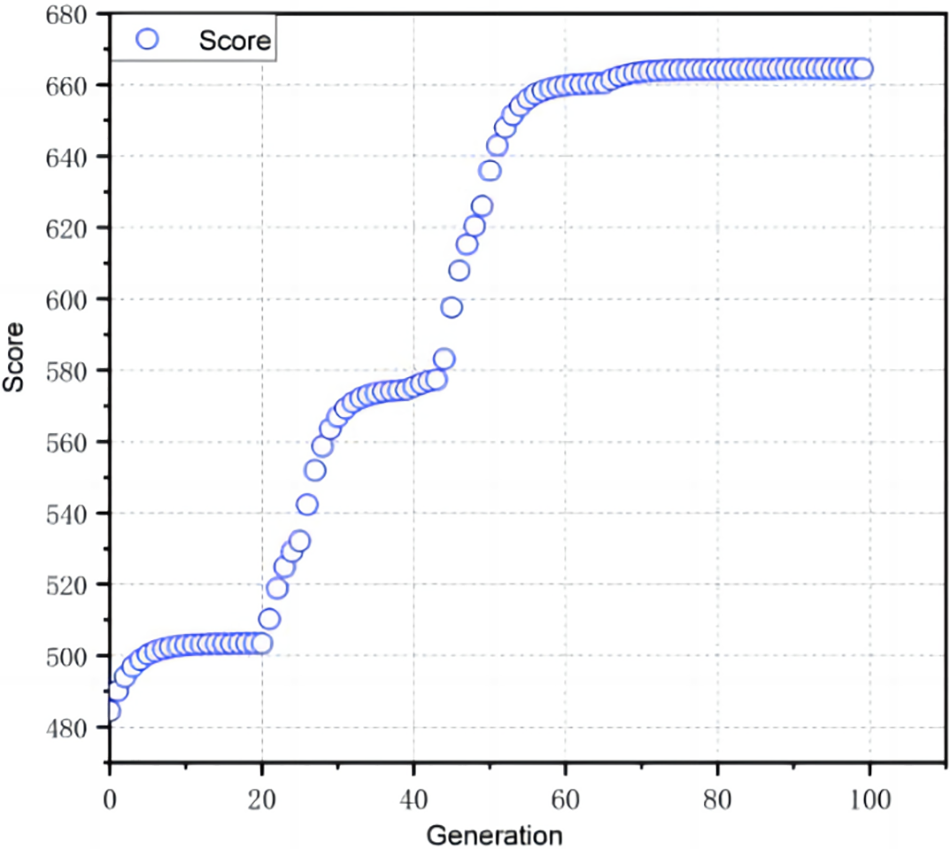
Figure 11: PSO algorithm progression to the variable throttle continuous operation 4 times strategy (parameterization method 2)

4.3 Parametrization Methods: A Single-Operation Strategy of Variable Throttle Opening

The third parameterization method operated with a single variable throttle from the start and runs until the end of the experiment. This control method was different from the one described in the preceding section in that it calls for only one actuation of the throttle opening. In addition, during the driving of the experimental vehicle, the mechanical energy generated by the engine was always higher than the energy necessary to drive the vehicle [39]. Therefore, in addition to constraining the throttle operation start and stop moments, the proposed parameterization method needed to assume that the throttle operation covered the maximum driving time, dividing this period into N periods, and constituting a decision variable with the throttle start and stop moments. The employed search vector is shown in Eq. (29).

u=[s1,c1,s1,s2,…,sN]T(29)

where sn is the nth start moment of throttle operation, cn refers to the nth stop moment of throttle operation, sn is the nth opening span of throttle operation, and N denotes the number of throttle operations.

Fig. 12 displays the single-start outcomes for the varied throttle openings. The progression of the PSO algorithm to a single operation strategy of variable throttle opening is illustrated in Fig. 13. The control trajectory of the optimal strategy is smooth and accelerates. It is safe to suppose that this method can best converge on a result that is like cycle control. The whole stroke cannot satisfy the running time of the full-time span strategy requirement. In contrast, a discretization approach to the periodic control strategy can also precisely determine the best control solution. Nonetheless, because of the complexity of the process and the high number of optimization factors, it is more expensive to solve.

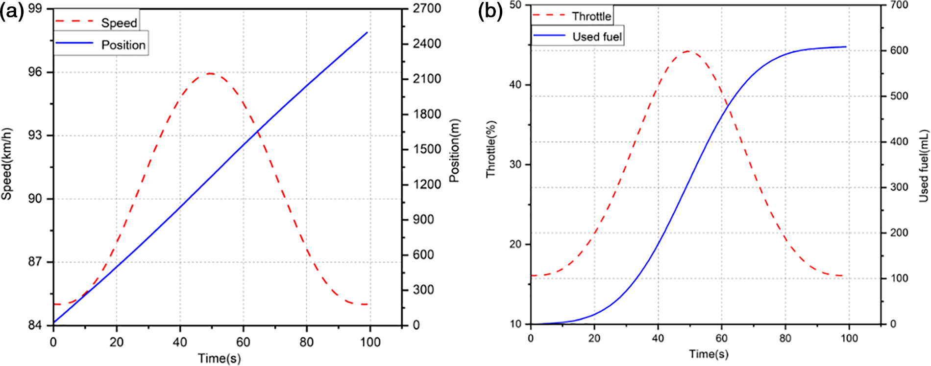
Figure 12: A solution obtained for a single operation strategy of variable throttle opening (parameterization method 3)

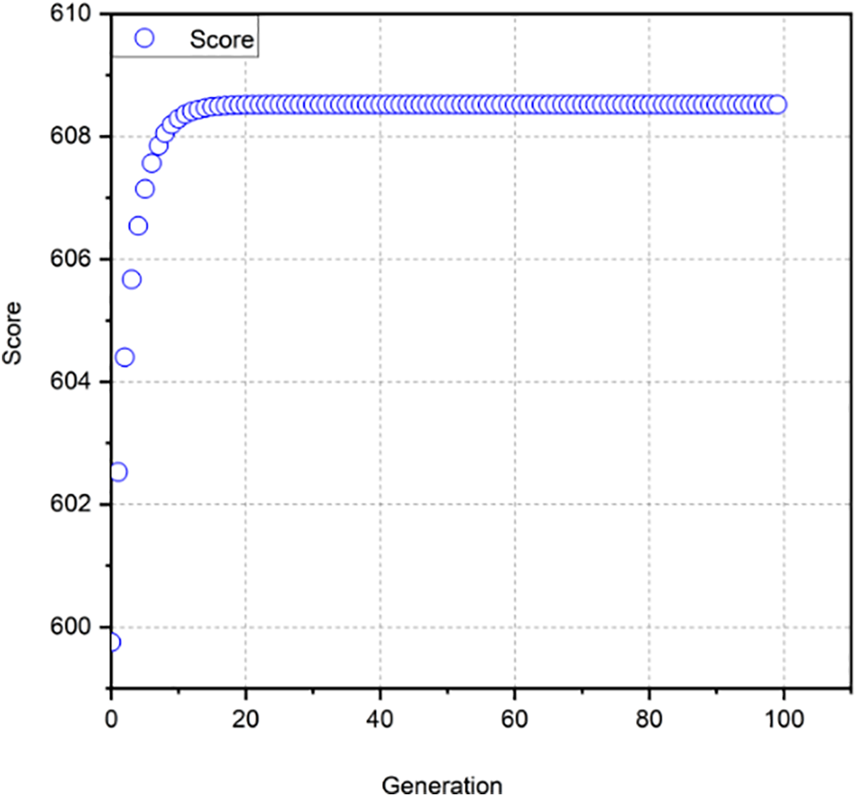
Figure 13: PSO algorithm progression to single operation strategy of variable throttle opening (parameterization method 3)

4.4 Experimental Results

Tables 5 and 6 show the results of 15 different test groups including 6 testing data sets for heavy-duty commercial vehicles that have been run over 100 km in two days and 9 test data sets for optimization that have been obtained using various control strategies. The final results are given based on cycle fuel consumption, strategy type, 100 km fuel consumption, and the ideal remedy. The optimal outcome from simulating several tactics was about 23.077 L/100 km, while the best result of the 100-km fuel consumption test of heavy commercial vehicles was 25.137 km/h. The error of 8% was acceptable given that the fuel consumption and vehicle dynamics models were both simplified and influenced by the rational conduct of the driver. The theoretical value obtained by the global optimization algorithm was not the most critical parameter. Although it provided approximate results, it was more important to compare the rationality of the proposed trajectory optimization strategy.

5  Conclusion

In this work, an engine control strategy for heavy commercial vehicles that use less fuel was proposed and thoroughly examined. First, a first-principles model based on a heavy-duty commercial vehicle was developed, and the model was validated using experimental data collected from a real vehicle. The engine control strategy model was then created. Finally, it was used to evaluate engine control strategies.

From the acquired results, it was demonstrated that an ideal driving strategy based on a multi-operation strategy of non-variable throttle opening and engine speed coordination can reduce the fuel consumption of a heavy-duty commercial vehicle. Under high-speed road conditions, heavy-duty commercial vehicles can minimize fuel consumption by controlling the speed at 85 to 92.5 km/h and the throttle opening at 16.107% to 32.773%.

By using the optimal driving strategy model, the speed curve was produced. The connection between the control variables, vehicle speed, and fuel consumption under dynamic engine conditions was examined to estimate the fuel consumption of heavy-duty commercial vehicles under various driving conditions and experimental conditions. Moreover, an instantaneous fuel consumption model based on the engine speed and speed power was established. The experimental data collected by large commercial vehicles demonstrated the model’s efficacy. The ideal fuel-consumption strategy and the calculation technique for the fuel consumption pattern in the driving cycle were both based on the estimation findings of the model.

The results indicated that the optimal fuel consumption was about 23.077 L/100 km in contrast between the calculated results of the given multiple strategies and the actual test data, to improve fuel economy and driving comfort, the driving style of more starts, and gentle driving should be adopted as much as possible. Saving fuel is a theoretical calculation based on assumptions, and actual driving is limited by the rational behavior of the driver. As a result, in our future work, the main focus will lead on developing a hardware-embedded system dedicated to the driving of heavy commercial vehicles, capable of solving vehicle driving optimization tasks in real-time, and reducing the rational constraints arising from the driver’s operation.

Funding Statement: This work was supported in part by the Science and Technology Major Project of Guangxi under Grant AA22068001, in part by the Key Research and Development Program of Guangxi AB21196029, in part by the Project of National Natural Science Foundation of China 51965012, in part by the Scientific Research and Technology Development in Liuzhou 2022AAA0102, 2021AAA0104 and 2021AAA0112, in part by Agricultural Science and Technology Innovation and Extension Special Project of Jiangsu Province NJ2021-21, in part by the Guangxi Key Laboratory of Manufacturing System and Advanced Manufacturing Technology, in part by the Guilin University of Electronic Technology 20-065-40-004Z, in part by the Innovation Project of GUET Graduate Education 2022YCXS017.

Conflicts of Interest: The authors declare that they have no conflicts of interest to report regarding the present study.

References

1. Guo, Y., Lu, Q., Wang, S., Wang, Q. (2022). Analysis of air quality spatial spillover effect caused by transportation infrastructure. Transportation Research Part D: Transport and Environment, 108, 103325. [Google Scholar]

2. Zhao, F., Liu, F., Liu, Z., Hao, H. (2019). The correlated impacts of fuel consumption improvements and vehicle electrification on vehicle greenhouse gas emissions in China. Journal of Cleaner Production, 207, 702–716. [Google Scholar]

3. Huang, Y., Ng, E. C., Zhou, J. L., Surawski, N. C., Lu, X. et al. (2021). Impact of drivers on real-driving fuel consumption and emissions performance. Science of the Total Environment, 798, 149297. [Google Scholar] [PubMed]

4. Singh, H., Kathuria, A. (2021). Profiling drivers to assess safe and eco-driving behavior–A systematic review of naturalistic driving studies. Accident Analysis & Prevention, 161, 106349. [Google Scholar]

5. Huang, Y., Ng, E. C., Zhou, J. L., Surawski, N. C., Chan, E. F. et al. (2018). Eco-driving technology for sustainable road transport: A review. Renewable and Sustainable Energy Reviews, 93, 596–609. [Google Scholar]

6. Gong, J., Shang, J., Li, L., Zhang, C., He, J. et al. (2021). A comparative study on fuel consumption prediction methods of heavy-duty diesel trucks considering 21 influencing factors. Energies, 14(23), 8106. [Google Scholar]

7. Rodrigues, V. S., Piecyk, M., Mason, R., Boenders, T. (2015). The longer and heavier vehicle debate: A review of empirical evidence from Germany. Transportation Research Part D: Transport and Environment, 40, 114–131. [Google Scholar]

8. Choi, E., Kim, E. (2017). Critical aggressive acceleration values and models for fuel consumption when starting and driving a passenger car running on LPG. International Journal of Sustainable Transportation, 11(6), 395–405. [Google Scholar]

9. Chakraborty, N., Mondal, A., Mondal, S. (2021). Intelligent charge scheduling and eco-routing mechanism for electric vehicles: A multi-objective heuristic approach. Sustainable Cities and Society, 69, 102820. [Google Scholar]

10. Birrell, S., Taylor, J., McGordon, A., Son, J., Jennings, P. (2014). Analysis of three independent real-world driving studies: A data driven and expert analysis approach to determining parameters affecting fuel economy. Transportation Research Part D: Transport and Environment, 33, 74–86. [Google Scholar]

11. Sharma, N. K., Hamednia, A., Murgovski, N., Gelso, E. R., Sjöberg, J. (2020). Optimal eco-driving of a heavy-duty vehicle behind a leading heavy-duty vehicle. IEEE Transactions on Intelligent Transportation Systems, 22(12), 7792–7803. [Google Scholar]

12. Henzler, M., Buchholz, M., Dietmayer, K. (2014). Online velocity trajectory planning for manual energy efficient driving of heavy duty vehicles using model predictive control. 17th International IEEE Conference on Intelligent Transportation Systems, pp. 1814–1819. Qingdao, IEEE. [Google Scholar]

13. Watling, D. P., Connors, R. D., Chen, H. (2022). Fuel-optimal truck path and speed profile in dynamic conditions: An exact algorithm. European Journal of Operational Research, 360(3), 1456–1472. [Google Scholar]

14. Xiao, Y., Shao, H., Han, S., Huo, Z., Wan, J. (2022). Novel joint transfer network for unsupervised bearing fault diagnosis from simulation domain to experimental domain. IEEE/ASME Transactions on Mechatronics, 27(6), 5254–5263. [Google Scholar]

15. Peng, C., Wang, Y., Xu, T., Chen, Y. (2022). Transient fuel consumption prediction for heavy-duty trucks using on-road measurements. International Journal of Sustainable Transportation, 2022, 1–12. [Google Scholar]

16. Perugu, H. (2019). Emission modelling of light-duty vehicles in India using the revamped VSP-based MOVES model: The case study of Hyderabad. Transportation Research Part D: Transport and Environment, 68, 150–163. [Google Scholar]

17. Yeow, L. W., Cheah, L. (2021). Comparing commercial vehicle fuel consumption models using real-world data under calibration constraints. Transportation Research Record, 2675(9), 1375–1385. [Google Scholar]

18. Zhou, X., Xu, X., Liang, W., Zeng, Z., Shimizu, S. et al. (2021). Intelligent small object detection for digital twin in smart manufacturing with industrial cyber-physical systems. IEEE Transactions on Industrial Informatics, 18(2), 1377–1386. [Google Scholar]

19. Li, X., Shao, H., Lu, S., Xiang, J., Cai, B. (2022). Highly efficient fault diagnosis of rotating machinery under time-varying speeds using LSISMM and small infrared thermal images. IEEE Transactions on Systems, Man, and Cybernetics: Systems, 52(12), 7328–7340. [Google Scholar]

20. Shao, H., Li, W., Xia, M., Zhang, Y., Shen, C. et al. (2021). Fault diagnosis of a rotor-bearing system under variable rotating speeds using two-stage parameter transfer and infrared thermal images. IEEE Transactions on Instrumentation and Measurement, 70, 1–11. [Google Scholar]

21. Lewis-Beck, M. S., Skalaban, A. (1990). The R-squared: Some straight talk. Political Analysis, 2, 153–171. [Google Scholar]

22. Shao, H., Xia, M., Han, G., Zhang, Y., Wan, J. (2020). Intelligent fault diagnosis of rotor-bearing system under varying working conditions with modified transfer convolutional neural network and thermal images. IEEE Transactions on Industrial Informatics, 17(5), 3488–3496. [Google Scholar]

23. Yan, K. (2021). Chiller fault detection and diagnosis with anomaly detective generative adversarial network. Building and Environment, 201, 107982. [Google Scholar]

24. Guo, D., Wang, J., Zhao, J. B., Sun, F., Gao, S. et al. (2019). A vehicle path planning method based on a dynamic traffic network that considers fuel consumption and emissions. Science of the Total Environment, 663, 935–943. [Google Scholar] [PubMed]

25. Chien, F., Kamran, H. W., Albashar, G., Iqbal, W. (2021). Dynamic planning, conversion, and management strategy of different renewable energy sources: A sustainable solution for severe energy crises in emerging economies. International Journal of Hydrogen Energy, 46(11), 7745–7758. [Google Scholar]

26. Cui, Y., Xu, H., Zou, F., Chen, Z., Gong, K. (2021). Optimization based method to develop representative driving cycle for real-world fuel consumption estimation. Energy, 235, 121434. [Google Scholar]

27. Yan, S., Shao, H., Xiao, Y., Liu, B., Wan, J. (2023). Hybrid robust convolutional autoencoder for unsupervised anomaly detection of machine tools under noises. Robotics and Computer-Integrated Manufacturing, 79, 102441. [Google Scholar]

28. Kennedy, J., Eberhart, R. (1995). Particle swarm optimization. Proceedings of ICNN’95-International Conference on Neural Networks, pp. 1942–1948. Perth, IEEE. [Google Scholar]

29. Feng, Y. Z., Yu, W., Chen, W., Peng, K. K., Jia, G. F. (2018). Invasive weed optimization for optimizing one-agar-for-all classification of bacterial colonies based on hyperspectral imaging. Sensors and Actuators B: Chemical, 269, 264–270. [Google Scholar]

30. Abualigah, L. (2021). Group search optimizer: A nature-inspired meta-heuristic optimization algorithm with its results, variants, and applications. Neural Computing and Applications, 33(7), 2949–2972. [Google Scholar]

31. Mirjalili, S., Aljarah, I., Mafarja, M., Heidari, A. A., Faris, H. (2020). Grey wolf optimizer: Theory, literature review, and application in computational fluid dynamics problems. Nature-Inspired Optimizers: Theories, Literature Reviews and Applications, 87–105. [Google Scholar]

32. Nebro, A. J., Durillo, J. J., Garcia-Nieto, J., Coello, C. C., Luna, F. et al. (2009). SMPSO: A new PSO-based metaheuristic for multi-objective optimization. 2009 IEEE Symposium on Computational Intelligence in Multi-Criteria Decision-Making, pp. 66–73. Nashville, IEEE. [Google Scholar]

33. Balyan, A. K., Ahuja, S., Lilhore, U. K., Sharma, S. K., Manoharan, P. et al. (2022). A hybrid intrusion detection model using ega-pso and improved random forest method. Sensors, 22(16), 5986. [Google Scholar] [PubMed]

34. Marini, F., Walczak, B. (2015). Particle swarm optimization (PSO). A tutorial. Chemometrics and Intelligent Laboratory Systems, 149, 153–165. [Google Scholar]

35. Shao, H., Li, W., Cai, B., Wan, J., Xiao, Y. et al. (2023). Dual-threshold attention-guided gan and limited infrared thermal images for rotating machinery fault diagnosis under speed fluctuation. IEEE Transactions on Industrial Informatics. [Google Scholar]

36. Dhiman, G., Singh, K. K., Slowik, A., Chang, V., Yildiz, A. R. et al. (2021). EMoSOA: A new evolutionary multi-objective seagull optimization algorithm for global optimization. International Journal of Machine Learning and Cybernetics, 12, 571–596. [Google Scholar]

37. Saikia, N., Sakunthalai, R. A., Chakradhar, M., Masilamani, S., Maheshwari, M. et al. (2022). Effects of high cetane diesel on combustion, performance, and emissions of heavy-duty diesel engine. Environmental Science and Pollution Research, 2022, 1–11. [Google Scholar]

38. Tavakoli, S., Bagherabadi, K. M., Schramm, J., Pedersen, E. (2022). Fuel consumption and emission reduction of marine lean-burn gas engine employing a hybrid propulsion concept. International Journal of Engine Research, 23(8), 1406–1416. [Google Scholar]

39. Jalas, S., Kirchen, M., Messner, P., Winkler, P., Hübner, L. et al. (2021). Bayesian optimization of a laser-plasma accelerator. Physical Review Letters, 126(10), 104801. [Google Scholar] [PubMed]