Modeling and Validation of Base Pressure for Aerodynamic Vehicles Based on Machine Learning Models

Nomenclature

Greek Symbols

Subscripts

1  Introduction

Fluid flows with sudden axisymmetric expansions are a challenging topic in fluid dynamics that may be encountered in a wide range of areas and industrial applications. In most situations, a round tube with a smooth inner surface is adopted. A drop in the pressure in the wake zone is seen while the duct area ascends rapidly. Such type of expanded flows undergoes flow separation and reattachment. Although significant work has been done, these flows are still not completely realized. The area of concern is at the nozzle-duct interface where the nature of the fluid flow phenomena is quite complicated, as it involves shock waves, expansion waves, and high pressure gradients [1]. The shear layer developed at the nozzle exit in the base region results in recirculation flow, which is often said to be highly turbulent and compressible. The intensity of recirculation flow plays a crucial role in controlling the base drag, through which, the performance of high-speed rockets, projectiles, missiles, and other aerodynamic vehicles could be monitored. Recent issues raised concern that the recirculation flow was wave dominated, with not enough mass flow in the base region, causing an increase in the base drag for a certain set of parameters [2]. Hence, it is important to identify such parameters and control their levels, so that their influence on base drag is minimal. As there are quite a few flow and geometric parameters affecting base drag independently [3], varying these parameters experimentally and numerically is quite complex. This explores the possibility of using computational models to know the different input parameters and their combinations that could minimize base drag.

Studies have been carried out by many researchers using a sudden expansion duct with ribs and splitter plates [1,4–6]. These techniques were mostly employed to reduce base drag. Additionally, few investigations demonstrated the application of active control for flow modulation [3,7,8]. These studies employed dynamic control in the form of 1 mm diameter jets to manage β using a microjet at the base and duct. Again here, the primary focus was a modification of β leading to changes in base drag.

Following the investigative and numerical techniques to passive flow regulation, a numerical approach was also implemented to solve the suddenly expanded flow process. The computational fluid dynamic (CFD) approach is most commonly used for this type of analysis. This approach was undoubtedly used by multiple researchers associated with the current investigation. Over the previous two decades, both passive and active control approaches have been successfully used in CFD investigations. Turbulence modeling is an important aspect of fluid analysis and in most cases; a density-based model was proven to be more suitable for compressible flows. CFD analysis revealed that flow control via tiny jets was favorable for regulating pressure in the separated zone at large η for nozzles flowing under favorable pressure in a convergent-divergent nozzle [9,10]. CFD was also utilized to explore the external flow generation over several types of airfoils, such as the CH10 and wedge, respectively [11]. Utilizing the CFD methodology, the flow control technique in a bluff body was also discovered using a non-circular section in a front face and splitter plate [12].

Several Taguchi designs, response surface methods (RSM), and soft computing approaches have been implemented to determine the level of accuracy and reliability. A study regarding wind tunnel adjustments with variable throat diameters was conducted by Cameron et al. [13] by implementing an operational algorithm. This algorithm was optimized with the genetic algorithm (GA) [14], and the outcomes were matched to those produced with a standard PID controller. CFD simulations were used to construct input-output correlations for recirculation zone length in suddenly expanded flows using a Mamdani-based fuzzy logic technique [15]. The technique included multiple membership functions, and the operating variables were M, η, and expansion corners. The CFD findings indicated that the flow field near the corner vertex was composed of several elemental features. The Triangular function fared the best, having the least uncertainty rate of 9.0705%. Quadros et al. [16] predicted β from suddenly expanded flows using CFD and artificial neural networks (ANN). CFD simulations for different parameters and configurations using the Taguchi-based L27 orthogonal array were used to construct the dataset for training, testing, and verification. M, η, and α were the three input parameters. For optimization, the Levenberg-Marquardt technique was used. The findings demonstrated that the ANN could efficiently forecast β with an R2 ≥ 0.97 and an RMSE = 0.0032. Abid et al. [17] employed the design of experiments to optimize β by performing trials for different values of M, η, and γ. The studies were carried out using the L9 orthogonal array, and linear regression equations for β as a function of M, η, and γ were created. The experimental findings were verified through CFD simulations. The regression models were validated by random experimental test cases. Based on available findings, the regression models were effective and quite close to the experimental β. Afzal et al. [2] implemented the RSM, clustering, and forest regression techniques to study the influence of M, η, α, and γ on β and wall pressure. The experimental values of M, η, α and γ were varied to determine the output. The RSM analysis indicated that once the η increased, the β decreased as the flow transitioned from over to correct expansion. The introduction of microjets did not affect the wall pressure. According to the clustering analysis, the parameters of the lower range had a greater influence on the β values. The random forest technique predicted both β and wall pressure appropriately. Back propagation neural network (BPNN) models [18] were used to estimate pressures at supersonic flow (Afzal et al. [19]). The analysis accounts for variations in η, α, and γ. The most substantial effect of η on β was identified by visual analysis of the data. The BPNN 5 and BPNN 6 models successfully predicted the pressures of the study. Moreover, numerous soft computing approaches were performed to predict high-speed flow control from suddenly expanded ducts and such studies proved to be a cost-saving and energy-efficient approach in this field [20–23].

In a suddenly expanded flow process, a sudden change in the cross-sectional area of the flow from the nozzle to the expanded duct, creates massive changes in velocity and pressure of flow. The dynamics of the flow are dependent on a number of factors that include, M, η, α, γ, etc., and analyzing these factors experimentally is quite complicated [16]. The implementation of cavity/cavities in the expanded duct also creates significant changes in the flow field, and has not been explored much previously. All these factors are critical for creating an optimal design of a suddenly expanded flow process, and can maximize or minimize the base drag. Analyzing such studies experimentally becomes challenging and time consuming, as parameter variation becomes a laborious process. Additionally, although numerical simulations can predict the behavior of suddenly expanded flows, turbulence modelling at the nozzle-duct interface becomes a challenging area due to random fluctuations that result in changes in pressure and velocity. Apart from this, the resolution and stability of the numerical scheme also plays a vital role in determining the accuracy of the numerical model. Considering the issues addressed, and vast amount of data available on experimental and numerical suddenly expanded flows, there is a high potential of implementing the artificial intelligence-based algorithms to model complex fluid systems, due to their ability to capture both linear and non-linear relationships with different parameters of the flow process. These techniques have the ability to handle high dimensional data involving multiple input variables, which otherwise becomes difficult using traditional methods.

Based on the literature cited above, the authors found numerous works that apply different neural network computational techniques on suddenly expanded flows. Also, techniques such as, genetic algorithm and particle swarm optimization in different forms have been applied to similar fluid flow problems. The regression co-efficients (R2) obtained in literature were ≥0.9 that re-affirm the application of such techniques to our study. The previous studies however, used a combination of not more than three input parameters, while our study considered four different input parameters. In this regard, the authors also found no research in supersonic expanded flows that specifically implemented the PCA, BAS, and PCA-BAS-ENN analysis algorithms. Additionally, work on base pressure with cavity for supersonic flows is hardly reported. Due to these reasons, the techniques mentioned above are found to be appropriate in analyzing such a flow process. Therefore, this study investigates to evaluate the effect of the suddenly expanded flow variables on the two responses (β and βcav), and determine the ideal operational settings. Here, the PCA method performs a dimensionality reduction on the appropriate measured data from β. The second method, known as PCA-BAS-ENN, optimizes the Elman neural network (ENN) using the beetle antennae search algorithm (BAS) to create a β preset model. The next step is to assess and confirm the models’ accuracy and expected results. The analysis findings demonstrate the best neural network models, which could be extensively applied in the present β model, in terms of prediction accuracy and performance. Finally, the model that significantly reduces the different order β deviations is determined, according to industry field applications. Ultimately, the best solution developed is effectively confirmed in industrial application, validating the reliability and applicability of the experimental study results. As a result, the following are the primary contributions of the following study: (i) selection of flow and geometric parameters to resolve reduction of energy expenditure in vehicle aerodynamics (by minimizing base drag), as well as advancement of the financial and operational aspects; (ii) structured and objective optimization of the supersonic flows in the presence of contradictory constraints. The application of such computing techniques for prediction of base pressure as demonstrated in this work will help researchers evaluate the performance characteristics of a suddenly expanded flow process with multiple number of input configurations with higher accuracy. This technique will reduce time consumption and expensive tests that let decision-makers discover the combination that delivers the best performance.

2  Experimental Setup

The flow process to be explored experimentally is shown in Fig. 1. Figs. 2 and 3 provide a schematic representation of the experimental setup for determining β and βcav, respectively. For βcav, a single annular cavity having an equal width and depth of 3 mm was accommodated within the duct, to passively control the β. This pressure at the base obtained in the duct is termed βcav. The two essential features of the experimental apparatus are as follows: a flow device with compressors and storage tanks and an external flow apparatus. A control segment, which typically comprises a pressure-controlling valve and a throttling valve, supplies high-pressure air to the settling chamber. The throttle supplies the settling chamber with the necessary air. A slot holder connects the settling chamber’s terminal to the nozzle. This configuration comprises a little pipe-like attachment with an O-ring to restrict leaking. Sudden discharge through the nozzle runs through three pipes having diameters (D) of 18, 22, and 25 mm, which are linked to the nozzle exit at the same time. The above three diameters, which are used in our research, approximate α = 3.25, 4.75, and 6.25. The exit diameter of all nozzles is set at d = 10 mm. The settling chamber generates the stagnation pressure (Po) required to develop η of 3, 7, and 11 for the current inquiry. Throughout the test, laboratory air pressure was also monitored with a barometer. The operating characteristics are detailed in Table 1.

Figure 1: Characteristics of a suddenly expanded flow process

Figure 2: Experimental set up for determing β

Figure 3: Experimental set up for determining βcav

2.1 Response Measurements

Nozzles having exit Mach values of 2.0, 2.5, and 3.0 were constructed for the proposed study. The nozzles’ exit Mach numbers were optimized utilizing isentropic relations by Genick [24]. A 1.5 mm thick brass tube was used to fabricate the duct. At the preliminary phase of the experiments, the diameter and length of the duct were maintained at a pre-requisite value. After obtaining the necessary readings for the preceding γ, the duct was partitioned progressively at γ = 9, 6, and 3. In this study, the β was determined by installing pressure taps at strategic points (see Fig. 3). To estimate β and βcav, eight holes were drilled across the flange. The diameter of these taps was 0.5 mm and was manufactured of stainless steel. A sensor was used to monitor the pressure changes in the duct. The transducer was attached to a PC operating with Lab VIEW software. The transducers had a 0.15% accuracy range. The results of this study were acquired through repeated experiments. The accuracy and reproducibility of the recorded pressure data were both within ±2% and ±3% amidst major alterations.

3  Design of Suddenly Expanded Flow Preset Model

3.1 Elman Neural Network

J. E. Elman suggested introducing a context layer to a feedforward NN to create a one-step postponement manipulator for transitory memory functions, for the NN to respond to time-varying features, thereby improving network stability. The network might then be utilized to tackle quick optimization-seeking challenges that effectively represent the properties of compelling process systems, giving rise to Elman NN [25,26]. The Elman NN is partitioned over four layers: the input layer (IL), the hidden layer (HL), the context layer (CL), and the output layer (OL) (Song et al. [27]). Here, ωinput, ωoutput, and ωcontext, are the weights between the IL and HL, HL and OL, and OL and CL, respectively. bhidden and boutput represent the threshold values for the HL and OL, respectively. The non-linear state space expression is given as:

μ(k)=S[ωcontextμc(k)+ωinputx(k−1)+bhidden](1)

μc(k)=μ(k−1)(2)

y(k)=G[ωoutputμ(k)+boutput](3)

where, x(k−1), μc(k), μ(k) and y(k) represent the vectors for IL, CL, HL, and OL, respectively. S(⋅) and G(⋅) represent the transfer functions of the HL and OL neurons, respectively. HL used the sigmoid function, as seen in Eq. (4). The Elman NN comprises of a learning indicator that implements the error sum of squares, according to Eq. (5) (Jiang et al. [28]):

S(x)=11+e−x(4)

E(k)=∑k=1n[ypre(k)−ydes(k)]2(5)

ypre and ydes represent the predicted and the desired output, respectively. Song et al. [27] clearly showed the training and prediction approach process flow of Elman NN. The Elman NN is trained and forcasted using the past data. It is a dynamic feedback network that can automatically review, store, and utilize prior output information. It is capable of both static system modeling and dynamic system mapping, as well as instantly responding to the dynamic properties of the system. In regards to processing efficiency and network reliability, it outperforms the BPNN.

3.2 BAS Algorithm Optimizing the ENN (BAS‑ENN)

Jiang et al. [29] introduced the BAS algorithm, an intelligent optimization method. The BAS algorithm simulates the natural foraging activity of beetles. When hunting for food, its distinct odor draws the beetle's attention to it. The two antennae of the beetle can smell food through the air, and the strength of the smell they pick up changes depending on how close the food is to them. While the feed is positioned on the left end of the beetle, the left antennae are better able to identify odors than the right antennae. According to the variation in attention observed by the two tentacles, the beetle moves arbitrarily towards the end with stronger intensity. As demonstrated in Wang et al. [30], the position of the food was eventually discovered by repetitive iterations [31].

The beetle is modeled as a parameter that receives input in an n-dimensional space and to compute values, it chooses locations close to oneself based on multiple values obtained throughout either side of the multi spatial domain to obtain the optimal global value. The simplified model was shown in Wang et al. [30].

•   Two antennae are located on either ends of the simplified center of the beetle head.

•   The ratio of the movement of a specific beetle (s) spacing separating two beetle antennae (d0), is given by Eq. (6):

c=sd0(6)

•   The positioning of the beetle’s head upon approaching the next place from the existing position is random.

The following are the stages of the BAS algorithm:

1. Create and standardize a T-dimensional random vector of the beetle’s original direction (Wei et al. [26]) as seen in Eq. (7):

e→=rand(T,1)‖rand(T,1)‖(7)

where rand(⋅) is the random function, T is the spatial dimension of the antenna of the beetle, and e→ is the current position of it.

2. At the ith iteration, beetle takes the coordinates as stated by (Lin et al. [32]):

{xileft=xicenter−(d0×e→)xiright=xicenter+(d0×e→)i=0,1,2,3,4……n(8)

xicenter, xileft, and xiright are the locations of the simplified center, at the ith iteration, respectively.

3. The intensity of the food odor is determined by the estimated value of the orientation of the beetle antennas; the next travel direction is then modified (Yue et al. [33]):

xi+1center=xicenter−li×e→×sign[f(xiright)−f(xileft)](9)

fitness=MSE=1N∑j=1N(yjpredict−yjdesire)2(10)

Here, li is the step factor, f(xiright) and f(xileft) are the right and left fitness function values for the ith iteration, sign(⋅) is the determinant function, fitness is the fitness function (FF), yjpredict and yjdesire are network predicted and real values of the model for the jth sample.

4. As we use the step factor li to regulate the dimensionality of the beetle antennae to prevent the problem of local minima, the primary action was to select a sizable value to make the beetle antennas move beyond the local minima in the beginning phase itself. li must diminish as the search time progresses, and Eq. (11) is as follows:

li+1=li×δS(11)

δS represents step decay coefficient and its value ranges from 0 to 1.

The BAS-ENN algorithm is eventually established based on the theories presented above, as illustrated in Fig. 4. The following are the steps:

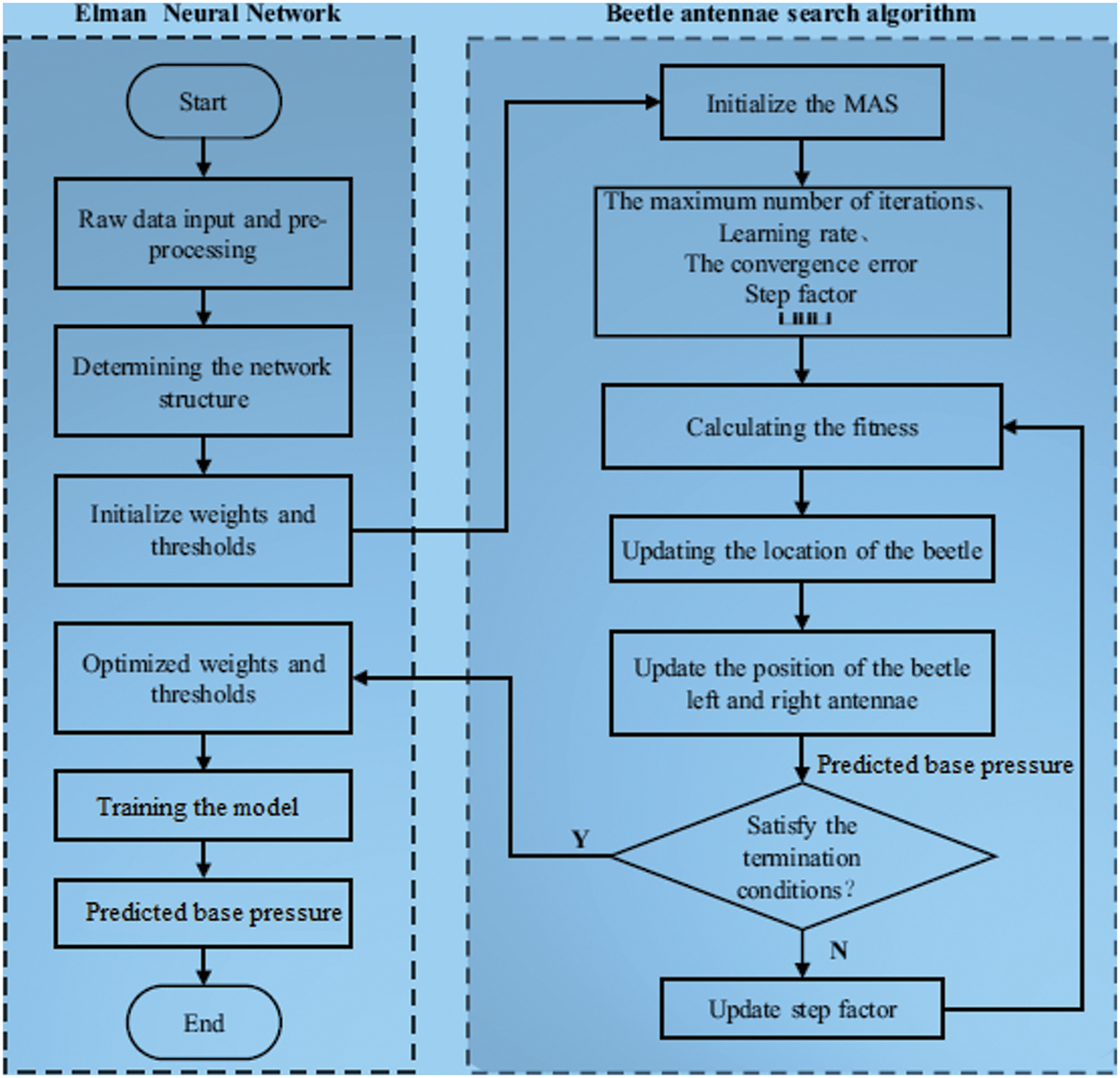
Figure 4: BAS-ENN algorithm flow chart

Step 1: Compute the Elman NN model’s topology and dimensional vector. Assume the suggested model is I-H-O. The neuron numbers in the model’s IL, HL, and OL are denoted by I, H, and O, respectively. Eq. (12) is used to compute H, where is α value in the range [0–1] [30]. The weights of the Elman NN’s I-H-O, as well as the commencement of every individual neuron, generate a dimensional vector Sspace, which is computed by Eq. (13):

H=I+O+α(12)

Sspace=IH+HO+H+O(13)

Step 2: Set up the BAS algorithm’s settings. Calculate the spacing d0 between the either ends of the antennae of the beetle, the starting step size δ, the utmost iterations n, the learning goal convergence error c, then generate a random vector configurations using Eq. (7).

Step 3: Compute the FF and its value. As demonstrated in Eq. (10), the RMSE of the training dataset is utilized based on the FF criterion, and the FF value is determined.

Step 4: Updating the beetle location. Initially, using Eq. (8) the positions of the beetle’s antennae are calculated, and the fitness values of the antennae’s, i.e., f(xiright) and f(xileft)are then determined using Eq. (10). By comparing both values, the simplified center location xicenteris updated using Eq. (9). This automatically adjusts the weights of the ENN, updates the dimensions of the solution, and determines the current coordinates of the FF.

Step 5: Stop the judgment by iterating. Evaluate if the fitness function value is accurate enough. If a significant level of accuracy is obtained after the completion of iterations, proceed over to Step 6; if not, Step 4 is repeated.

Step 6: Model training and optimal solution creation. The optimum initial weights and thresholds for Elman NN training are found once the BAS algorithm finishes iterating, and this response is used to train the Elman NN until the model’s training accuracy is reached.

Step 7: A unique test set is used to forecast the model to be trained.

The trained model forecasts for the fresh test set. The calculations are performed for this specified test set, and the findings obtained are output.

3.3 Base Pressure Prediction Based on the PCA‑BAS‑ENN Model

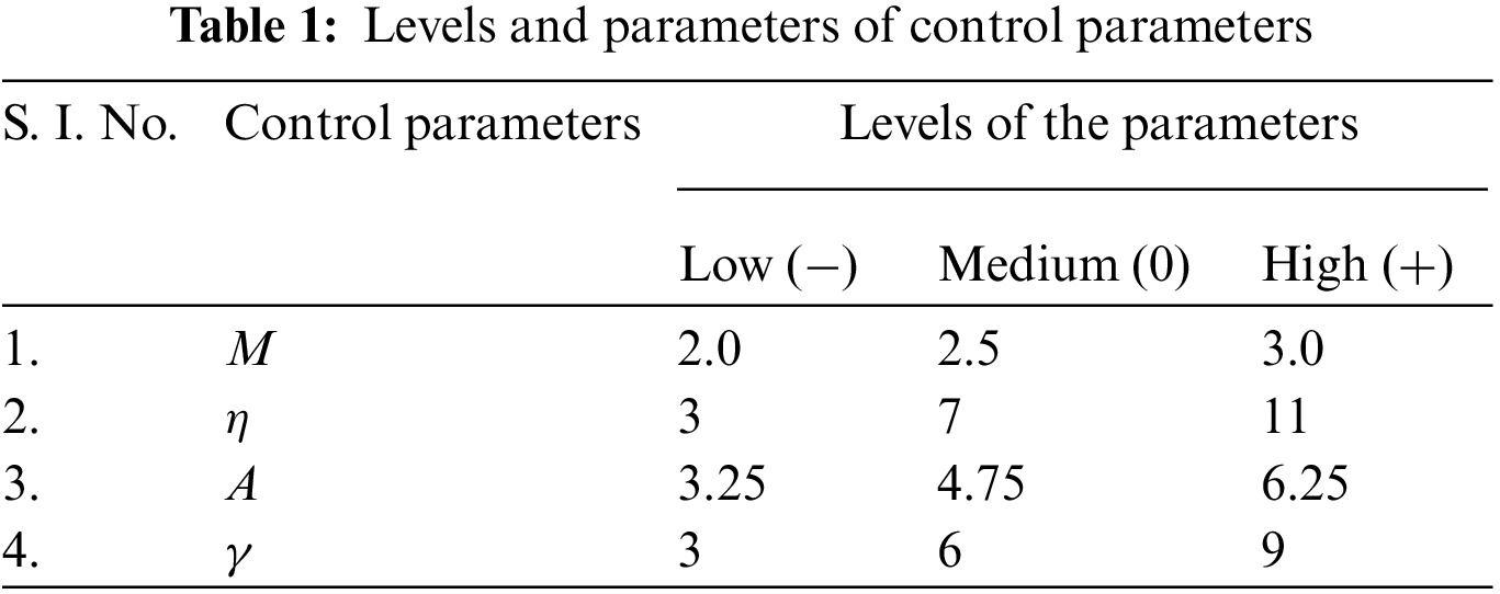
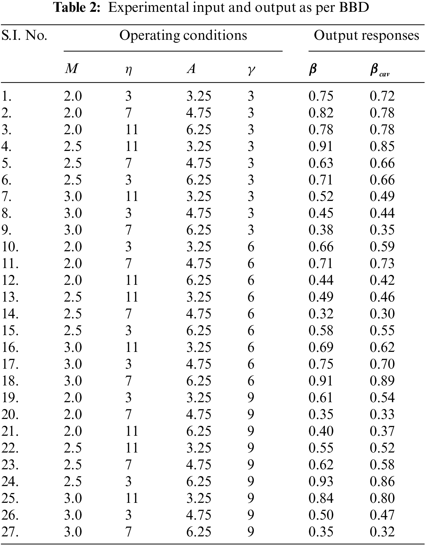
According to the literature, the parameters influencing the suddenly expanded flow process are numerous and complicated. However, in the flow process, M may be selected before experimentation. η, α, γ, and cavity dimensions in the expanded flow process are the other important parameters. Table 1 summarizes the control parameters of the model. For training and testing, data were generated using the Box-Behnken Design (BBD) of response surface methodology (RSM) as shown in Table 2. A MATLAB software was used for this purpose. In response surface methodology (RSM), multiple factors and their interactions are taken into consideration using different experimental designs such as, central composite design (CCD), and Box-Behnken design (BBD), etc. [34]. These designs plan the number of experiments according to the number of parameters and their levels, and as a result develop non-linear regression equations. A statistical Minitab software is used for this purpose. For our study, the BBD was found suitable as per (Quadros et al. [34]). The experimental data have been used to generate nonlinear regression equations that create huge amounts of data required for training and testing. The non-linear regression equations indicate the distribution of the distinctive factors and variables that influence the β to a certain degree.

The actual β values developed from the nonlinear regression equation for different cases exhibit a chaotic distribution, thereby projecting that the data used for developing a model to predict β for such a flow process is accurate enough. The β results from the regression equation (see Eqs. (14a) and (14b)) were accurate upto ±7.45%. There would inevitably be some poor data points since most of the process parameters tend to vary in the regression equation. To enhance the model’s forecasting skills, this study applies the Pauta criteria to remove the erroneous data elements from the observed dataset in the manner shown in Eqs. (15)–(17).

(β)=−0.239+(0.205×M)−(0.191×η)−(0.378×α)−(0.252×γ)+(0.0506×M2)+(0.00805×η2)−(0.03458×α2)+(0.02815×γ2)+(0.03770×M×η)−(0.03901×M×α)−(0.02351×M×γ)−(0.02005×η×α)+(0.00789×η×γ)−(0.00450×α×γ)(14a)

(βcav)=−0.250+(0.121×M)−(0.134×η)−(0.401×α)−(0.301×γ)+(0.0492×M2)+(0.00768×η2)−(0.04591×α2)+(0.03120×γ2)+(0.02908×M×η)−(0.04919×M×α)−(0.03658×M×γ)−(0.03129×η×α)+(0.00891×η×γ)−(0.00711×α×γ)(14b)

|xi−μ|>3σ(15)

σ=1n∑i=1n(xi−μ)2(16)

μ=1n∑i=1nxi(17)

The confidence intervals [μ−3σ,μ+3σ] are the projected ranges of all the control parameters represented by μ and σ of the dataset, therefore excluding the samples referring to data beyond the interval. The five-spot triple smoothing approach was then used to smooth the regression dataset by Deng et al. [35]. Fig. 5 displays the smoothed findings partially.

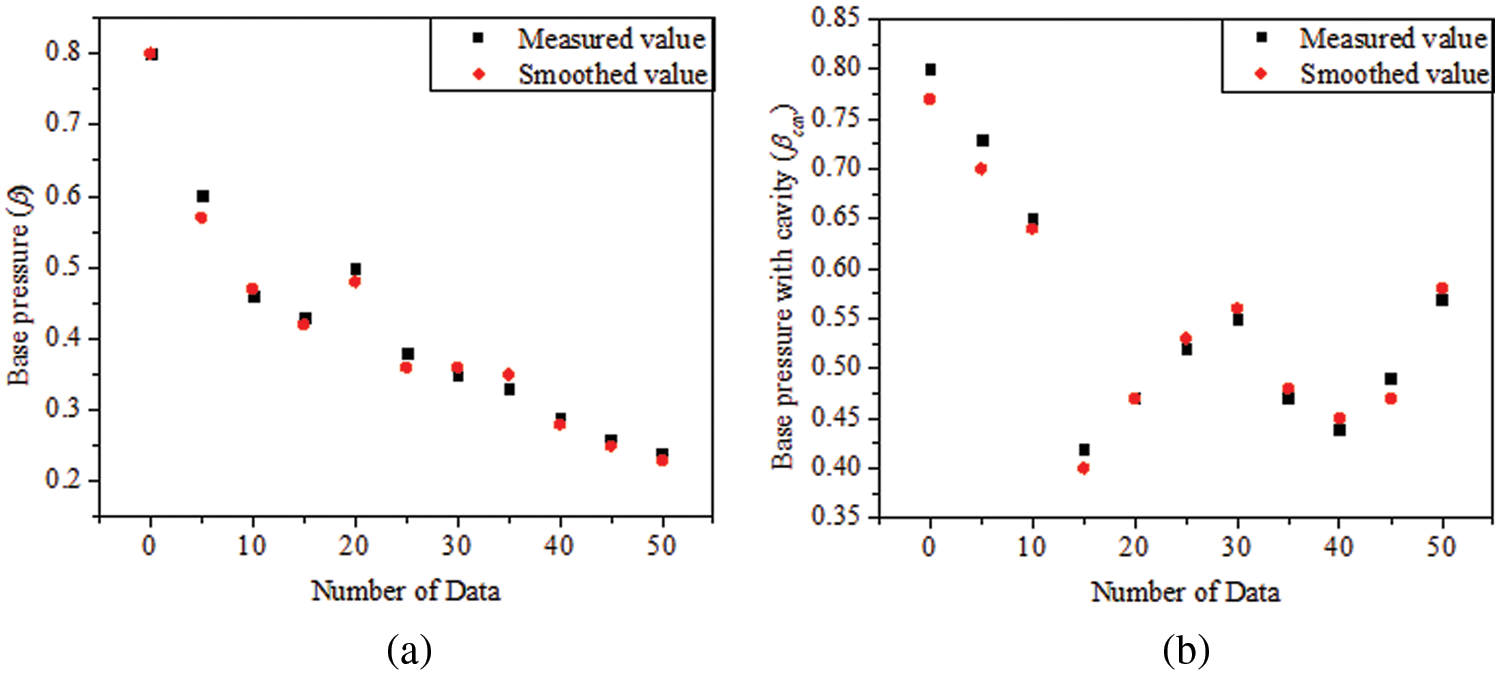
Figure 5: Five-spot triple smoothing

4  Results and Discussion

4.1 Base Pressure Analysis

Before the NN analysis, we must understand the behavior of base pressure for the different parameters. For this purpose, variation of β w.r.t. M, η, α, and γ has been studied thoroughly. The experimental results were normalized with atmospheric pressure. Fig. 6a shows the variation of β and the influence of cavity on β for a changing γ, for different values of η. It is observed that β decreased significantly as η increased, and marginally reduces for increasing γ. For the current range of η implemented, the flow for Mach 2.0 was correctly expanded and over-expanded for Mach 2.5 and 3.0. For nozzles that are over-expanded, the pressure gradient is always adverse, which tends to decrease β for an increasing η. This trend is seen in Fig. 6a, that shows the β variation for a constant Mach of 2.5. The over-expansion increases with increase in Mach numbers, and the flow exiting the nozzle duct interface possesses an oblique shock. This causes wave motions across the flow area that eventually makes the flow field oscillatory [8]. As η is increased, the flow tends to become under-expanded reducing the level of over-expansion, and the nozzle experiences an improved pressure difference leading to a decreasing trend in β.

Figure 6: Variation of β w.r.t., (a) γ; (b) M

It is important to note that, a higher value for β is observed when the α is high as seen in Fig. 6b. The relief available for the flow to recirculate (Fig. 1) is generally dictated by α. As α increases, development of powerful suction at the base takes place for a fixed intensity of the primary vortex. This primary vortex intensity apparently regulates the pressure in the base region. It creates a low pressure region at the base, prior to the flow reaching its reattachment point causing influx of additional flow from the walls into the base region [1]. The additional flow developed captures the base region causing the main the flow to get disturbed. This diminishes the intensity of the primary vortex. This reduction causes the β levels to increase to an extent such that, any additional mass incurrance would not be possible into the base region [8]. Therefore, effectiveness of the vortex is reduced, thereby increasing β. The induction of a cavity into the expanded duct showed that the level of β significantly decreased for all cases of the current study. As per Vijayaraj et al. [6], inducing a cavity or rib generates secondary vortices within the duct. These secondary vortices influence mixing, making the flow field oscillatory, thereby modifying the strength of the primary vortex [1]. As a result, β is reduced to a significant level.

The model contains multiple input parameters, as indicated in Table 1, and these parameters are interconnected. Assume that these are the input variables for explicitely constructing the β preset model. In that condition, the number of model operations would rise, as will the forecast inaccuracy, resulting in the phenomena known as ‘dimensional disaster’. Fig. 7 depicts the computation results, which demonstrate that the combined significance of the initial 45 principal elements reaches 88.90% (commonly, a cumulative significance rate greater than 85% is preferred), so the initial 45 principal elements are chosen to substitute the existing parameters as fresh input variables to establish the β preset model.

Figure 7: Five-spot triple smoothing

4.2 Performance Analysis of Models

To evaluate the performance of various algorithms on the β presetting model, the GA-BP and PSO-BP algorithms are compared with the PCA-BAS-ENN under identical data settings. Numerous results for β were developed using the regression equation that was utilized in all three NN models, and the results are shown in Table 3. Here, T is the highest time required for training, a is the convergence precision, S is the population size, l is the learning rate, Pc is crossover probability, i is maximum iterations, c1 and c2 are the learning parameters that have the highest and lowest levels, respectively, Pm is the mutation probability, v is the highest velocity of the particle, δs and d0 are defined earlier in Eqs. (11) and (6), respectively.

Meanwhile, three performances of MAE, MAPE, and RMSE are chosen as the performance criteria in this paper to extensively and categorically analyze the predictive performance and computational efficiency of each model mentioned above. The formulae are presented below in Eqs. (18)–(20) (Song et al. [27]):

MAE=1n∑i=1n|yipre−yiact|(18)

MAPE=1n∑i=1n|yipre−yiactyiact|×100%(19)

RMSE=1n∑i=1n(yipre−yiact)2(20)

where, yipre and yiact are the predicted and actual values. Table 4 displays the efficiency of the above three models' training and testing sets for β prediction results. Depending on the values obtained in Table 4, Fig. 8 depicts the error differences of MAE, MAPE, and RMSE, respectively.

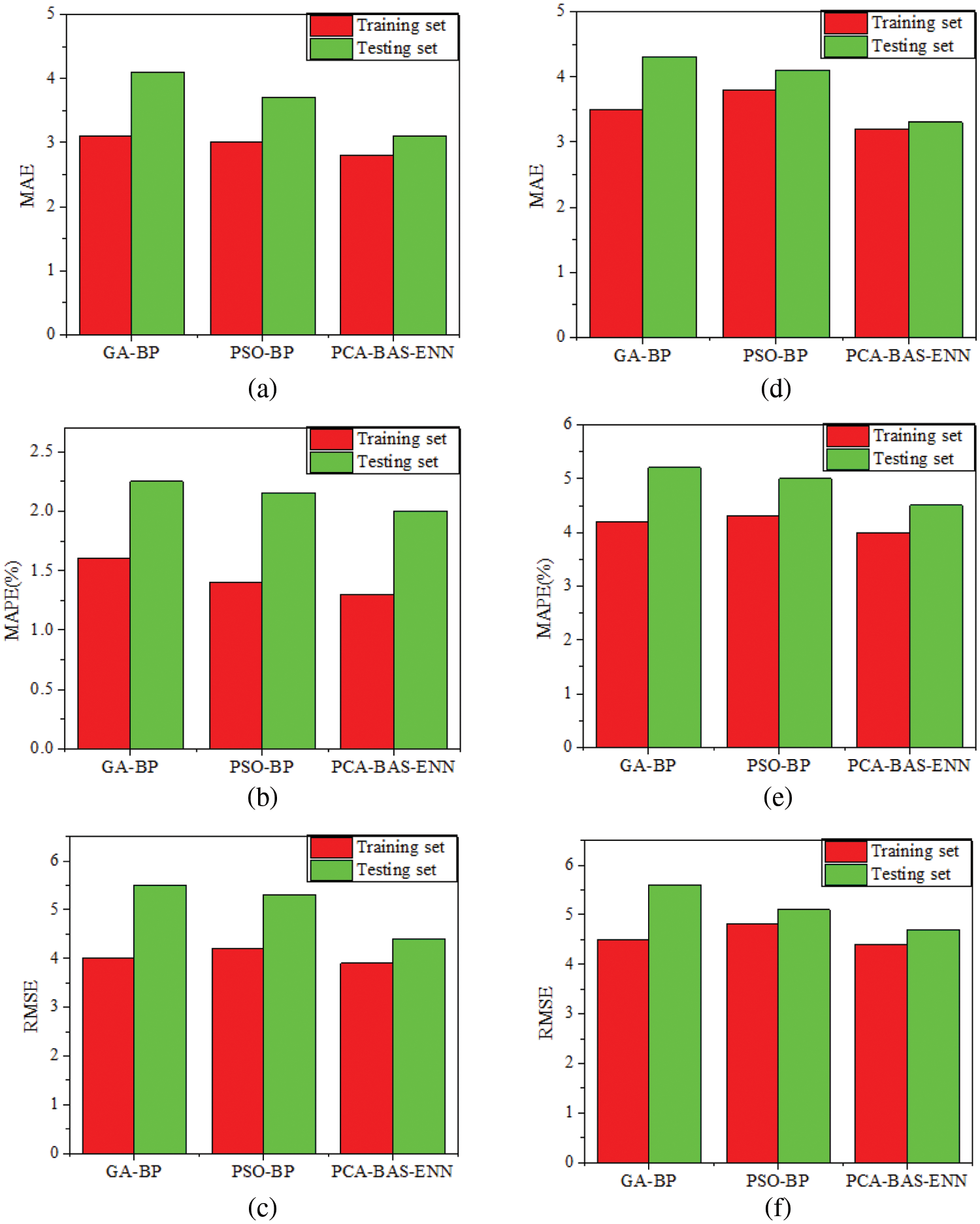
Figure 8: Error comparison of the three models. (a–c) for β; (d–f) for βcav

From Table 4 and Fig. 8, the following points may be concluded: On the training set, the PCA-BAS-ENN models’ three error indicators for predicting β are much lower compared to the rest of the models. When comparing the PSO-BP model to the GA-BP model, the precision of the former model was high for predicting β, whereas the latter had a better ability to predict βcav. In comparison to the GA-BP model, the test data points were close to the PSO-BP model for all the β prediction indicators. All in all, the GA-BP model performed poorly and was unstable. In both the training and testing data sets, the performance of the PCA-BAS-ENN model is best when compared to the other two models.

The primary reason for the poor performance of the GA-BP model (Fig. 8) in prediction of β was mainly due to the fact that, the GA-BP model has the tendency to get stuck at local minima. Here, the model converges to a suboptimal solution beyond which, it cannot progress further to find a better solution. This problem occurs due to improper tuning of the GA-BP parameters [27]. Parameter tuning is challenging process as it requires significant expertise and experimentation. Additionally, the GA-BP model predominantly relies on the combination of genetic algorithm and back propagation algorithm. The weights and baises of the model tend to get optimized automatically, leading to inaccurte predictions. On the other hand, the PCA-BAS-ENN model performed best as it executed multiple functions that include, reduction of dimensionality of input data by transforming variables into tiny principal components undertaken by PCA, optimization of NN parameters that lead to faster convergence and better performance by BAS (which is an algorithm based on hunting behavior of ant lions); the ENN uses the hidden layer to otimize the training process. The PSO-BP model that performed slightly better than the GA-BP model especially for the testing data, is a global optimization model that has the ability to find the global minima without getting stuck at local minima [28,29]. Therefore, it performed better with more accurate predictions.

4.3 Comparison of the Prediction Results of All Three Models

Fig. 9 shows the comparison of performance prediction of all three models for the testing data set. Each models’ performance is determined by the set of data points that fall within the three-error band (TEB), which represents an absolute error of ≤0.05. An increase in the number of data points that fall beyond the TEB indicates the poor performance of the model. From Figs. 9a–9c, the absolute error for prediction of β by the ENN model is the best as only three of its data points lie beyond the TEB. Quite a few deviation points have been observed to lie outside the TEB for the PSO-BP and GA-BP models, thereby reducing their prediction ability significantly. From Figs. 9d–9f, the comparison led to the same conclusions. Overall, it can be thoroughly construed that the PCA-BAS-ENN model had the best prediction ability for β, closing in with its actual value.

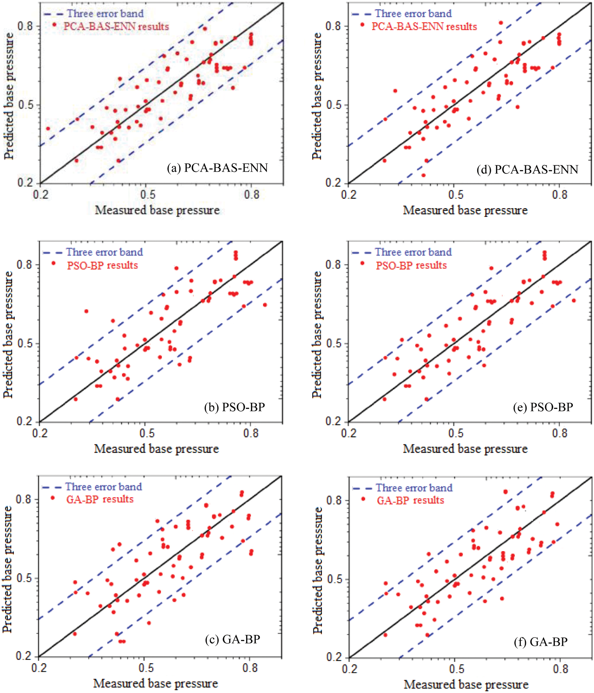
Figure 9: Comparison of performance prediction for all the three models. (a–c) for β; (d–f) for βcav

The hybrid PCA-BAS-ENN model as seen in Figs. 9a and 9d achieves a low training error due to less deviation, indicating that the model fits the training data very well. The ability of the PCA-BAS-ENN model to perform well in the TEB is due to its robustness and generalization ability. The models ability to reduce input variable dimensionality [27], optimize parameters using the BAS algorithm, and handle various other noise and outliers are the primary reasons that make it a powerfull tool to forecast the β and βcav for a supersonic suddenly expanded flow process.

The frequency distribution of the absolute error has been presented in Fig. 10. This type of frequency distribution is plotted as an x-y plot wherein, x-axis represents the absolute error value and y-axis represents the frequency of each error. The model here is said to perform well when its distribution is centered around zero with relatively few errors of high magnitude. Similarly, the model performs poorly when the distribution is spread and sees larger errors of higher magnitude. It can be seen that the errors associated with the PCA-BAS-ENN model prediction are highly pronounced in the 0 range. This is primarily due to reduction of dimensionality of the input data, that moderates the complexity of the data leading to a faster training process [27]. This signifies that there are less significant prediction error samples in this model in comparison to the other two models, thereby confirming that the model is highly secure, balanced and error-tolerant.

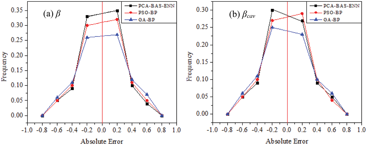
Figure 10: Frequancy distribution of asbsolute errors for (a) β, and (b) βcav

The theoretical β in missiles and projectiles and combustion chambers as a part of practical field application is determined through the uncertainty analysis. This analysis is developed based on values of control pressure and exit pressure that are required for the functioning of an actual aerodynamic problem [3,8]. This is performed to validate the positive influence of the model with the best prediction ability, suggested in this study. The comparison of β accuracy before and after optimization in a suddenly expanded axisymmetric duct is shown in Fig. 11. The results show a significant improvement in the average β deviation from 93.655% to 95.590%, which eventually improves the β control deviation. According to the β data obtained, we compared the second-order and the fifth-order base pressure targets and determined the RMSE for comparison.

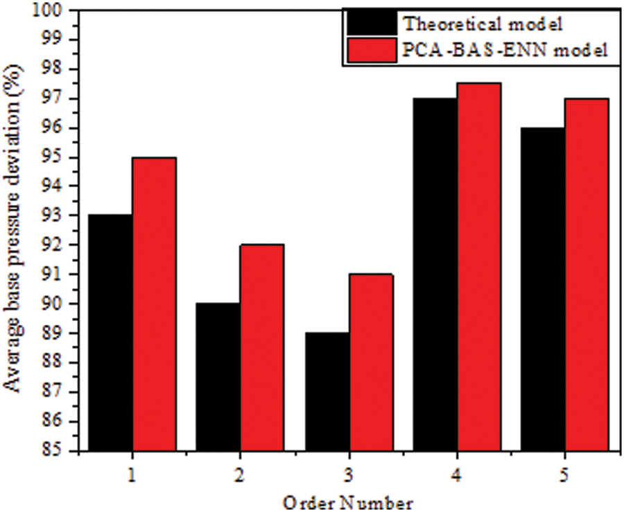
Figure 11: Comparison of base pressure values for varying model settings

(RMSE)2=∑j=1n(B2na−B2ng)2/n(21)

(RMSE)5=∑j=1n(B5na−B5ng)2/n(22)

Here, n is the sample number, B2a and B5a are measured β values of 2nd and 5th order Mach numbers, respectively; B2g and B5g are target β values of 2nd and 5th order Mach values, respectively; δ2 and δ5 are RMSE of 2nd and 5th order measured β values, respectively. As per Fig. 12, for the same Mach value, the average δ was 0.396 and 0.477 for the 2nd and 5th order β, respectively. After the application of the PCE-BAS-ENN model, the average RMSE for the 2nd and 5th order base pressure was 0.341 and 0.393, respectively. This means that the average RMSE reduced by 0.055 (13.88%) and 0.084 (17.61%), respectively.

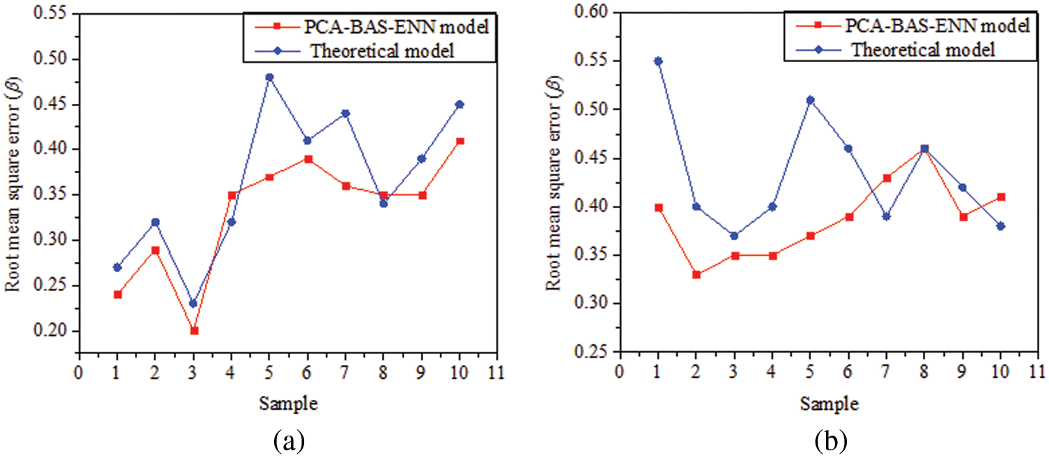
Figure 12: Comparison of base pressure for different models. (a) 2-order, (b) 5-order

5  Conclusions

Supersonic expanded flow process has been found to be very handy in regulating the base drag of aerodynamic vehicles. Numerous experimental and numerical investigations carried out by researchers previously, supported the implementation of internal modifications in the abruptly expanded duct in order to achieve favourable performance characteristics. However, analyzing such flows for a number of input parameters becomes time-consuming, challenging, and expensive. In this regard, the use of machine learning models in non-linear fluid flow problems still remains unexplored. Therefore, the current study developed a data-driven forecasting model by employing the PCA and BAS-ENN algorithms to determine the optimal setting of β in a suddenly enlarged flow process. The experimental examination along with the NN analysis in this work led to the following results:

•   β reduces considerably for increasing η and marginally reduces for increasing γ due to the production of an oblique shock that causes the flowing nature to be wave-dominated.

•   The induction of a cavity into the expanded duct decreased β significantly, due to the introduction of secondary vortices, that make the flow field oscillatory.

•   Under identical settings, the PCA-BAS-ENN model was compared to the other two algorithms, for determining β, and it was discovered that the former has the best forecasting performance and accuracy. This machine learning algorithm is efficient in estimating β, while ignoring the constraints of the GA, like inadequate local search capabilities, early maturity, and deficient model efficiency due to genetic variation randomness; it also excludes the drawbacks of the BP NN algorithm, such as slowness of calculation and the simplicity of slipping into localized extremes.

•   Upon having integrated with the PCA-BAS-ENN model, the practical field implementation displays that the average β deviation increased from 93.655% to 95.590%, which eventually improved the β control deviation. The average δ between the 2nd and 5th order β was reduced by 0.055 (13.88%) and 0.084 (17.61%), respectively. This finding suggents that effectiveness of control management is good following the use of the new β preset models.

•   All the machine learning models of the present study for β and βcav have shown the ability to predict the data successfully. Mathematical modelling is very complex for such type of research due to the data being highly non-linear. Such algorithms could be used to deal with several fluid flow problems of this kind. In the current study, the models employed will help aerodynamic engineers forecast the inception and advancement of base drag across a high-speed aerodynamic vehicle without the use of any experiments or simulation. This would eliminate the necessity of any prior insight or expertise of the flow process. Ultimately, this would result in less use of energy and material, also excluding the method of trial and error generally used to determine the optimal combination of process parameters that control base drag.

Acknowledgement: The authors acknowledge the support of Prince Sultan University for paying the article processing charges (APC) of this publication.

Funding Statement: This research is supported by the Structures and Materials (S&M) Research Lab of Prince Sultan University.

Conflicts of Interest: The authors declare that they have no conflicts of interest to report regarding the present study.

References

1. Rathakrishnan, E. (2001). Effect of ribs on suddenly expanded flows. American Institute Astronautics and Aeronautics Journal, 9(7), 1402–1404. https://doi.org/10.2514/2.1461 [Google Scholar] [CrossRef]

2. Afzal, A., Aabid, A., Ambareen, K., Khan, S. A., Upendra, R. et al. (2020). Response surface analysis, clustering, and random forest regression of pressure in suddenly expanded high speed aerodynamic flows. Aerospace Science and Technology, 107(1), 106318. https://doi.org/10.1016/j.ast.2020.106318 [Google Scholar] [CrossRef]

3. Khan, S. A., Rathakrishnan, E. (2002). Active control of suddenly expanded flows from over expanded nozzles. International Journal of Turbo and Jet Engines, 19(1–2), 119–126. https://doi.org/10.1515/TJJ.2002.19.1-2.119 [Google Scholar] [CrossRef]

4. Pandey, K. M., Rathakrishnan, E. (2006). Annular cavities for base flow control. International Journal of Turbo and Jet Engines, 23(2), 113–127. https://doi.org/10.1515/TJJ.2006.23.2.113 [Google Scholar] [CrossRef]

5. Sandeep, Y., Ashish, V., Vijayaraja, K., Rathakrishnan, E. (2008). Base pressure control by using ribs in subsonic and sonic suddenly expanded flows. 2nd International Conference on Recent Advances in Experimental Fluid Mechanics, Vijayawada, India. [Google Scholar]

6. Vijayaraja, K., Elongovan, S., Rathakrishnan, E. (2008). Effect of rib on suddenly expanded supersonic flow. International Review of Aerospace Engineering, 39(7), 196–199. https://doi.org/10.2514/2.1461 [Google Scholar] [CrossRef]

7. Baig, M. A. A., Al-Mufadi, F., Khan, S. A., Rathakrishnan, E. (2011). Control of base flows with micro jets. International Journal of Turbo and Jet Engines, 28(1), 259–269. https://doi.org/10.1515/tjj.2011.009 [Google Scholar] [CrossRef]

8. Khan, S. A., Rathakrishnan, E. (2003). Control of suddenly expanded flows with micro jets. International Journal of Turbo and Jet Engines, 20(1), 63–81. https://doi.org/10.1515/TJJ.2003.20.1.63 [Google Scholar] [CrossRef]

9. Fharukh, A. G. M., Alrobaian, A. A., Aabid, A., Khan, S. A. (2018). Numerical analysis of convergent-divergent nozzle using finite element method. International Journal of Mechanical and Production Engineering and Development, 8(6), 373–382. https://doi.org/10.24247/ijmperddec201842 [Google Scholar] [CrossRef]

10. Sajali, M. F. M., Aabid, A., Khan, S. A., Mehaboobali, F. A. G., Sulaeman, E. (2019). Numerical investigation of flow field of a non-circular cylinder. CFD Letters, 11(5), 37–49. [Google Scholar]

11. Aabid, A., Nabilah, L., Khairulaman, B., Khan, S. A. (2021). Analysis of flows and prediction of CH10 airfoil for unmanned arial vehicle wing design. Advances in Aircraft and Spacecraft Science, 8(2), 24–35. https://doi.org/10.12989/aas.2021.8.2.087 [Google Scholar] [CrossRef]

12. Sajali, M. F. M., Ashfaq, S., Aabid, A., Khan, S. A. (2019). Simulation of effect of various distances between front and rear body on drag of a non-circular cylinder. Journal of Advanced Research in Fluid Mechanics and Thermal Sciences, 62(1), 53–65. [Google Scholar]

13. Cameron, R. N., Semih, M. Ö., Daniel, R. L., Keith, W. (2008). Supersonic, variable-throat, blow-down wind tunnel control using genetic algorithms, neural networks, and gain scheduled PID. Applied Intelligence, 29(1), 79–89. https://doi.org/10.1007/s10489-007-0082-y [Google Scholar] [CrossRef]

14. Zhang, D., Liang, Y., Dong, H. (2023). Dendritic cell algorithm with grouping genetic algorithm for input signal generation. Computer Modeling in Engineering & Sciences, 135(3), 2025–2045. https://doi.org/10.32604/cmes.2023.022864 [Google Scholar] [CrossRef]

15. Quadros, J. D., Khan, S. A., Sapkota, S., Vikram, J., Prashanth, T. (2020). On recirculation region length of suddenly expanded supersonic flows, using CFD and fuzzy logic. International Journal of Computational Fluid Dynamics, 34(10), 757–773. https://doi.org/10.1080/10618562.2020.1828580 [Google Scholar] [CrossRef]

16. Quadros, J. D., Khan, S. A. (2020). Prediction of base pressure in a suddenly expanded flow process at supersonic Mach number regimes using ANN and CFD. Journal of Applied Fluid Mechanics, 13(2), 499–511. https://doi.org/10.29252/jafm.13.02.30049 [Google Scholar] [CrossRef]

17. Aabid, A., Khan, S. A. (2020). Investigation of high-speed flow control from C-D nozzle using design of experiments and CFD methods. Arabian Journal of Science and Engineering, 46(3), 2201–2230. https://doi.org/10.1007/s13369-020-05042-z [Google Scholar] [CrossRef]

18. Han, H., Wang, W. (2023). A hybrid BPNN-GARF-SVR prediction model based on EEMD for ship motion. Computer Modeling in Engineering & Sciences, 134(2), 1353–1370. https://doi.org/10.32604/cmes.2022.021494 [Google Scholar] [CrossRef]

19. Afzal, A., Khan, S. A., Islam, T. M., Jilte, R. D., Ambareen, K. et al. (2020). Investigation and back-propagation modeling of base pressure at sonic and supersonic Mach numbers. Physics of Fluids, 32(9), 096109. https://doi.org/10.1063/5.0022015 [Google Scholar] [CrossRef]

20. Aabid, A., Khan, S. A., Afzal, A., Baig, M. (2021). Investigation of tiny jet locations effect in a sudden expansion duct for high-speed flows control using experimental and optimization methods. Meccanica, 6(1), 17–42. https://doi.org/10.1007/s11012-021-01449-6 [Google Scholar] [CrossRef]

21. Al-khalifah, T., Aabid, A., Khan, S. A., Bin Azami, M. H., Baig, M. (2019). Response surface analysis of the nozzle flow parameters at supersonic flow through microjets. Australian Journal of Mechanical Engineering, 13(2), 1–15. https://doi.org/10.1080/14484846.2021.1938954 [Google Scholar] [CrossRef]

22. Quadros, J. D., Nagpal, C., Khan, S. A., Aabid, A., Baig, M. (2022). Investigation of suddenly expanded flows at subsonic Mach numbers using an artificial neural networks approach. PLoS One, 17(10), 1–28. https://doi.org/10.1371/journal.pone.0276074 [Google Scholar] [PubMed] [CrossRef]

23. Quadros, J. D., Suhas Khan, S. A., Aabid, A., Baig, M. (2022). Fuzzy-based prediction for suddenly expanded axisymmetric nozzle flows with microjets. Bulletin of Polish Academy of Technical Sciences, 70(5), 1–11. https://doi.org/10.24425/bpasts.2022.142654 [Google Scholar] [CrossRef]

24. Genick, B. M. (2007). Gas dynamics tables. Version 1.3. https://doi.org/10.5281/zenodo.5523531 [Google Scholar] [CrossRef]

25. Yang, L., Wang, F., Zhang, J. J., Ren, W. H. (2019). Remaining useful life prediction of ultrasonic motor based on Elman neural network with improved particle swarm optimization. Measurement, 143, 27–38. https://doi.org/10.1016/j.measurement.2019.05.013 [Google Scholar] [CrossRef]

26. Wei, L., Wu, Y. Q., Fu, H., Yin, Y. P. (2018). Modeling and simulation of gas emission based on recursive modified Elman neural network. Mathematical Problems in Engineering, 2018(1), 1–10. https://doi.org/10.1155/2018/9013839 [Google Scholar] [CrossRef]

27. Song, L. B., Xu, D., Wang, X. C., Yang, Q., Ji, Y. F. (2022). Application of machine learning to predict and diagnose for hot-rolled strip crown. International Journal of Advanced Manufacturing Technology, 120(1–2), 881–890. https://doi.org/10.1007/s00170-022-08825-w [Google Scholar] [CrossRef]

28. Jiang, X. Y., Lin, Z. Y., He, T. H., Ma, X. J., Ma, S. et al. (2020). Optimal path finding with beetle antennae search algorithm by using ant colony optimization initialization and different searching strategies. IEEE Access, 8, 15459–15471. https://doi.org/10.1109/ACCESS.2020.2965579 [Google Scholar] [CrossRef]

29. Jiang, X. Y., Li, S. (2017). BAS: Beetle antennae search algorithm for optimization problems. International Journal of Robotics and Control, 1(1), 1–5. https://doi.org/10.5430/ijrc.v1n1p1 [Google Scholar] [CrossRef]

30. Wang, Z. H., Gong, D. Y., Li, X., Li, G. T., Zhang, D. H. (2017). Prediction of bending force in the hot strip rolling process using artificial neural network and genetic algorithm (ANN-GA). International Journal of Advanced Manufacturing Technology, 93(9–12), 3325–3338. https://doi.org/10.1007/s00170-017-0711-5 [Google Scholar] [CrossRef]

31. Jiang, X. Y., Li, S. (2017). Beetle antennae search without parameter tuning (BAS-WPT) for multi-objective optimization. Filomat, 34(15), 5113–5119. https://doi.org/10.2298/FIL2015113J [Google Scholar] [CrossRef]

32. Lin, Z. Y., Ma, S., Ma, X. J., Jiang, X. Y., Li, S. (2018). Two new beetle antennae search (BAS) algorithms and their comparative investigation. International Journal of Robotics and Control, 2(1), 9–17. https://doi.org/10.5430/ijrc.v2n1p9 [Google Scholar] [CrossRef]

33. Yue, Z. C., Li, G., Jiang, X. Y., Li, S., Chen, J. et al. (2020). A hardware descriptive approach to beetle antennae search. IEEE Access, 8, 89059–89070. https://doi.org/10.1109/ACCESS.2020.2993600 [Google Scholar] [CrossRef]

34. Quadros, J. D., Khan, S. A., Antony, A. J. (2018). Modelling of suddenly expanded flow process in the Supersonic Mach number regime using DOE and RSM. Journal of Computational Applied Mechanics, 49(1), 149–160. https://doi.org/10.22059/jcamech.2018.248043.221 [Google Scholar] [CrossRef]

35. Deng, J. F., Sun, J., Peng, W., Hu, Y. H., Zhang, D. H. (2019). Application of neural networks for predicting hot-rolled strip crown. Applied Soft Computing, 78, 119–131. https://doi.org/10.1016/j.asoc.2019.02.030 [Google Scholar] [CrossRef]