Improved RRT^∗ Algorithm for Automatic Charging Robot Obstacle Avoidance Path Planning in Complex Environments

1  Introduction

With the rapid development of driverless and electric vehicles, electric vehicles have become a significant research hit in automatic charging [1,2]. The current research on automatic charging automated arms mainly includes visual calibration [3], trajectory planning [4,5], motion control [6], and obstacle avoidance [7]. In addition, automated arm obstacle avoidance time is also considered in the field of automatic charging, so it is crucial to study the optimal planning time for robotic arm obstacle avoidance. However, due to the coupling between the automated arm linkages, which cannot be considered as mass points, the planning needs to detect the arm collision at each position, which makes planning difficult and takes a long time. Therefore, it is crucial to research ways to decrease the time cost of automated arm path planning and the route cost of automated arm motion to lower the energy consumption and wear of automated arm motion and adapt to application situations requiring greater speed.

Contemporary scholars have done a great deal of research on the methods and strategies of robotic arm path planning [8]. In recent years, more scholars have chosen to map the arm shape into Cartesian space to complete the robotic arm path planning [9]. The commonly used path planning methods in Cartesian space are the artificial potential field method [10], the ant colony algorithm [11,12], and the A* algorithm [13]. However, these methods each have their weaknesses: local property of artificial potential planning time of A* algorithm. These methods are more suitable for the path planning of mobile robots in two-dimensional maps, and the operation is complicated and time-consuming in the high-dimensional space of robotic arms. To solve path plans in high-dimensional space, LaValle [14] first proposed the Rapidly exploring Random Trees, RRT. The algorithm can quickly sample in high dimensional spaces without modeling due to its random sampling mechanism and has the integrity to explore directional probabilities. However, its expansion may be off the target direction, so convergence is slow. Salzman et al. [15] proposed an improved learning method to address the problems of the RRT algorithm, such as low search efficiency. The shortest path is introduced into the RRT algorithm as a distance metric to speed up planning and shorten the path distance. Experimental results show that the method shortens the planning time and path length. But there are plenty of iteration points. Jeong et al. [16] proposed a Quick-RRT* algorithm to address the problem of slow convergence of the RRT* algorithm. It is shown experimentally that the algorithm can further improve performance by combining it with other sampling strategies. However, it has not been verified in the high dimensional environment, which cannot guarantee the good practicability of the manipulator. Wang et al. [17] proposed KB-RRT* algorithm. The method retains the advantage of bi-directional search, resulting in shorter paths. Simulation experiments show that KB-RRT* performs better in path length, achieving comparative performance in terms of the number of iterations and nodes compared to K-RRT. But the failure rate is higher in high dimensional environment. Yuan et al. [18] proposed an adaptive hybrid dynamic step size and target gravity path planning algorithm to address the problem of high randomness of RRT algorithm. The method improves the ability to pass through narrow passages as well as the forward speed. But the accuracy of the algorithm is low.

Current research on trajectory obstacle avoidance for automatic charging robots leaves much to be desired, such as the long movement time and the extended movement distance of some improved RRT* during trajectory obstacle avoidance. An improved RRT* algorithm is proposed in this paper to improve the efficiency of the RRT* algorithm in path planning. The main improvements are in the algorithm’s efficiency, the search time, and the path distance. And it can effectively solve the problems of many planning branches and low success rates in the complex environment of high-dimensional space. In addition, the proposed random tree node expansion control strategy improves the blindness of spontaneous tree node expansion; the proposed random tree node expansion capability detection strategy improves the convergence efficiency of the algorithm by reducing invalid nodes.

2  Research Content

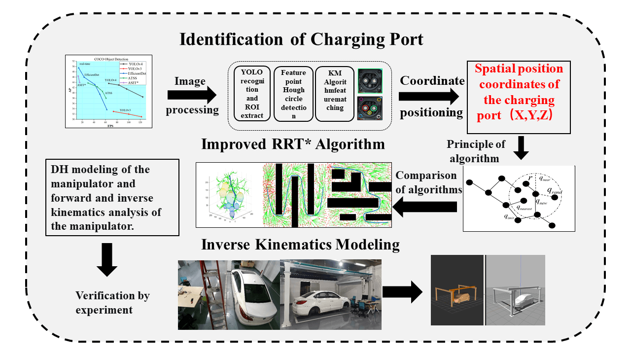
In this paper, we apply machine vision algorithms [19] to identify and locate new energy vehicles and charging ports through a self-designed robotic arm configuration and control system. It also combines kinematic characteristics to plan the movement trajectory and ultimately automate the charging operation. Fig. 1 shows this paper’s overall structure.

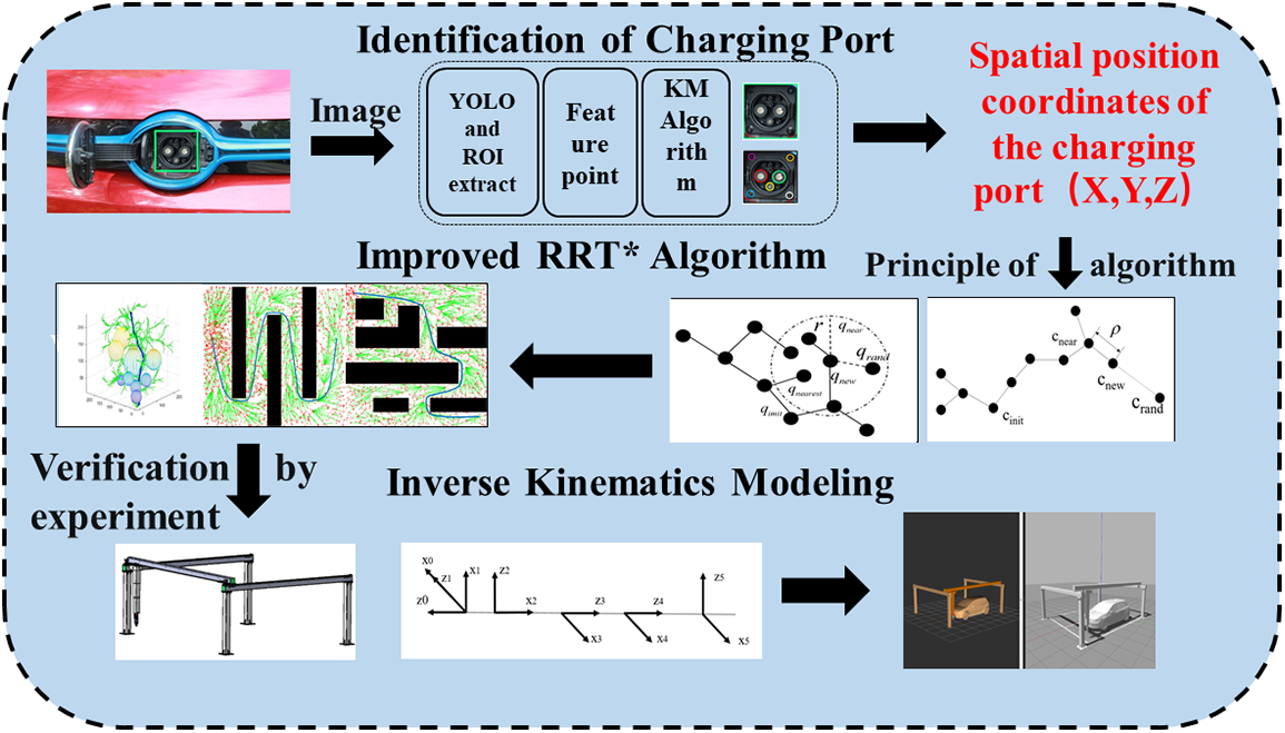
Figure 1: Framework of research content

Firstly, the charging port is roughly localized based on the automatic charging device by the homemade dataset, self-trained YOLOv4 target detection deep learning algorithm. Then the traditional image processing methods such as Hoff circle transform feature point extraction, KM feature matching algorithm, and single response matrix solution are used to precisely locate the charging port. The spatial position coordinates are obtained to provide the target position for the movement of the charging robot arm.

Secondly, the RRT* algorithm is improved to enable better obstacle avoidance for complex environments. The convergence times and path distances of the improved RRT* and RRT* and RRT in two and three dimensions are compared. The outcomes demonstrate that an improved RRT* algorithm may converge more quickly and precisely. Target points can be located rapidly.

Finally, the motion path of the charging robotic arm is planned based on the obtained vehicle charging port position. Forward and reverse kinematics analysis of the automatic charging device based on the D-H parameter method. Determine the transformation relationship between the end of the robotic arm and each joint variable of the robotic arm. D-H kinematic modeling of the automatic charging robotic arm based on the Matlab Robotics Toolbox and verification of its workspace accuracy. Finally, experimental verification was conducted to finally achieve accurate docking of the automatic charging.

3  Charging Port Identification and Positioning

Electric vehicles are to be charged automatically. The position of the vehicle charging port must first be determined. The identification and positioning of the vehicle charging port is part of a precise positioning process. The sensor used in the process is a local camera, and the calibrated camera captures the image of the vehicle’s charging port to be charged. The YOLO identification and ROI extraction, Hoff circle detection, and other image processing processes are completed to obtain the location information of the vehicle charging port and guide the charging gun to complete the docking with the charging port [20].

3.1 The YOLOv4 Target Detection Algorithm

The YOLOv4 algorithm [21] is chosen as the target detection algorithm due to its improved accuracy over YOLOv3. YOLOv4 uses many data enhancement methods and integrates more fully into the training process, while YOLOv5 has a smaller network and trains very quickly but is slightly less accurate than YOLOv4. YOLOv4 is an improved version of YOLOv3 that modifies the backbone network to achieve a balance between operation speed and detection accuracy. Fig. 2 shows the network structure of YOLOv4.

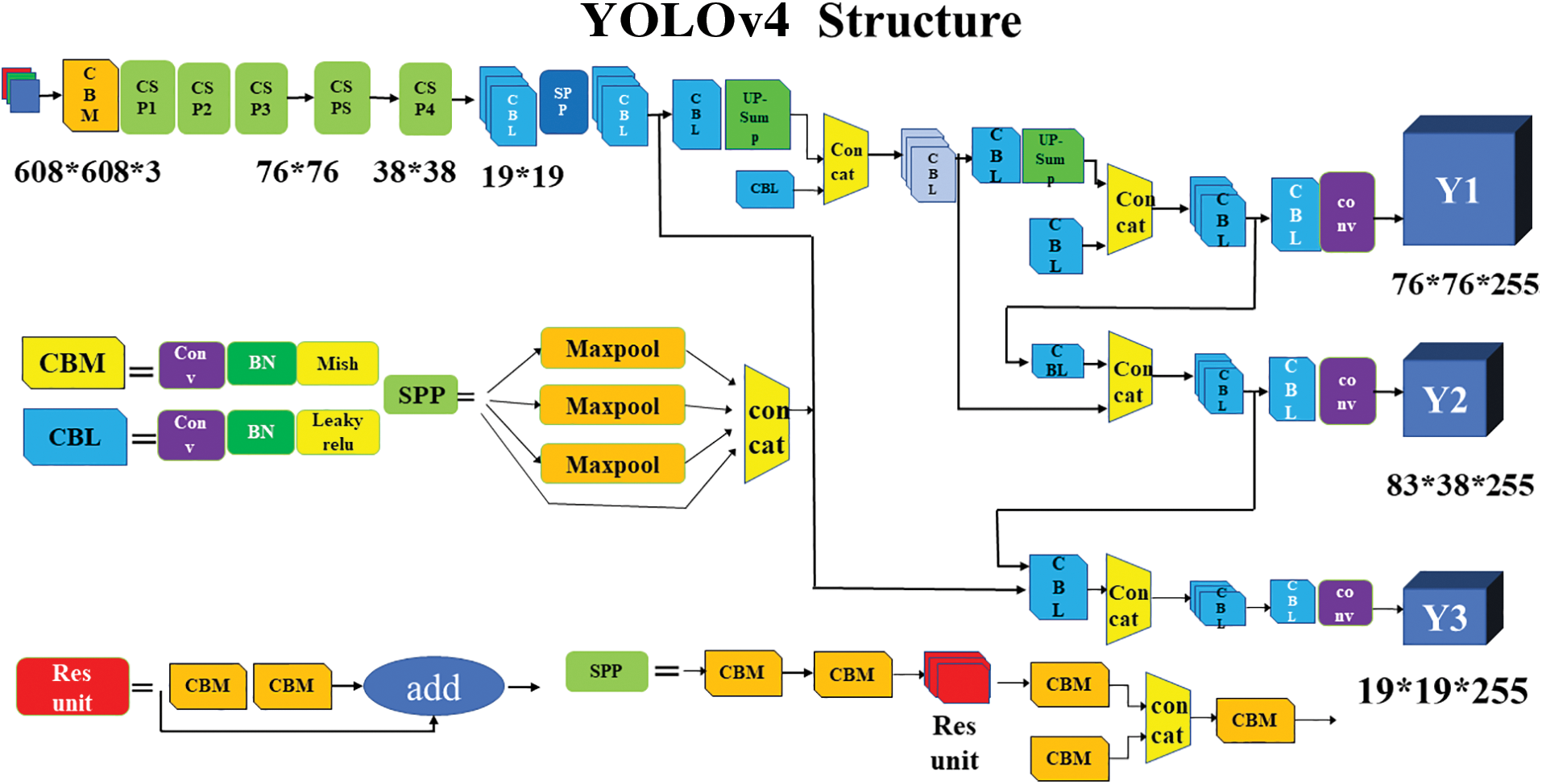
Figure 2: YOLOv4 network architecture

The composition and meaning of the basic components in the figure are:

CBM [21]: Convolution block, it is the smallest component in the YOLOv4 network structure and consists of three normalization functions: Convolution, Batch normalization, and Mish.

CBL: Convolution block consists of Conv + Bn + Leaky_relu activation function.

Res unit: Residual block consists of two convolutional blocks and an add layer, which can build a deeper network by drawing lessons from the residual structure in Resnet network.

SPP: Spatial Pyramid Pooling. The multi-scale fusion was carried out with the maximum pooling of 1 × 1, 5 × 5, 9 × 9, 13 × 13.

In this paper, the YOLOv4 algorithm is adopted based on its performance comparison with other commonly used target detection algorithms, as shown in Fig. 3. The comparison shows that YOLOv4 has an obvious improvement in AP, reaching 44 without decreasing FPS, after being improved on the basis of YOLOv3.

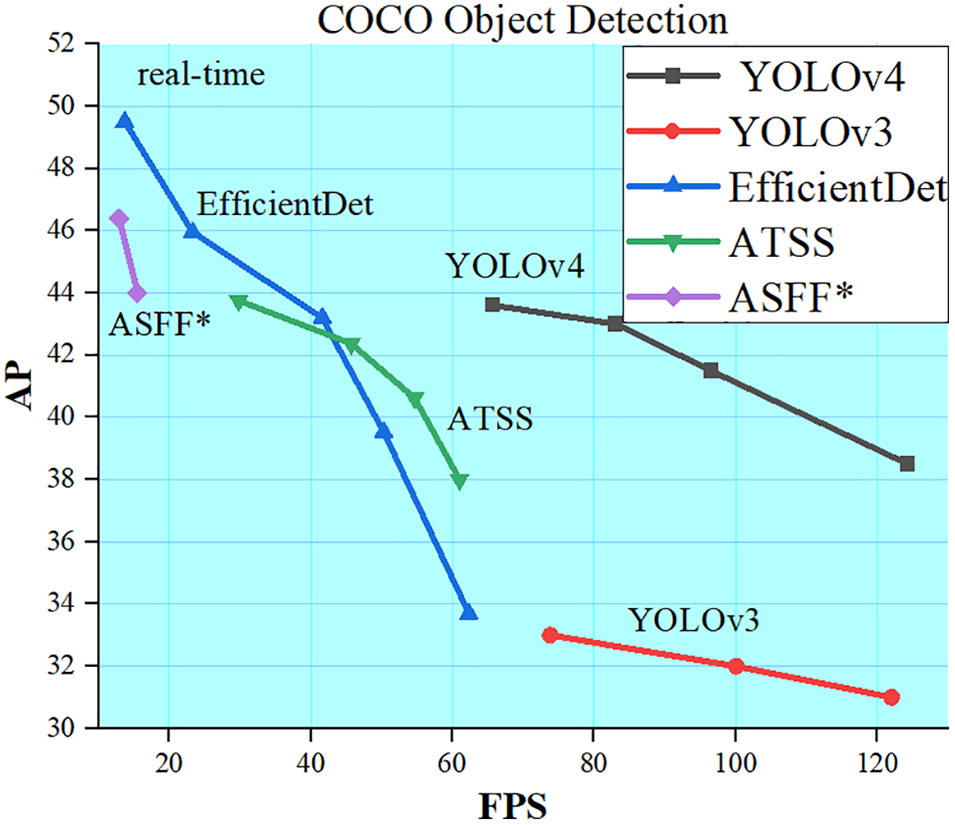
Figure 3: Performance comparison of target detection algorithms

3.2 Charge Port Image Acquisition

To obtain location information, image recognition and target detection algorithms need to be applied to the camera images, requiring real-time computing capability for the automatic charging system. The Jetson Nano addresses this need by running multiple neural networks simultaneously for various AI applications like object detection, speech processing, and image classification. Equipped with a quad-core CORTEX-A57 processor, a 128-core Maxwell GPU, and 4 GB of LPDDR RAM, the Jetson Nano delivers a powerful computing performance of 472GFLOPS and supports popular AI frameworks and algorithms.

The coordinates captured through the camera on the auto-charge are a rough value whose main function is to provide information on the general location of the charging port, which is used to guide the robotic arm joint to drive the charging gun to the nearby area. Since the camera used lacks depth information, it cannot obtain the distance between the charging gun and the plane where the charging port is located, so the coordinates cannot be determined directly, but the location of the charging port can be determined by the transformation relationship between the two pictures. The specific approach is to first human control the automatic charging device to achieve docking, and then control the charging robotic arm to exit along the direction of the central axis of the charging port to a certain distance d. Then the local camera is activated to take pictures and obtain the image in this state. During the photographing process, it is necessary to ensure that the image captured by the local camera at this distance contains the complete charging port.

3.3 Creation of the Charging Port Image Dataset

After capturing the image, the image needs to be processed, firstly extracting the location of the charging port in the image and segmenting its area to remove the interference of the background part. The YOLO algorithm is used in the step of determining whether the charging port exists or not. Based on the YOLOv4 network model, images of charging ports are collected, a dataset is created, and a model weight file specifically for identifying charging ports is trained by itself.

The step of segmenting the charge port region is called ROI extraction [22]. It is a selected region of the image outlined in boxes, circles, ellipses, irregular polygons, etc., from the image that is the focus of attention for image analysis and circling the region for further processing. Using ROI to circle a target reduces processing time, increases accuracy, and brings considerable convenience to image processing.

In this study, the rectangular box drawn by YOLOv4 in identifying the charging port is used. to locate the charging port, as shown in Fig. 4. And the original image is segmented by using the location size information of this rectangular box. Extracting the charging port region is for ROI extraction, as shown in Fig. 5.

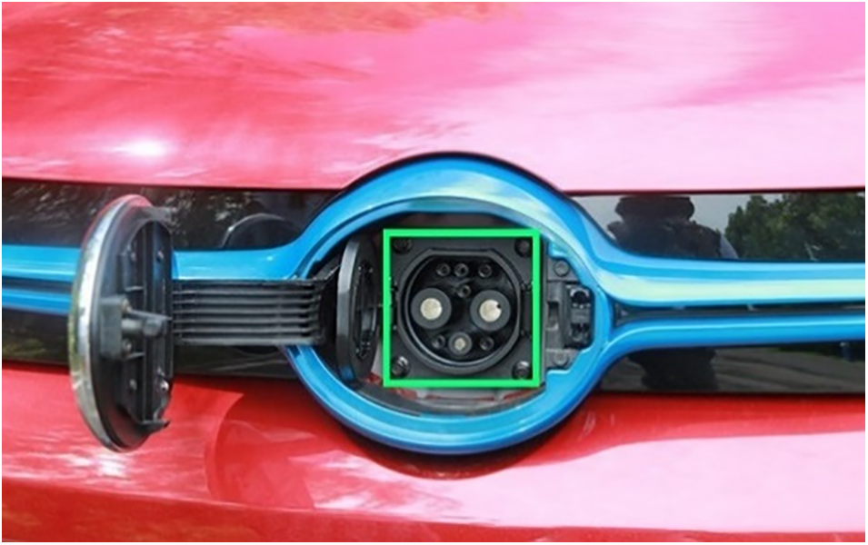
Figure 4: YOLO identification charging port

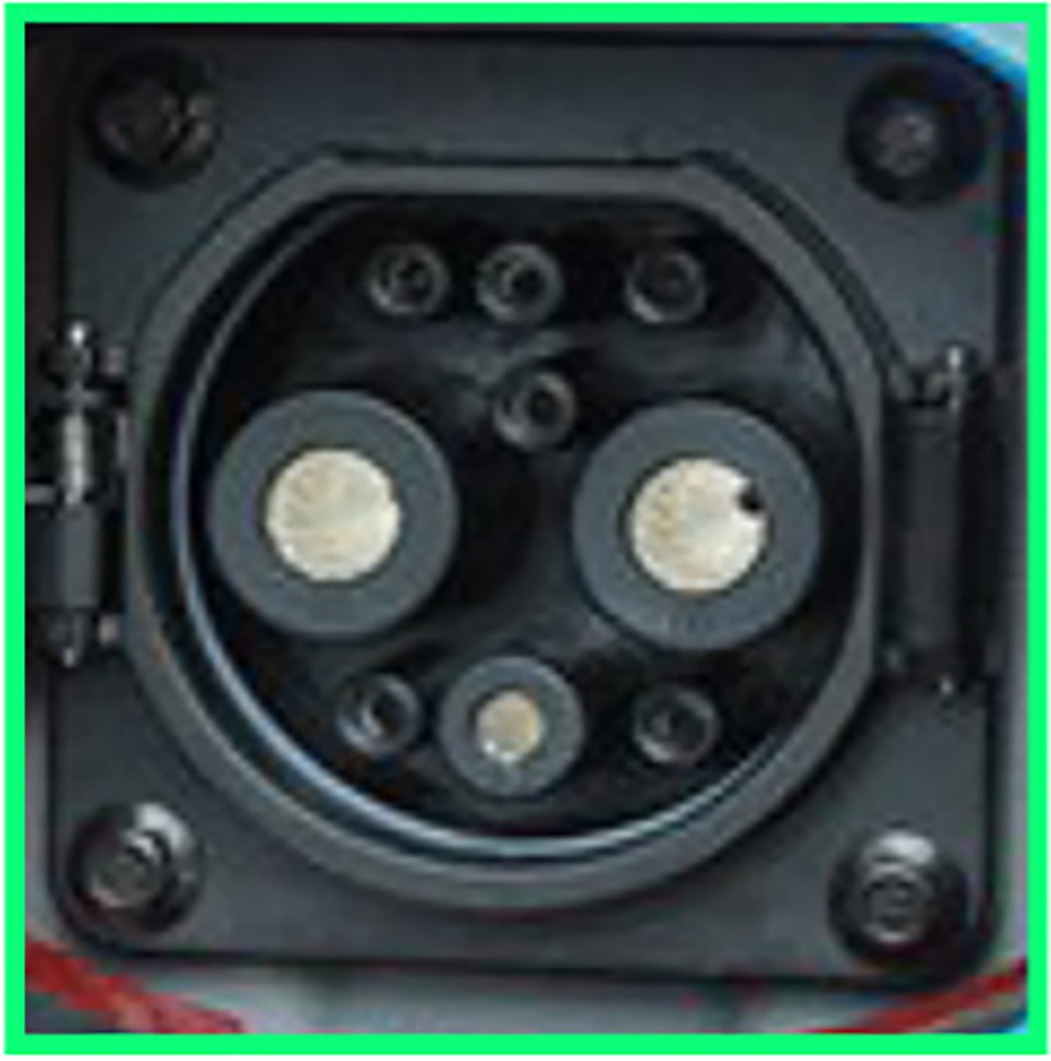
Figure 5: ROI extraction

To identify vehicles and charging ports, the YOLOv4 algorithm is employed, and approximately 1000 parking images are collected for each. This results in a total of 2000 images that comprise the dataset, as depicted in Fig. 6.

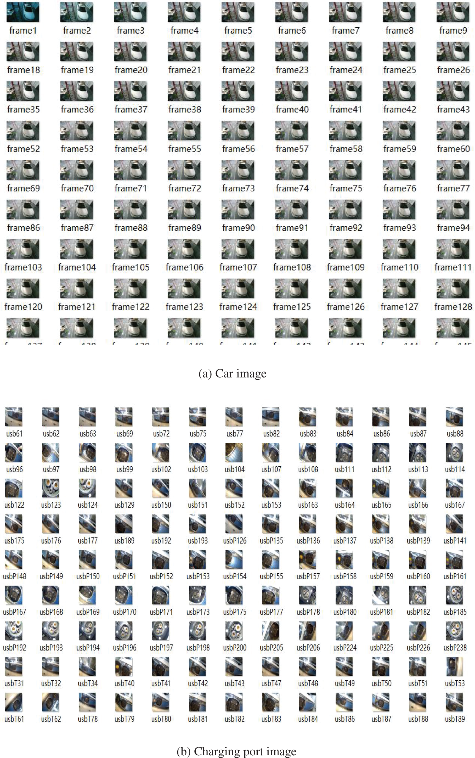
Figure 6: Vehicle image data set

3.4 Feature Point Detection Based on the Hough Circle Transform

The purpose of feature point detection is to obtain distinctive feature points of the charging port in the picture to be detected for matching localization, as shown in Fig. 7. As the fast charging port of the vehicle is a national standard, there is a fixed size and shape. The charging port consists of a typical cylindrical electrical connector; therefore, feature points are extracted from the charging port using Hough transform circle detection [23].

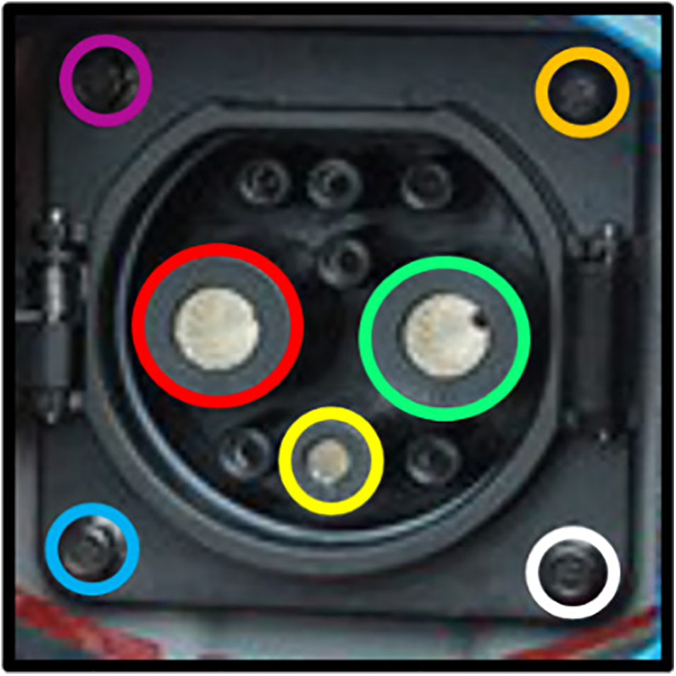
Figure 7: Hough transform circle detection and feature point extraction

3.5 Analysis of the Training Process for the Charging Port Dataset

A YOLOv4 convolutional neural network is trained using a sample set until the loss curves and evaluation indicators reach a stable state, and 100 iterations are performed. The training process is monitored by plotting the training set loss and learning rate curves in Fig. 8, and the charging port image data training set accuracy epoch graph in Fig. 9. The training effect is good as the loss rate and accuracy stabilize at 0.1 and 0.9, respectively, after 100 iterations.

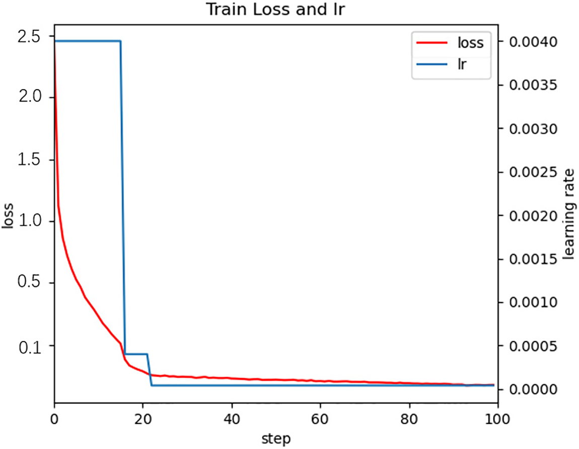
Figure 8: Training set loss plot and learning rate plot

Figure 9: Charging port image data training set accuracy epoch curve

Table 1 shows the performance comparison between YOLOv3 and YOLOv4 algorithms. With an unchanged training set and test set, YOLOv4 AP can reach 44, and the running speed is significantly improved.

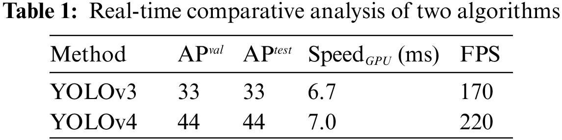
In this paper, the complexity of the target detection algorithm is calculated by the time complexity. To calculate the complexity of the YOLOv4 algorithm, it depends on the size of the input image, the depth of the network, and the hardware device. It takes about 14 s to process 2000 datasets.

3.6 Positioning of Charging Port Coordinates

In addition to deep learning to determine the specific location of the charge port coordinates, camera calibration is also required. Camera calibration refers to the relationship between the location of the camera image pixel points and the corresponding real environment point location. The calibration parameters mainly include internal and external parameters, where the internal parameter is the characteristic parameter of the camera itself. In contrast, the external parameter is the camera’s pose in the world coordinate system. The derivation of the formula leads to:

ZC[ uv1 ]=[ 1dx0u001dyv0001 ]  [ f0000f000010 ]  [ BM0→1 ]  [ XWYWZW1 ]=[ fx0u000fyv000010 ]  [ BM0→1 ]  [ XWYWZW1 ](1)

where K = [fx0u000fyv000011] is the internal reference of the camera and [BM0→1] is the external reference of the camera, both of which can be obtained by calibration. fxand fy are the focal lengths of the pixels in the x and y directions, respectively, and (u0, v0) is the pixel coordinate of the camera’s optical center.

From the Homography Matrix [24], denoted H, we know that a specific object in space, two pictures taken with a camera at different angles, image1 and image2, and there are P points in both pictures. The pixel coordinates of P points in the two pictures are P1 (u1, v1) and P2 (u2, v2), respectively. It can be simply considered that the transformation relationship between these two coordinates is the single-response transformation, i.e., P1 = HP2 (or P2 = HP1), written the homogeneous coordinates as:

K(B[XYZ]T+M)(2)

P = [X Y Z]T is a point in space, the picture taken by the camera at the initial position is image1, i.e., the positioning reference picture, at which point the movement of the camera has no rotation and no translation. is the unit matrix, is 0. P is a point in the picture, then the pixel coordinates P1 (u1, v1, 1) of point P in image1 satisfy:

s1P1=KP⇔P=s1K−1P1(3)

After the camera has moved with the rotation matrix R and translation matrix T, the picture is image2, which, to be detected, is taken and contains the spatial point P. The pixel coordinates P2 (u2, v2, 1) of the point P in image2 satisfy:

s2P2=K(BP+M)(4)

The point P is a point on the space plane, which is defined by:

nTP+d=0⇔−nTPd=1(5)

By combining Eqs. (3)–(5), we can get:

P2=s1s2K(B−nTMd)K−1P1(6)

H=s1s2K(B−nTMd)K−1(7)

Because of the scale invariance of homogeneous coordinates P1 and P2, s1, s2 are scale factors and their specific values are not considered, so the Homography Matrix H is:

H=K(B−nTMd)K−1(8)

In the charging port identification and positioning process, the shooting position of the positioning reference picture image1 is located directly in front of the vehicle charging port, as shown in Fig. 10, the center normal of the camera imaging plane (yellow dashed line in the figure) is parallel to the center axis of the charging port (red dashed line in the figure), the distance between the image plane and the charging port plane is d. At this time, the local camera position is recorded as Pcam1. The robotic arm only needs to be in this attitude. The robotic arm only needs to move in the direction parallel to the center axis of the charging port to complete the docking of the charging gun and the charging port.

Pcam1=[B1M101](9)

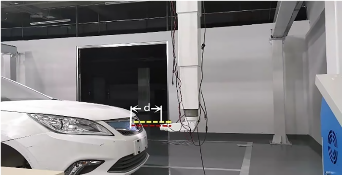
Figure 10: Diagram of the target image shooting position

The position of the picture to be detected varies depending on the result of the rough positioning, note that the local camera position at this point is Pcam2:

Pcam2=[B2M201](10)

The Homography Matrix formed by rotation matrix B and translation matrix M obtained by homologous matrix is:

Trans=[BM01](11)

The relationship among the three is as follows:

Pcam2⋅Trans=Pcam1(12)

The transformation of the coordinates of the same point P in space under the two camera coordinate systems Pcam1 and Pcam2 satisfies the relationship:

P2=B⋅P1+M(13)

However, it should be noted that B and M obtained from the Homography Matrix solution are quantities under the camera coordinate system relative to the Pcam1 local camera, without scale information, and cannot be directly superimposed and used when calculating the World coordinates of the point. The scale value between the two is the distance between the image plane and the charging port plane in Pcam1 as d. Therefore, the world coordinates of the point under the two camera coordinate systems satisfy the following relationship:

P2=B⋅P1+d⋅M(14)

4  Improving the RRT* Algorithm

4.1 RRT and the RRT* Algorithm

A diagram of the RRT expansion process is shown in Fig. 6. The principle is to take a starting point as the root node and generate a random expansion tree by sampling nodes randomly in a fast way. When all the nodes in the random tree enter the target region, a path from the starting point to the target point can be found. The random tree expansion process is shown in Fig. 11. L paths can be obtained by searching for the parent nodes from the target point until the starting point is reached. The one with the shortest length is selected as the final planned path.

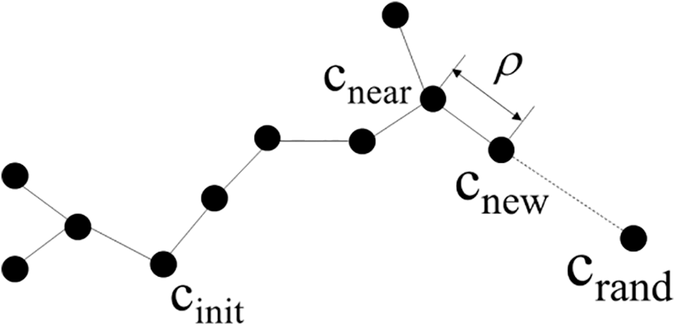
Figure 11: Diagram of the RRT extension process

The RRT algorithm is based on the following pseudo-code. The pseudo-code of the RRT algorithm is shown below:

The effectiveness and completeness of the RRT algorithm have been well verified, but the algorithm still suffers from low search efficiency, non-optimal paths, and excessive memory consumption.

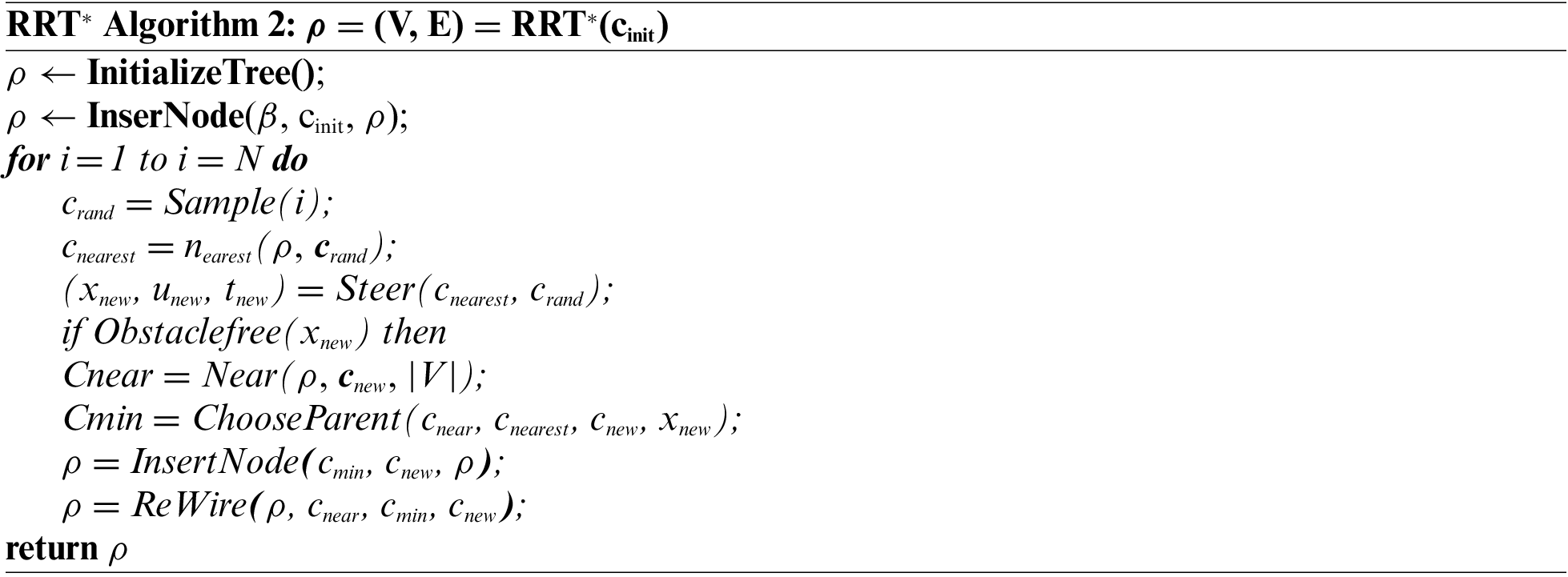
Therefore, some scholars have proposed the RRT* algorithm, which adds two new optimization-seeking processes, selecting the parent nodes and reconnecting them, when performing random tree expansion. In addition to adding the new node obtained by sampling to the tree, the algorithm also re-searches for the existence of a new parent node among the tree nodes contained within a circular neighborhood at a certain distance from the new node. If the new node is connected to that parent node to obtain a less costly path, the new node is reconnected to the parent node. The RRT* algorithm process is shown in Fig. 12. The pseudo code of the RRT* algorithm is shown below.

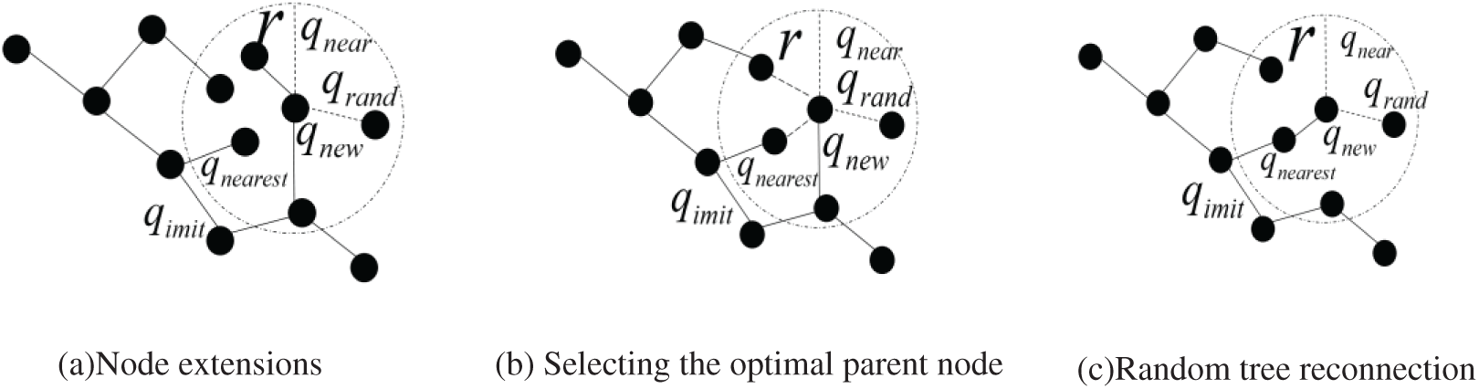
Figure 12: Path finding process of the RRT* algorithm

4.2 Principle of the Improved RRT* Algorithm

The traditional RRT* algorithm is asymptotically optimal, and its memory consumption and computational effort to prune the random tree T increases exponentially as the number of nodes continues to increase while the algorithm’s search efficiency and node usage continue to decrease.

An improved RRT* path planning algorithm for complex environments with multiple obstacles is proposed for the RRT algorithm memory consumption problem. The algorithm can improve the efficiency of the RRT* search and speed up the convergence speed, reducing memory consumption. The improved RRT* algorithm first simplifies the global raster map, based on which it finds the optimal set of path points from the starting point to the target point. The path is then used as a guide path for the algorithm. Then the guide path is expanded by an intelligent sampling factor to obtain an intelligent sampling region. And combine the un-simplified global raster map and the smart sampling area, and continuously iterate the search in the intelligent sampling area. A cost-effective, collision-free path from the starting point to the target point is obtained. Finally, combining the rotation radius of the automatic charging device and the B-sample curve-based path optimization, an optimized path with a smooth path and continuous curvature is generated. Thus, the mobile robot reaches the target point quickly, smoothly and safely along this globally optimized path.

For path optimization, the basic requirements must be met: continuity of the two-point trajectory, trajectory passing through a fixed point, and trajectory without collision. Each straight line is divided into small paths according to the nodes, and the time t for the robot arm to pass is assigned by the path length and the average speed, for which purpose, let P denote the trajectory path. Then the equation formed by P is:

p(t)=p0+p1t+p2t2⋯+pntn=∑i=0npiti(15)

p(t)=[1,t,t2,…,tn]⋅p(16)

v(t)=p′(t)=[0,1,2t,3t,4t2,…,ntn−1]⋅p(17)

a(t)=p″(t)=[0,0,2,6t,12t2,…,n(n−1)tn−2]⋅p(18)

jerk(t)=p(3)(t)=[0,0,0,6,24t,…,n!(n−3)!tn−3]⋅p(19)

snap(t)=p(4)(t)=[0,0,0,0,24,…,n!(n−4)!tn−4]⋅p(20)

pi=[pi0,pi1,…,pin]T(21)

p=[p1T,p2T,…,pkT]T(22)

Fig. 13 shows the improved RRT* algorithm flow.

Figure 13: Improved RRT* algorithm flow

5  Simulation Experiments and Analysis

Two experiments are designed to verify the improved RRT algorithm’s effectiveness. The first set of experiments does not consider the collision detection of the robotic arm, treats the robotic arm as a mass point in space, and conducts path planning simulation experiments on standard RRT, RRT* and improved RRT* in two-dimensional and three-dimensional space, respectively. In contrast, the second set of experiments builds an electric vehicle automatic charging model and completes the automatic charging of the vehicle through the algorithm.

5.1 Two-Dimensional Spatial Simulation

Set the simulation field (simulation field size 200 * 200), the geometry inside the box represents the obstacle, the area outside the geometry is the reachable area, and set the step size to 20. The maximum number of iterations is 3000. the MATLAB experimental platform is 2018b and 50 simulations are performed and the average value is taken. The thin short lines indicate the random tree branches, and the thick lines connecting the start and target points indicate the final generated paths. The simulation experiments ignore the robot’s own size and consider the environment after puffing. The same start point, end point and obstacles are designed when the environment is known. The comparison results of RRT, RRT*, other improved RRT* algorithms, and the improved RRT* algorithm in this paper are shown in the simulation experiments comparing the four algorithms in Fig. 14, Environment A, and Fig. 15, Environment B.

Figure 14: Comparison simulation experiment of four algorithms in Environment A

Figure 15: Comparison simulation experiment of four algorithms in Environment B

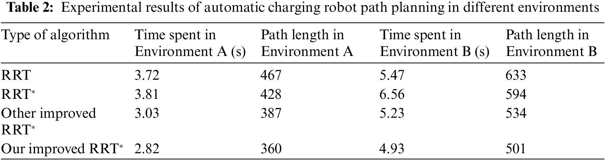
According to the experimental results in Table 2, it can be seen that in environment A, compared with the standard RRT, RRT* algorithm, and other improved RRT* algorithms, our improved RRT* algorithm consumes 24.2%, 26.0%, and 6.9% less time, and the path cost is the length of the whole path from the beginning to the end of the path, and the path cost is reduced by 22.9%, 15.9%, and 7.5%, respectively. In Environment B, our improved RRT* algorithm in this paper takes 10.1%, 24.8%, and 5.7% less time and the path cost is 20.9%, 15.7%, and 6.2% less, respectively.

5.2 Three-Dimensional Spatial Simulation

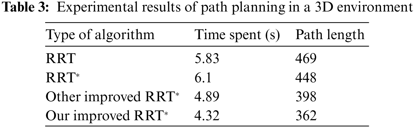
The size of the simulation map is 250 * 250 * 250; the starting point is (10, 10, 10), and the ending point is (200, 200, 200). And other parameters are kept the same as in the two-dimensional space experiment. The three-dimensional comparison results of RRT algorithm, RRT* algorithm, other improved RRT* algorithm and our improved RRT* algorithm are shown in Fig. 16. The comparison can be obtained: the improved RRT* algorithm in this paper reduces the invalid expansion of the random tree and the obtained paths are smoother. According to the experimental results in Table 3, it can be seen that compared with the standard RRT, RRT*, and other improved RRT* algorithms, our improved RRT algorithm takes 35.5%, 29.2%, and 11.7% less time, and the path length is reduced by 22.8%, 19.2%, and 9%, respectively. It shows that the improved RRT* algorithm in this paper has a good improvement in time and path length to meet the requirements.

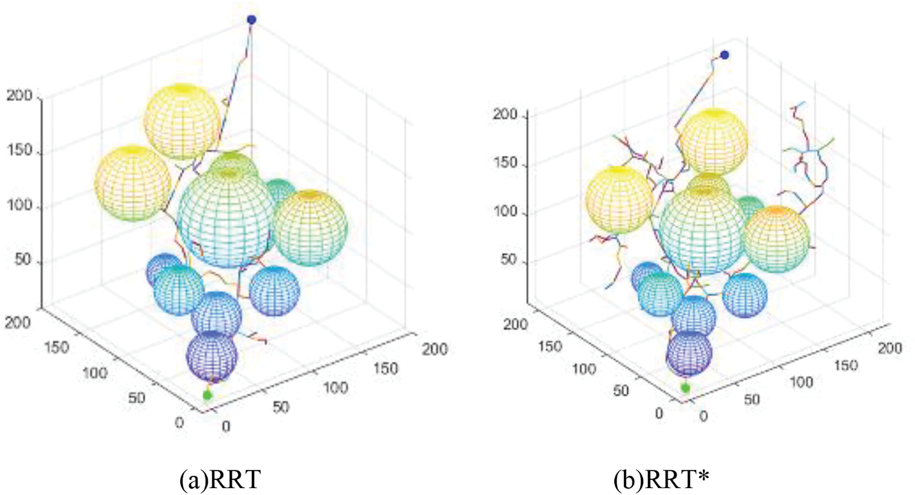
Figure 16: Simulation experiments comparing RRT with RRT* and RRT* in a 3D environment

6  Improved DH Method Modelling

6.1 Improved DH Coordinate System Establishment

The overall structure of the electric vehicle automatic charging robot arm is shown in Fig. 17. It is a 5-degree-of-freedom charging robot arm consisting of a moving truss, a telescopic robot arm, and a rotating joint. Theoretically, it can cover the cubic area of the truss and charge electric vehicles with charging ports arranged at different positions on the body. To simplify the difficulty of solving the positive and negative kinematics [25]. A modified DH coordinate system [26] is used for modeling, with the base coordinate system coinciding with the origin of coordinate system 1.

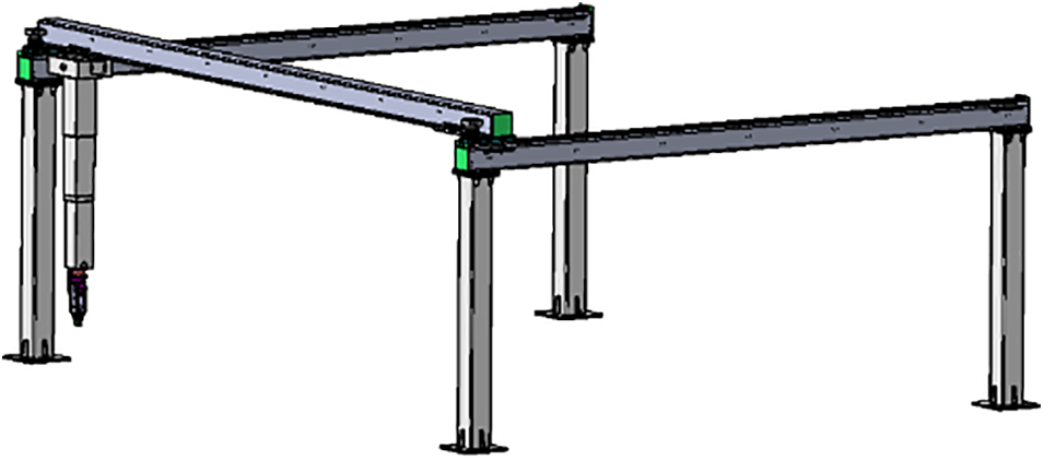
Figure 17: 3D model of the automatic charging robot arm

Based on the principle of establishing the D-H coordinate system, the truss charging robot arm is modeled with the modified DH coordinate system shown in Fig. 18.

Figure 18: Truss charging robot with improved DH coordinate system

6.2 Table of DH Parameters

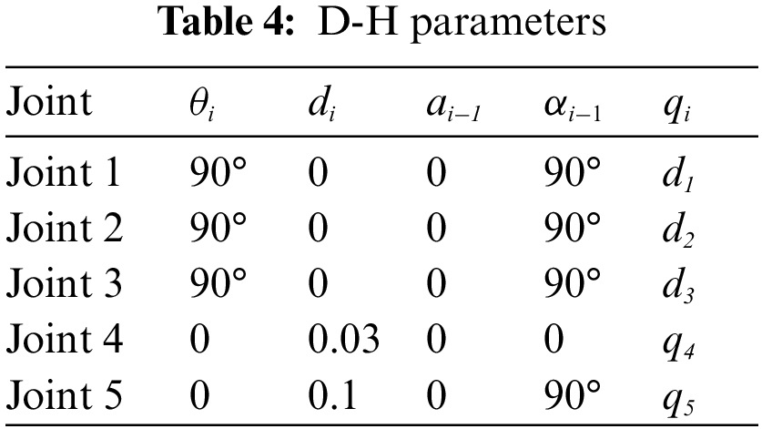
The standard D-H modeling of the truss auto-charging robot was carried out to obtain the D-H parameters of the kinematic model, θ, d, a, α, representing the joint rotation angle, linkage offset, linkage length, and linkage torsion angle, respectively. The D-H parameter table is thus generated and shown in Table 4.

6.3 Kinematic Solving

The joint angle is known, and the process of finding the spatial attitude and position of the end of the truss charging robot is the positive kinematic solution. The chi-square transformation matrix of two adjacent links is:

i−1Ti=TRX(αi−1)TX(ai−1)TRZ(qi)TZ(di)=[10000cαi−sαi00sαicαi00001][100ai010000110001][cqi−sqi00sqicqi0000100001][10000100001di0001]=[cqi−sqi0ai−1sqicαi−1cqicαi−1−sαi−1−sαi−1disqisαi−1cqisαi−1cαi−1cαi−1di0001](23)

The transformation matrix of two adjacent connecting rods can be derived from the above equation as follows:

0T1=[0100001d110000001]1T2=[0−10000−1−d210000001]2T3=[0100001d310000001]3T4=[cq4−sq400sq4cq4000010.030001]4T5=[cq5−sq50000−1−0.1sq5cq5000001](24)

The total flush transformation matrix at the actuating end of the truss charging robot can be introduced from the second transformation matrix of the two adjacent connecting rods with respect to the total flush transformation matrix based on the following:

0T5=0T11T22T33T44T5=[nxoxaxpxnyoyaypxnzozazpz0001](25)

where the equation for the end attitude of the auto-charging robot is:

nx=−cq4cq5ny=−cq5sq4n2=−sq5ox=cq4sq5oy=−sq4sq5oz=−cq5ax=−sq4ay=−cq4az=0(26)

6.4 Inverse Kinematic Solution

Based on the spatial location of the target position point, solve for the distance travelled by joint 1, joint 2 and joint 3:

0T1−1[nxoxaxpxnyoyaypxnzozazpz0001]=1T22T33T44T5(27)

By simplifying the above equation, we get:

[nzozazpznxoxaxpxnyoyaypy−d10001]=[−sq5−cq50−d3−0.03−cq4cq5cq4sq5−sq4d2−0.1sq4cq5sq4−sq4sq5−cq40.1cq40001](28)

From the above equation, we can see that:

d1=py−0.1cq4; d2=px+0.1sq4; d3=−pz−0.03(29)

Solve for the rotation angle of joint 4 and joint 5:

q4=arccos⁡(−ay),q5=arccos⁡(−oz)(30)

6.5 Work Area Analysis

The working space of a truss charging robot arm is the spatial range that the device can reach during normal operation, i.e., the maximum range in which the origin of the end joint coordinate system is active in space. The working space of the truss charging manipulator’s arm is denoted as W(P). Then the relationship between the amount of motion variation of the joint and the workspace can be expressed by the following equation:

W(P)={P(l),l∈Q}(31)

where W(P) denotes the working area of the truss robot arm; Q denotes the spatial constraint.

Fig. 19 shows that the robotic arm can span the entire cubic space, allowing each joint fit to reach any point in the working area. In the x-axis direction, the working range of the robotic arm is (0, 5.5); in the y-axis direction, the working range of the robotic arm is (0, 5.5); and in the z-axis direction, the working range of the robotic arm is (−1.8, 0) in unit m. According to the motion working domain, it is possible to better configuration of joint size for trajectory planning.

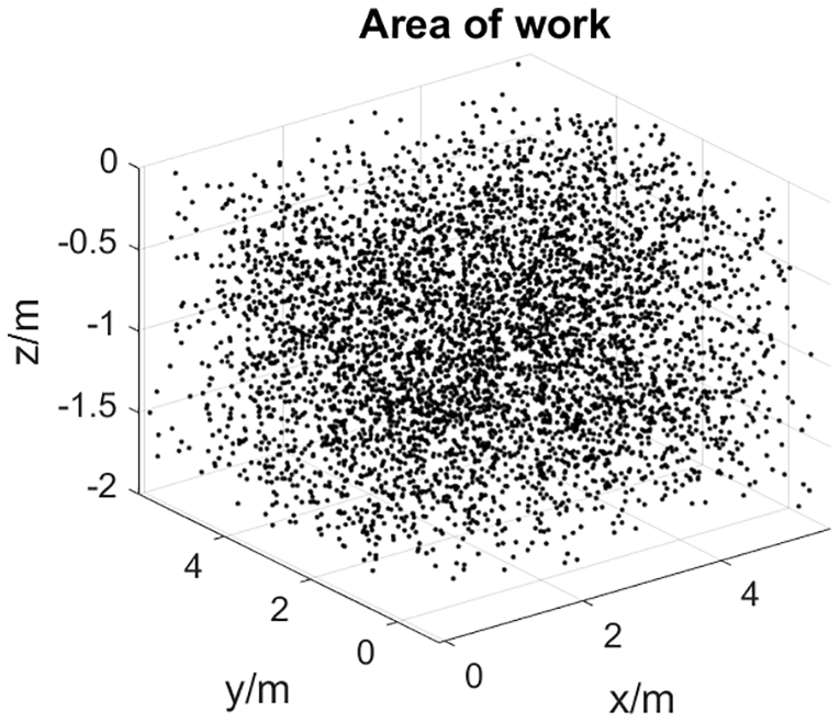
Figure 19: Automatic charging robot arm working area

7  Path Planning Experimental Simulation Analysis

Build an automatic charging robotic arm obstacle avoidance experimental platform, which consists of an automatic charging robotic arm, control box, electric vehicle, and PC side (CPU: Intel(R) Core(TM) i7-12700K @5.0 Ghz, GPU: NVIDIA GeForce GTX 2080Ti), etc. This paper uses the motion planning platform MoveIt! and the physical simulation platform Gazebo, two plug-in modules in ROS, to model and simulate the automatic charging device. The modeling and simulation environment used in this paper is Ubuntu 18.04, ROS melodic, MoveIt!

According to the built-in experimental platform, a virtual working platform is developed, as illustrated in Fig. 20, for the simulation of the motion of the automatic charging robot. The automatic charging robot arm is simplified to a tandem robot motion model with 3 degrees of freedom of movement and 2 degrees of freedom of rotation, as shown in Fig. 21. The effectiveness of the proposed algorithm is verified by comparing the improved RRT* with RRT* and the optimization data of the RRT algorithm in real and virtual experimental situations.

Figure 20: Experimental platform for automatic charging robot arm trajectory obstacle avoidance

Figure 21: Automatic charging device MoveIt! and Gazebo joint simulation

To verify the realism of the simulation results, the experimental verification is carried out by the experimental platform of the automatic charging robotic arm trajectory obstacle avoidance in Fig. 20 with a total of 20 experiments. The robot arm motion times of the improved RRT* algorithm were measured separately for 20 times. By comparing the motion times obtained experimentally with those optimized by the simulation, it can be seen. The range does not exceed 10%, as shown in Fig. 22. In turn, this shows the applicability of the improved RRT* algorithm to the automatic charging robot arm for obstacle avoidance.

Figure 22: Comparison of experimental and simulation time optimization results

8  Conclusion

The current research on the automatic charging of electric vehicles mainly focuses on industrial robotics, with little research on charging port identification and path planning. Therefore, it is crucial to study the recognition of charging ports for electric vehicles and the ability to achieve automatic charging robots that can avoid obstacles in complex environments after recognition. This paper presents an improved RRT* path planning algorithm based on a complex multi-obstacle environment. The algorithm can achieve fast search in the global range and search for optimal paths in complex environments. Then, through continuous iterative search, an asymptotically optimal and collision-free path is obtained from the starting point to the target point. Finally, the path optimization based on the B-sample curve generates a smooth and continuous curvature-optimized path so that the automatic charging robot arm can reach the endpoint smoothly and safely. Finally, the effectiveness and superiority of the algorithm in this paper are verified by comparing the simulation experiments of the improved RRT* algorithm with the RRT* algorithm and the RRT algorithm. In future research, we should further improve the accuracy of target detection and the speed and accuracy of the automatic charging robot in docking the charging port. The optimal path is found, and the arithmetic power is effectively reduced. In future research, algorithms that enable fast recognition, reconstruction and transformation of obstacles in dynamic environments are explored to reduce the time overhead of the process and combine the two in an attempt to better implement robotic arm obstacle avoidance planning for dynamic environments.

Funding Statement: This work was supported by National Natural Science Foundation of China (52175236).

Conflicts of Interest: The authors declare that they have no conflicts of interest to report regarding the present study.

References

1. Zhang, X., Gao, H., Guo, M., Li, G., Liu, Y. et al. (2016). A study on key technologies of unmanned driving. CAAI Transactions on Intelligence Technology, 1(1), 4–13. https://doi.org/10.1016/j.trit.2016.03.003 [Google Scholar] [CrossRef]

2. Zhou, X., Zhou, J. (2020). Data-driven driving state control for unmanned agricultural logistics vehicle. IEEE Access, 8, 65530–65543. https://doi.org/10.1109/ACCESS.2020.2983424 [Google Scholar] [CrossRef]

3. Meng, Y., Zhuang, H. (2007). Autonomous robot calibration using vision technology. Robotics and Computer-Integrated Manufacturing, 23(4), 436–446. https://doi.org/10.1016/j.rcim.2006.05.002 [Google Scholar] [CrossRef]

4. Dixit, S., Fallah, S., Montanaro, U., Dianati, M., Stevens, A. et al. (2018). Trajectory planning and tracking for autonomous overtaking: State-of-the-art and future prospects. Annual Reviews in Control, 45, 76–86. https://doi.org/10.1016/j.arcontrol.2018.02.001 [Google Scholar] [CrossRef]

5. Lim, W., Lee, S., Sunwoo, M., Jo, K. (2018). Hierarchical trajectory planning of an autonomous car based on the integration of a sampling and an optimization method. IEEE Transactions on Intelligent Transportation Systems, 19(2), 613–626. https://doi.org/10.1109/TITS.2017.2756099 [Google Scholar] [CrossRef]

6. Ohnishi, K., Matsui, N., Hori, Y. (1994). Estimation, identification, and sensorless control in motion control system. Proceedings of the IEEE, 82(8), 1253–1265. https://doi.org/10.1109/5.301687 [Google Scholar] [CrossRef]

7. Han, D., Nie, H., Chen, J., Chen, M. (2018). Dynamic obstacle avoidance for manipulators using distance calculation and discrete detection. Robotics and Computer-Integrated Manufacturing, 49, 98–104. https://doi.org/10.1016/j.rcim.2017.05.013 [Google Scholar] [CrossRef]

8. Hentout, A., Maoudj, A., Aouache, M. (2022). A review of the literature on fuzzy-logic approaches for collision-free path planning of manipulator robots. Artificial Intelligence Review, 1–76. https://doi.org/10.1007/s10462-022-10257-7 [Google Scholar] [CrossRef]

9. Huang, Y., Abu-Dakka F. J., Silvério, J., Caldwell D. G. (2020). Toward orientation learning and adaptation in cartesian space. IEEE Transactions on Robotics, 37(1), 82–98. https://doi.org/10.1109/TRO.2020.3010633 [Google Scholar] [CrossRef]

10. Wang, W., Zhu, M., Wang, X., He, S., He, J. et al. (2018). An improved artificial potential field method of trajectory planning and obstacle avoidance for redundant manipulators. International Journal of Advanced Robotic Systems, 15(5), 1729881418799562. https://doi.org/10.1177/1729881418799562 [Google Scholar] [CrossRef]

11. Miao, C., Chen, G., Yan, C., Wu, Y. (2021). Path planning optimization of indoor mobile robot based on adaptive ant colony algorithm. Computers & Industrial Engineering, 156, 107230. https://doi.org/10.1016/j.cie.2021.107230 [Google Scholar] [CrossRef]

12. Zhou, X., Ma, H., Gu, J., Chen, H., Deng, W. (2022). Parameter adaptation-based ant colony optimization with dynamic hybrid mechanism. Engineering Applications of Artificial Intelligence, 114, 105139. https://doi.org/10.1016/j.engappai.2022.105139 [Google Scholar] [CrossRef]

13. Blum, C. (2005). Ant colony optimization: Introduction and recent trends. Physics of Life Reviews, 2(4), 353–373. https://doi.org/10.1016/j.plrev.2005.10.001 [Google Scholar] [CrossRef]

14. Zhang, L., Lin, Z., Wang, J., He, B. (2020). Rapidly-exploring random trees multi-robot map exploration under optimization framework. Robotics and Autonomous Systems, 131, 103565. https://doi.org/10.1016/j.robot.2020.103565 [Google Scholar] [CrossRef]

15. Salzman, O., Halperin, D. (2016). Asymptotically near-optimal RRT for fast, high-quality motion planning. IEEE Transactions on Robotics, 32(3), 473–483. https://doi.org/10.1109/TRO.2016.2539377 [Google Scholar] [CrossRef]

16. Jeong, I. B., Lee, S. J., Kim, J. H. (2019). Quick-RRT*: Triangular inequality-based implementation of RRT* with improved initial solution and convergence rate. Expert Systems with Applications, 123, 82–90. https://doi.org/10.1016/j.eswa.2019.01.032 [Google Scholar] [CrossRef]

17. Wang, J., Li, B., Meng M, Q. H. (2021). Kinematic constrained Bi-directional RRT with efficient branch pruning for robot path planning. Expert Systems with Applications, 170, 114541. https://doi.org/10.1016/j.eswa.2020.114541 [Google Scholar] [CrossRef]

18. Yuan, C., Liu, G., Zhang, W., Pan, X. (2020). An efficient RRT cache method in dynamic environments for path planning. Robotics and Autonomous Systems, 131, 103595. https://doi.org/10.1016/j.robot.2020.103595 [Google Scholar] [CrossRef]

19. Li, D., Du, L. (2022). Recent advances of deep learning algorithms for aquacultural machine vision systems with emphasis on fish. Artificial Intelligence Review, 55(5), 4077–4116. https://doi.org/10.1007/s10462-021-10102-3 [Google Scholar] [CrossRef]

20. Zhu, H., Sun, C., Zheng, Q., Zhao, Q. (2023). Deep learning based automatic charging identification and positioning method for electric vehicle. Computer Modeling in Engineering & Sciences, 136(3), 3265–3283. https://doi.org/10.32604/cmes.2023.025777 [Google Scholar] [CrossRef]

21. Bochkovskiy, A., Wang, C. Y., Liao, H. Y. M. (2020). YOLOv4: Optimal speed and accuracy of object detection. arXiv preprint arXiv:2004.10934. [Google Scholar]

22. Singh, J., Arora A, S. (2020). Automated approaches for ROIs extraction in medical thermography: A review and future directions. Multimedia Tools and Applications, 79(21), 15273–15296. https://doi.org/10.1007/s11042-018-7113-z [Google Scholar] [CrossRef]

23. Yuen, H., Princen, J., Illingworth, J., Kittler, J. (1990). Comparative study of Hough transform methods for circle finding. Image and Vision Computing, 8(1), 71–77. https://doi.org/10.1016/0262-8856(90)90059-E [Google Scholar] [CrossRef]

24. Fan, R., Wang, H., Cai, P., Wu, J., Bocus M, J. et al. (2021). Learning collision-free space detection from stereo images: Homography matrix brings better data augmentation. IEEE/ASME Transactions on Mechatronics, 27(1), 225–233. https://doi.org/10.1109/TMECH.2021.3061077 [Google Scholar] [CrossRef]

25. Ye, H., Wang, D., Wu, J., Yue, Y., Zhou, Y. (2020). Forward and inverse kinematics of a 5-DOF hybrid robot for composite material machining. Robotics and Computer-Integrated Manufacturing, 65, 101961. https://doi.org/10.1016/j.rcim.2020.101961 [Google Scholar] [CrossRef]

26. Tian, B. Q., Yu, J. C., Zhang, A. Q. (2015). Dynamic modeling of wave driven unmanned surface vehicle in longitudinal profile based on DH approach. Journal of Central South University, 22(12), 4578–4584. https://doi.org/10.1007/s11771-015-3008-6 [Google Scholar] [CrossRef]