Reliability Analysis of HEE Parameters via Progressive Type-II Censoring with Applications

1  Introduction

Modelling actual data using generalized distributions is still important today. A variety of generalized distributions have been developed, and their usefulness in various contexts is investigated, see for example the work of Nadarajah et al. [1] and Mahdavi et al. [2]. By combining the exponential and Harris distributions, Pinho et al. [3] created a new three-parameter lifetime model known as the Harris extended-exponential (HEE) distribution. They emphasized that the HEE distribution can be utilized as a substitute of the Weibull and gamma distributions for modelling data with a rising or decreasing failure rate. As a result, it can be applied in a variety of domains, including but not limited to reliability, biology, engineering, insurance and epidemiology, among others.

However, if X is a random variable that follows the HEE distribution, denoted by X∼HEE(Ψ), where Ψ=(α,β,θ)⊤ is the parameters vector with scale parameter β and shape parameters α and θ, then its probability density function (PDF) and cumulative distribution function (CDF) can be written, respectively, as

f(x;Ψ)=βθ1αe−βx[1−θ¯e−αβx]1+1α,x>0,α,β,θ>0,(1)

and

F(x;Ψ)=1−[θe−αβx1−θ¯e−αβx]1α,(2)

where θ¯=1−θ. One can see that when α=1, the HEE distribution reduces to the Marshall–Olkin exponential distribution proposed by Marshall et al. [4]. Also, the exponential distribution can be obtained as a special case from the HEE distribution by putting α=θ=1. The associated reliability characteristics of X such as reliability function (RF) and hazard rate function (HRF), at mission time t, are expressed, respectively, as follows:

R(t;Ψ)=[θe−αβt1−θ¯e−αβt]1α(3)

and

h(t;Ψ)=β[1−θ¯e−αβt]−1.(4)

Fig. 1a displays different plots of the PDF using various choices of parameters. Similarly, Fig. 1b shows the plots of the HRF. Fig. 1a indicates that the PDF of the HEE distribution can be decreasing or unimodal. On the other hand, its HRF allows for decreasing and increasing shape hazard rates.

Figure 1: Shapes of the PDF and HRF of the HEE distribution

In reliability analysis and life testing studies, the examined items are commonly lost or discarded before failure. The obtained sample is therefore known as a censored sample. To preserve the functional experimental units for future use, shortening the duration of the test, and saving money are some major justifications for removing the experimental units. Various censoring techniques, such as time and failure censoring, are available in the literature; nevertheless, they do not have the ability to permit units to be eliminated at any moment other than the experiment’s endpoint. As a result, a more flexible censoring scheme known as progressive Type-II censoring is offered. For more in-depth analysis, or to be used as test samples in other research, certain items may need to be removed from the experiment.

The schematic representation of the progressive Type-II censoring scheme is as follows: Assume that m units will fail out of n distinct units that are put on a life test. Allow (R1,R2,…,Rm) to be fixed in advance such that when the first failure occurs, X1:m:n, R1 units are arbitrarily removed from the experiment. When the experiment has its second failure, X2:m:n, R2 units from the remaining items are at random deleted from the test, and so on. When the mth failure Xm:m:n occurred, all Rm remaining items are extracted from the test. It is clear that n=m+∑i=1mRi. When Ri=0,i=1,…,m−1 and Rm=n−m, the case of conventional Type-II censored sampling arises. The progressive Type II censoring plan reduces to the case of a complete sample when Ri=0,i=1,…,m. If we assume that a continuous population with CDF F(⋅), and PDF f(⋅), then the likelihood function for a progressively Type-II censored sample can be expressed as below:

L(Ψ)=C∏i=1mf(xi:m:n)[1−F(xi:m:n)]Ri,(5)

where C=n(n−R1−1)…(n−∑i=1m−1(1+Ri)). Many studies used progressively Type-II censored data to consider some estimation issues for various lifetime distributions.

In literature, different censoring schemes were introduced; however, authors prefer to deal with progressive censoring over other censoring plans because it allows survival items to be withdrawn during the experiment at different stages which is not possible in case of failure (Type-II) censoring. Sultan et al. [5] investigated the classical and Bayesian estimation of inverse Weibull distribution. Dey et al. [6] investigated the maximum likelihood and Bayesian estimations for Marshall–Olkin extended exponential distribution. Kotb et al. [7] studied the inferences for modified Weibull distribution. Bdair et al. [8] analyzed the estimation and prediction for flexible Weibull distribution. Wu et al. [9] discussed the estimation and prediction problems for the Nadarajah–Haghighi parameters. Alotaibi et al. [10] considered the estimation of some reliability indices for alpha power Weibull distribution. Elshahhat et al. [11] considered the Bayesian life analysis of generalized Chen’s parameters. Dey et al. [12] studied various inferences for the Wilson–Hilferty parameters. For additional details regarding the concept of progressive censoring, one can guide Balakrishnan et al. [13].

Despite the flexibility and adaptability of the HEE distribution in modelling different types of data, to the best of our knowledge, there is no existing study on censoring mechanisms that deals with the estimation of parameters and/or reliability characteristics of the HEE distribution under incomplete (censored) sampling, which is of great interest and practical importance in many real-world scenarios. So, this study stands out in that it is the first to investigate the estimation issues for the HEE distribution when using incomplete data collected from a progressively Type-II censoring. Consequently, the main purposes for this study are fourfold:

•   First objective explores various point and interval estimation issues of the HEE distribution parameters as well as its reliability characteristics utilizing progressive Type-II censored data, namely: maximum likelihood estimators (MLEs), Bayes estimators, approximate confidence intervals (ACIs) and highest posterior density (HPD) credible intervals.

•   In Bayesian analysis, utilizing Markov Chain Monte Carlo (MCMC) techniques, the estimators are acquired by employing the squared-error (SE) and general entropy (GE) loss functions.

•   The second objective performs extensive Monte Carlo simulations to compare the performance of the proposed estimation methods on the basis of their simulated root mean squared errors, mean absolute biases, average confidence lengths and coverage probabilities.

•   The third objective is to check various optimality criteria to decide the best progressive censoring schemes.

•   The last one is to demonstrate the ability of the proposed methods to work in practice by exploring two actual real data sets.

Before going any further, it is important to remember that the limitations of this study are: (i) All inferential methodologies are developed based on the assumption that at least one survival item was removed during the life-test; (ii) We assumed that the HEE parameters α, β and θ as well as its related parametric functions R(t) and h(t) are unknown.

The remaining sections of the study are organized as follows: Section 2 presents MLEs and ACIs. Section 3 investigates the Bayes estimators and HPD credible intervals. The results of the simulation study are included in Section 4. We offer several ways to select the optimum censoring scheme in Section 5. Section 6 highlights the analysis of two real data applications. The paper is finally concluded in Section 7.

2  Likelihood Inference

In this section, the MLEs of the unknown parameters including the RF and HRF of the HEE distribution are investigated. Moreover, the ACIs based on the asymptotic properties of the MLEs are constructed. Assume that x_=(x1,…,xm), where xi=xi:m:n,i=1,…,m, for simplicity, be a progressively Type-II censored sample selected from a population with PDF and CDF given by (1) and (2), respectively. Given a predetermined progressive censoring scheme R1,…,Rm, then the likelihood function, without the constant term, can be derived from (1), (2) and (5) as follows:

L(Ψ|x_)=βmθnαe−β∑i=1mRi∗xi∏i=1m[1−θ¯e−αβxi]−(1+α¯Ri∗),(6)

where Ri∗=1+Ri and α¯=1/α. Instead of maximizing the likelihood function in (6), it is more convenient to work with its natural logarithm. Thus, it follows:

ℓ(Ψ|x_)=mlog⁡(β)+nαlog⁡(θ)−β∑i=1mRi∗xi−∑i=1m(1+α¯Ri∗)log⁡[1−θ¯e−αβxi],(7)

where ℓ(Ψ|x_)=log⁡L(Ψ|x_). The MLEs of α,β and θ, denoted by α^,β^ and θ^, are obtained by maximizing (7) with respect to α,β and θ. An equivalent way to obtain the MLEs is to solve the three normal equations simultaneously, which are acquired by getting the first order derivatives of the objective function in (7) with respect to the unknown parameters and equating the result by zero. Consequently, the normal equations are

∂ℓ(Ψ|x_)∂α=−nlog⁡(β)α2+1α2∑i=1mRi∗log⁡[1−θ¯vi]−βθ¯∑i=1m(1+α¯Ri∗)xivi1−θ¯vi=0,(8)

∂ℓ(Ψ|x_)∂β=mβ−∑i=1mRi∗xi−αθ¯∑i=1m(1+α¯Ri∗)xivi1−θ¯vi=0(9)

and

∂ℓ(Ψ|x_)∂θ=nαθ−∑i=1m(1+α¯Ri∗)vi1−θ¯vi=0,(10)

where vi=e−αβxi. It is clear from (8)–(10), that the MLEs α^, β^ and θ^ have no closed forms. Therefore, numerical methods may be implemented to solve these equations to produce α^,β^ and θ^. Since the MLE of α, β or θ cannot be solved analytically, the ‘maxLik’ package (which implements the Newton–Raphson (NR) method of maximization) proposed by Henningsen et al. [14] can be easily used. On the other hand, instead of NR method, the expectation–maximization (EM) or stochastic EM algorithm can be easily incorporated. For details, see Panahi [15,16].

Once the MLEs of α,β and θ are obtained, we can get the MLEs of R(t) and h(t) by using the invariance property of the MLEs as follows:

R^(t)=[θ^e−α^β^t1−θ¯^e−α^β^t]1α^,andh^(t)=β^[1−θ¯^e−α^β^t]−1,

where θ¯^=1−θ^.

After getting the point estimates of α,β and θ as well as the reliability indices, it is also of appeal to construct the associated confidence intervals. This objective can be achieved by employing the asymptotic properties of the MLEs. It is known that based on the theory of large samples that the asymptotic distribution of Ψ^, where Ψ^=(α^,β^,θ^)⊤, is normal distribution with average Ψ^ and variance-covariance matrix I3×3−1(Ψ) which is obtained by taking the inverse of the Fisher information (FI) matrix. It is not easy to obtain the elements of the FI matrix due to its intractable elements. Therefore, we can use the observed FI matrix to obtain I3×3−1(Ψ^) as an estimate of I3×3−1(Ψ), where

I3×3−1(Ψ^)=[−Fαα−Fαβ−Fαθ−Fβα−Fββ−Fβθ−Fθα−Fθβ−Fθθ](α,β,θ)=(α^,β^,θ^)−1=[σ^αασ^αβσ^αθσ^ββσ^βθσ^θθ],(11)

where the main diagonal elements are the estimated variances of α^,β^ and θ^, respectively, and the elements of the observed FI matrix can be easily obtained from (7) as follows:

∂2ℓ(Ψ|x_)∂α2=2nlog⁡(θ)α2−2α3∑i=1mRi∗log⁡[1−θ¯vi]+βθ¯∑i=1mxivi1−θ¯vi[2Ri∗α2+βxi(1+α¯Ri∗)1−θ¯vi],

∂2ℓ(Ψ|x_)∂β2=−mβ2+θ¯α2∑i=1m(1+α¯Ri∗)vixi2(1−θ¯vi)2,

∂2ℓ(Ψ|x_)∂θ2=−nαθ2+∑i=1m(1+α¯Ri∗)vi2(1−θ¯vi)2,

∂2ℓ(Ψ|x_)∂α∂β=−θ¯∑i=1mxivi1−θ¯vi+θ¯αβ∑i=1m(1+α¯Ri∗)vixi2(1−θ¯vi)2,

∂2ℓ(Ψ|x_)∂α∂θ=−nαθ2+1α2∑i=1mRi∗vi1−θ¯vi+β∑i=1m(1+α¯Ri∗)xivi1−θ¯vi[1+θ¯vi1−θ¯vi]

and

∂2ℓ(Ψ|x_)∂β∂θ=α∑i=1m(1+α¯Ri∗)xivi(1−θ¯vi)2.

Now, the 100(1−γ)% ACIs of α,β and θ can be acquired as follows:

α^±zγ/2σαα,β^±zγ/2σββandθ^±zγ/2σθθ,

where zγ/2 is the upper (γ/2)th percentile point of the standard normal distribution.

On the other hand, the ACIs of the RF and HRF can be also obtained by approximating the variances of their estimators by using the delta method. See Greene [17] for more details about the delta method. In this case, we can approximate the variances of R^(t) and h^(t) by σ^R=DRI3×3−1(Ψ^)DR⊤ and σ^h=DhI3×3−1(Ψ^)Dh⊤, respectively, where

DR=(∂R(t)∂α,∂R(t)∂β,∂R(t)∂θ)|(α,β,θ)=(α^,β^,θ^)

and

Dh=(∂h(t)∂α,∂h(t)∂β,∂h(t)∂θ)|(α,β,θ)=(α^,β^,θ^),

with the following elements

∂R(t)∂α=−1α2(θvt1−θ¯vt)1α[log⁡(θvt1−θ¯vt)+αβt1−θ¯vt],

∂R(t)∂β=−(1−θ¯vt)−1(θvt1−θ¯vt)1α,∂R(t)∂θ=vt−1αθ(1−θ¯vt)(θtαvt1−θ¯vt,)1α

∂h(t)∂α=−tθ¯β2vt(1−θ¯vt)2,∂h(t)∂β=1−θ¯vt(1+βαt)(1−θ¯vt)2,and∂h(t)∂θ=−βvt(1−θ¯vt)2,

where vt=e−αβt. Based on the above results, the ACIs for RF and HRF at the confidence level 100(1−γ)% can be expressed, respectively, as

R^±zγ2σ^Randh^±zγ2σ^h.

Though the main problem of ACI for a positive parameter is that it may give a negative value in the lower bound. In literature, there are different approaches available to handle this problem. Theoretically, one of them is called the log-transformed maximum likelihood estimator developed by Meeker et al. [18]. Numerically, one can easily verify that the computed confidence intervals contain a lower bound with a positive value if one of them contains a negative lower bound, in which case this value is replaced by zero. Recently, this issue has been examined by Elshahhat et al. [11] and Elshahhat et al. [19].

3  Bayes MCMC Inference

In this section, we consider the Bayesian estimation method to derive the Bayesian estimators for α,β and θ, as well as the R(t) and h(t). Besides the point estimates, we also acquire the HPD credible intervals for the different parameters. In statistical analysis, the Bayesian method has significant advantages over the classical methods when data availability is a critical barrier. In Bayesian inference, prior distribution selection is important. Since the gamma density prior, based on its parameter values, provides various shapes, see Dey et al. [20]. Thus, it is flexible and can be adopted as a suitable prior for the HEE parameters. Therefore, we utilize the Bayesian estimation under the assumption that the unknown model parameters α,β and θ are independent and follow gamma (G) distributions, i.e., α∼G(a1,b1), β∼G(a2,b2) and θ∼G(a3,b3), where ak and bk,k=1,2,3, are the hyper-parameters and are always positive. Using these premises, we can simply write the joint prior distribution of α,β and θ in the following form:

g(Ψ)∝αa1−1βa2−1θa3−1e−(b1α+b2β+b3θ).(12)

To get the Bayes estimates, we should first derive the joint posterior distribution of the unknown parameters. To obtain the joint posterior distribution, we combine the sample information given by (6) with the prior information about the unknown parameters given by (12) and apply the Bayes theorem. As a result, we can write the joint posterior distribution as follows:

π(Ψ|x_)=A−1αa1−1βm+a2−1θnα+a3−1e−β(∑i=1mRi∗xi+b2)−(b1α+b3θ)∏i=1m[1−θ¯e−αβxi]−(1+α¯Ri∗),(13)

where A is the normalized constant and obtained as

A=∫0∞∫0∞∫0∞αa1−1βm+a2−1θnα+a3−1e−β(∑i=1mRi∗xi+b2)−(b1α+b3θ)∏i=1m[1−θ¯e−αβxi]−(1+α¯Ri∗)dαdβdθ.

The loss function is crucial to Bayesian analysis because it may be used to characterize overestimation and underestimation in the investigation. Symmetric and asymmetric loss are two often employed loss functions. While the asymmetric loss function offers various weights to overestimation and underestimation, the symmetric loss function treats overestimation and underestimation equally. The asymmetric loss is more practical and advantageous in real-world applications than the symmetric loss see for more details Nassar et al. [21]. One of the most popular symmetric loss functions is the SE loss function, whereas the GE loss function is asymmetric. The SE and GE loss functions are considered in this work to acquire the Bayes estimates. It is generally known that the posterior mean is the Bayes estimator in the case of the SE loss function. On the other hand, the GE loss function provides varying weights for overestimation and underestimation.

Let μ~ is an estimator of μ, then according to Calabria et al. [22], the GE loss function can be expressed as

E(μ~,μ)∝(μ~/μ)δ−δlog⁡(μ/μ)−1,δ≠0,

where δ determines the degree of asymmetry. In this case, the Bayes estimator of δ can be obtained as

μ~GE=[Eμ(μ−δ)]−1δ,(14)

given that Eμ(μ−δ) exists and is finite. Assume that Φ(Ψ) be any function of the unknown parameters. Therefore, the Bayes estimators of Φ(Ψ) based on SE and GE loss functions can be obtained, respectively, as

Φ~SE(Ψ)=∫0∞∫0∞∫0∞Φ(Ψ)π(Ψ|x_)dαdβdθ(15)

and

Φ~GE(Ψ)=[∫0∞∫0∞∫0∞[Φ(Ψ)]−δπ(Ψ|x_)dαdβdθ]−1δ,(16)

where π(Ψ|x_) is the joint posterior distribution given by (13). It is obvious that it is impossible to calculate the Bayes estimators using (15) and (16) analytically due to the complex forms of the integration. In order to acquire the Bayes estimates of the unknown parameters and the corresponding HPD credible intervals in this case, we suggest using the MCMC technique. We first must establish the full conditional distributions of α,β and θ before we can use the MCMC approach. Given (13), the necessary full conditional distributions can be determined as below:

π(α|β,θ,x_)∝αa1−1θnαe−b1α∏i=1m[1−θ¯e−αβxi]−(1+α¯Ri∗),(17)

π(β|α,θ,x_)∝βm+a2−1e−β(∑i=1mRi∗xi+b2)∏i=1m[1−θ¯e−αβxi]−(1+α¯Ri∗)(18)

and

π(θ|α,β,x_)∝θnα+a3−1e−b3θ∏i=1m[1−θ¯e−αβxi]−(1+α¯Ri∗).(19)

Even though we have the full conditional distributions for each parameter, they do not have a known form, making it difficult to directly take samples from them. Therefore, we utilize the Metropolis–Hasting (M–H) algorithm to generate samples from these distributions. In order to derive the Bayesian estimates and the HPD credible intervals, we assume the normal distribution as the proposal distribution for the M–H sampling. Using the full conditional distributions given by (17)–(19), the required steps for the MH algorithm are as below

Step 1. Start with p=1.

Step 2. Determine the beginning values such that (α(0),β(0),θ(0))=(α^,β^,θ^).

Step 3. Generate α(p) from (17) using the M-H steps and N(α(p−1),σ^αα).

Step 4. From (18) and (19), generate β(p) and θ(p), respectively, by repeating Step 3.

Step 5. Use the generated sample (α(p),β(p),θ(p)) to obtain R(p)(t) and h(p)(t) from (3) and (4), respectively.

Step 6. Put p=p+1.

Step 7. Replicate Steps 3–6, N times to get α(p),β(p),θ(p),R(p)(t) and h(p)(t), p=1,…,N.

In order to ensure convergence and remove the appeal of initial values, the first B generated variates are discarded. In this instance, we possess α(p),β(p),θ(p),R(p)(t) and h(p)(t), where p=B+1,…,N. The resulting sample, which is based founded on a big B, delivers an approximately posterior sample that can be applied to compute the Bayes estimates as well as the HPD credible intervals.

Let ϕ denote the parameter that needs to be estimated. Following that, the SE loss function-based Bayes estimate of ϕ can be calculated as

ϕ~SE=1N−B∑p=B+1Nϕ(p).

Likewise, the following formula can be applied to obtain the Bayes estimate of ϕ based on the GE loss function.

ϕ~GE={1N−B∑p=B+1N[ϕ(p)]−δ}−1δ.

The HPD credible interval specifies a range that covers the majority of the distribution, say 100(1−γ)% of it, and each point within the range has higher credibility than any point outside the range. To obtain the HPD credible intervals of α,β, θ, R(t) and h(t), say ϕ, we order ϕ(p), as ϕ(B+1)<ϕ(B+2)<⋯<ϕ(N). Then, the 100(1−γ)% HPD credible interval of ϕ is [ϕ(p∗),ϕ(p∗+(1−γ)(N−B))], where p∗=B+1,B+2,…,N is defined in a way that

ϕ(p∗+[(1−γ)(N−B)])−ϕ(p∗)=min1⩽p⩽γ(N−B)⁡[ϕ(p+[(1−γ)(N−B)])−ϕ(p))],

where the highest number less than or equal to y is denoted by the symbol [y].

4  Monte Carlo Simulations

To assess how well the suggested point (or interval) estimators perform for α, β, θ, R(t) and h(t) obtained in the proceeding sections, extensive Monte Carlo simulation experiments are carried out. From the proposed HEE distribution, when the actual value of parameters (α,β,θ) is taken as (0.8, 0.3, 0.1), we replicated 2,000 times progressively Type-II censored samples utilizing several choices of n (number of test items), m (number of effective test items) and Ri,i=1,…,m (progressive mechanism). At distinct time t=0.1, using the same true parameter values of α, β and θ, the respective true values of R(t) and h(t) are 0.762 and 2.472. For different choices of n, such as n=40 (moderate) and 80 (large), different values of the failure proportion (FP) mn×100% such as 50% and 80% are considered. Recall that, in progressive Type-II censoring plan, when the FP achieves its pre-fixed value, the test stops. Four distinct censoring schemes are also taken into consideration in order to assess the behavior of the removal patterns Ri, i=1,…,m, namely

S1:R1=n−m,  Ri=0fori≠1,S2:Rm2=n−m,  Ri=0fori≠m/2,S3:Rm=n−m,  Ri=0fori≠m,S4:R1=R2=⋯=Rm=0and  n=m.

The proposed schemes Si for i=1,2,3,4 behave similarly to the left progressive (when the survival n−m units are removed at the time of first failure occurs), middle progressive (when the survival n−m units are removed at the time of (m/2)th failure occurs), Type-II censoring (when the survival n−m units are removed at the time of mth failure occurs), and complete sampling (when all experimental units failed), respectively. To discuss the behavior of the gamma density priors on the Bayesian analysis, two prior sets of (ak,bk), k=1,2,3, are considered, called Prior-I: (a1,a2,a3)=(4,1.5,0.5) and bk=5, k=1,2,3 and Prior-II: (a1,a2,a3)=(8,3,1) and bk=10, k=1,2,3. The posterior distribution will be reduced proportionally to the likelihood function if the researcher does not have prior knowledge about the model parameters of the lifespan distribution under consideration. Using the M-H algorithm described in Section 3, we generate 12,000 MCMC samples from the conditional posterior distributions and then the first 2,000 MCMC iterations have been discarded as burn-in. The starting values of α, β and θ used to run the M-H algorithm have been chosen to be their classical estimates. To check the convergence of the generated sequences of α, β, θ, R(t) and h(t), both autocorrelation and trace plots of their 10,000 MCMC variates (for n[FP%]=40[50%] and S1 as an example) are shown in Fig. 2. It shows that the MCMC iterations for all unknown parameters are effectively mixed, so all estimated results are reasonable. However, using the lasting 10,000 MCMC iterations, the Bayes estimates (through SE and GE (for δ(=−2,+2)) loss functions) as well as the 95% HPD intervals of α, β, θ, R(t) and h(t) are computed.

Figure 2: Autocorrelation (left) and Trace (right) plots for MCMC draws of α, β, θ, R(t) and h(t)

Frequentist and Bayes estimates of α, β, θ, R(t) and h(t) (say ϕ “for briefly”) are compared using their respective root mean squared-error (RMSE) and mean absolute bias (MAB) values obtained as follows:

RMSE(ϕˇ)=1𝒮∑j=1𝒮(ϕˇ(j)−ϕ)2,

and

MAB(ϕˇ)=1𝒮∑j=1𝒮|ϕˇ(j)−ϕ|,

where ϕˇ is an estimate of ϕ using any estimation method and 𝒮 is the number of generated samples. The ACIs and HPD credible interval estimates of the unknown parameters are also compared using their average confidence lengths (ACLs) and coverage probabilities (CPs), which are provided by

ACL(1−γ)%(ϕ)=1𝒮∑j=1𝒮(𝒰ϕˇ(j)−ℒϕˇ(j)),

and

CP(1−γ)%(ϕ)=1𝒮∑j=1𝒮1(ℒϕˇ(j);𝒰ϕˇ(j))(ϕ),

where 1(⋅) is the indicator function and ℒ(⋅) and 𝒰(⋅) denote the lower and upper bounds, respectively, of (1−γ)% ACIs or HPD credible interval of ϕ.

Following Henningsen et al. [14] and Plummer et al. [23], all numerical evaluations for both classical and Bayesian estimators of Ψ were conducted via ‘maxLik’ and ‘coda’ packages, respectively in R 4.1.2 software. Elshahhat et al. [24] recommended the same packages. Graphically, the corresponding simulated values (including RMSE, MAB, ACL and CP) for α, β, θ, R(t) and h(t) are displayed with heatmap plots, see Figs. 3–7, respectively. For specialization, based on Prior-I (say P1) as an example, several notations have been used such as (i) Bayes estimates based on SE loss are symbolized by “SE-P1” and (ii) Bayes estimates based on GE loss using δ=−2 and +2 are symbolized by “GE1-P1” and “GE2-P1”, respectively. All simulation results for the various considered tests are also provided (see Tables S1–S10) in the supplementary file.

Figure 3: Heatmap plots for the estimation results of α

Figure 4: Heatmap plots for the estimation results of β

Figure 5: Heatmap plots for the estimation results of θ

Figure 6: Heatmap plots for the estimation results of R(t)

Figure 7: Heatmap plots for the estimation results of h(t)

From Figs. 3–7, some observations can be drawn as:

•   All offered estimates of the unknown HEE parameters α, β and θ (or its reliability characteristics R(t) and h(t)) are excellent in terms of the smallest RMSE, MAB and ACL values and highest CP values.

•   All estimated estimations perform satisfactorily as n (or FP) rises. All estimates also behave in the same way when ∑i=1mRi goes down.

•   Comparing the point estimation methods of α, β, θ, R(t) and h(t), due to the MCMC estimates included additional prior information, the MCMC estimates performed better against the GE loss than the SE loss and both are more favorable compared to the classical estimates in terms of the smallest RMSE and MAB values.

•   Comparing the proposed interval estimation methods of α, β, θ, R(t) and h(t)s, in terms of the smallest ACL values and highest CP values, the HPD interval estimates of all unknown parameters behave preferably than others. In addition, in most cases, the CPs are below (or close to) the nominal level.

•   The Prior-II behaves better than the Prior-I in terms of the lowest values of RMSE, MAB, and ACL, as well as the greatest values of CP, when comparing the Bayes estimates of all unknown parameters based on Priors I and II. This outcome was expected because the associated variance of Prior-II is lower than that of Prior-I.

•   Comparing S1 and S3, in terms of the smallest RMSE, MAB and ACL values and highest CP values, it is observed that the proposed estimates of α, β and θ based on the censoring plan S1 perform better compared to S3 while that of R(t) and h(t) based on S3 perform better than S1.

•   Among the calculated estimates, the methods for estimating model parameters or reliability properties show superior performance using S4 which usually provides the best results for all unknown parameters as expected. It is an expected result because the acquired estimates have been obtained based on all information included in the complete sample.

•   Finally, when data is acquired from a progressively Type-II censored sampling plan, the Bayes inferences based on the M-H algorithm are advised to estimate the unknown parameters and the reliability measures of the HEE lifespan distribution.

5  Optimal Progressive Censoring Plan

The topic of how to pick a specific progressive censoring scheme naturally arises. Should we select a certain plan just on the basis of convenience or should we consider some statistical factors? The statistical literature has drawn a lot of attention to the topic of selecting the best censoring schemes. Finding the progressive censoring plan that provides the most information about the unknown parameters among all potential progressive censoring plans is necessary for choosing the best sampling approach. Here, probable censoring schemes relate to all Ri,i=1,dots,m mixtures for specified n and m, where m+∑i=1mRi=n. References for additional information on the best censoring schemes include Ng et al. [25], Kundu [26] and Pradhan et al. [27]. Four optimality criteria that have been extensively used in the literature are taken into account in this study. Practically speaking, as we have already indicated, we must choose the filtering method that gives us the greatest details on the parameters. Table 1 outlines a few often used optimal criteria to help us select the most appropriate progressive censoring.

We wish to maximize the trace of the observed FI matrix in terms of criterion I. Additionally, we want to reduce the determinant and trace of I3×3−1(ξ^) for criterions II and III, respectively. The variance of the logarithmic MLE of the qth quantile is to be minimized according to criterion IV, denoted by var^(log⁡(T^q)). As a result, the logarithmic for T^q for the HEE distribution is supplied by

log⁡(T^q)=−1α^β^log⁡[(1−q)α^θ¯^(1−q)α^+θ^].

The variance of log⁡(T^q) can be approximated using the delta approach. The highest value of criterion I and the lowest values of criterions II, III, and IV are indicative of the optimal progressive censoring plan.

6  Real-Life Applications

In this section, two real-world data sets from the engineering and veterinary industries are investigated to see how the estimating approaches suggested in this study perform in actual use.

6.1 Turbocharger Data

The time-to-failure (103) of forty sets of turbochargers in one type of diesel engine will be used in this application from the engineering sector, see Table 2. Guerra et al. [28] reanalyzed this data set after it was provided by Xu et al. [29].

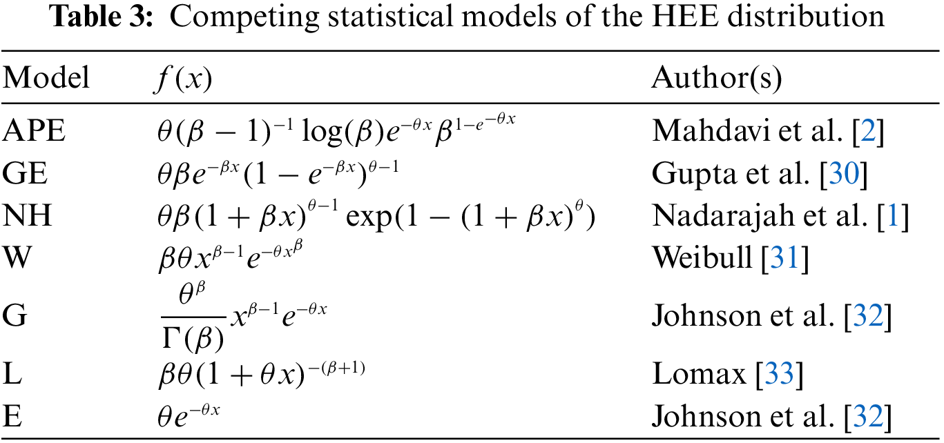
We fit the HEE distribution and compare it to other seven lifetime distributions as its competitors, including the alpha power exponential (APE), generalized-exponential (GE), Nadarajah-Haghighi (NH), Weibull (W), G, Lomax (L), and exponential (E) distributions. For x>0 and β,θ>0, the corresponding PDFs of these distributions are presented in Table 3.

Several model selection criteria, including negative log–likelihood (NL), Akaike’s (A), Bayesian (B), consistent Akaike’s (CA), and Hannan–Quinn (HQ) information criteria, are utilized to show the HEE distribution’s utility in comparison to its rival models. Three alternative goodness–of–fit statistics, namely, Anderson–Darling (AD), Cramér–von Mises (CvM), and Kolmogorov–Smirnov (KS) (with its p-value) statistics are also used to assess the validity of the HEE model in comparison to other competitor models. Based on these measures, the best distribution corresponds to the lowest value of A, B, CA, HQ, AD, CvM and KS statistics as well as to the highest p-value via ℛ software and ‘AdequacyModel’ package proposed by Marinho et al. [34], all unknown parameters are estimated using the maximum likelihood method and their standard–errors (St.Errs) are also computed and reported in Table 4. However, the estimated values of the given goodness–of–fit measures under the turbochargers data set are presented in Table 5. It is evident that the HEE distribution is the good distribution compared to the other distributions under the turbochargers data. We further draw quantile–quantile plots of the HEE distribution and the competitive models based on the same given data, see Fig. 8. Moreover, the histogram and the fitted densities as well as the plot of fitted/empirical reliability functions of all considered distributions are displayed in Figs. 9a and 9b, respectively. Graphical presentations in Figs. 8 and 9 support the results in Table 5 which indicate that the HEE distribution is the best model to fit the turbochargers data compared to all given distributions listed in Table 3.

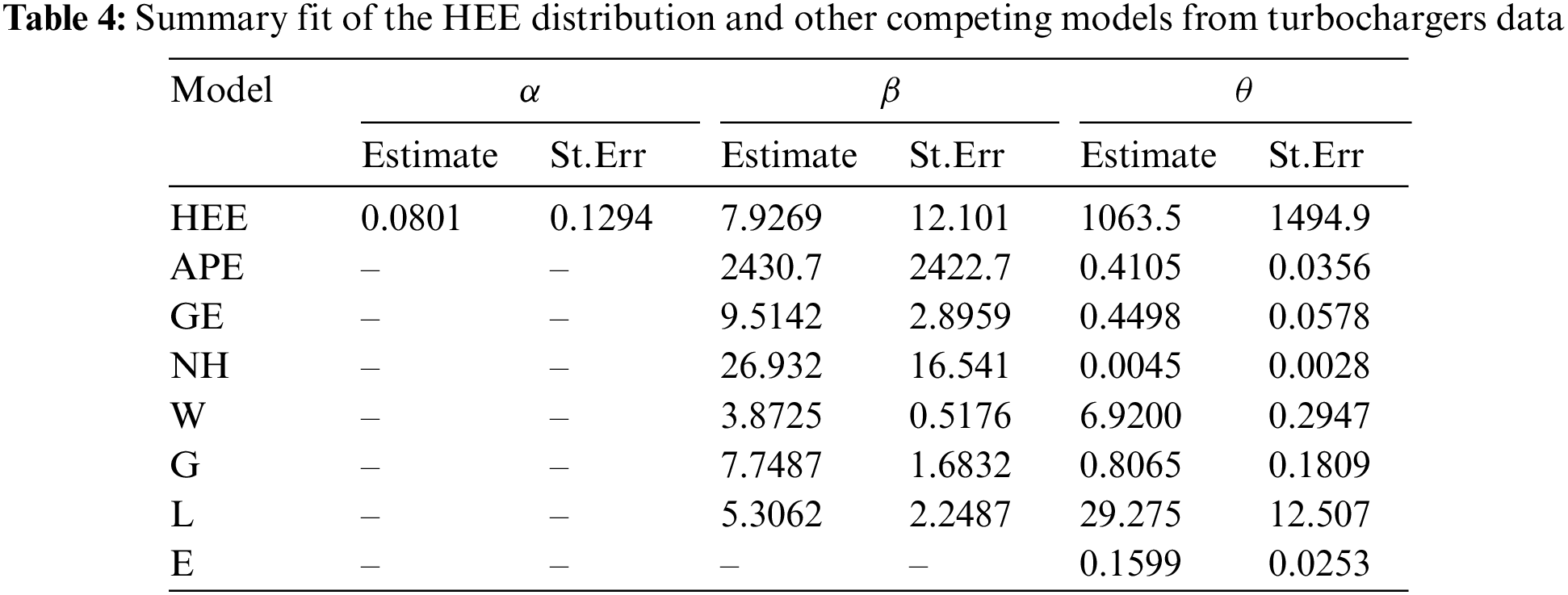
Figure 8: The quantile-quantile plots of the HEE distribution and other competing models using turbochargers data

Figure 9: Estimated densities and reliability functions of the HEE distribution and other competing models using turbochargers data

From the complete turbochargers data, three different progressively Type-II censored samples with m=20 are generated, where R=(2,0,0,0,2) is denoted by R=(2,0∗3,2) and reported in Table 6. Using Table 6, the maximum likelihood and Bayes estimates with their St.Errs of α, β, θ, R(t) and h(t) at given time t=5 are calculated and provided in Table 7. Also, 95% two-sided ACI and HPD credible interval estimates with their interval lengths are obtained and presented in Table 8.

Since no prior information is available for HEE parameters α, β and θ from turbochargers data, non-informative priors, i.e., ai=bi=0, i=1,2,3, are used to carry out the Bayesian analysis from both SE and GE (for δ(=−3,−0.03,+3)) loss functions. To run calculations, we have taken 1×10−4 for all given hyper-parameters. Using the MCMC algorithm described in Section 3, the first 10,000 iterations have been discarded from 50,000 MCMC samples in order to eliminate effects from the initial values. The initial guesses of α, β and θ were taken to be their classical estimates. It is observed, from Tables 7 and 8, that the Bayes estimates of α, β, θ, R(t) and h(t) perform better than the frequentist estimates in terms of their St.Errs as well as the corresponding lengths of the HPD interval estimates are narrow down compared to the ACIs. In addition, some vital properties for the MCMC outputs of all unknown parameters after burn-in, namely: mean, mode, quartiles (Qi for i=1,2,3), standard deviation (St.D) and skewness (Skew.) are calculated and presented in Table 9.

In MCMC iterations, the convergence of simulated chains of each unknown parameter must be checked. Therefore, based on the data set of S1 as an example, trace plots based on 40,000 chain values of α, β, θ, R(t) and h(t) are plotted and displayed in Fig. 10. Furthermore, the associated histograms using the Gaussian kernel for 40,000 MCMC iterations of α, β, θ, R(t) or h(t) are also shown in Fig. 10. For specification, in each trace plot, the sample mean and two bounds of 95% HPD interval are expressed by soled and dashed horizontal lines, respectively, as well as in each histogram plot, the sample mean is plotted by vertical dash–dotted line. Fig. 10 shows that the proposed MCMC algorithm converges well and the size of burn–in sample is enough to eliminate the effect of the initial guesses. It also demonstrates that the generated posteriors of α, β, θ, R(t) and h(t) behave almost symmetrically. In the supplementary file (see Figs. S1–S2), the MCMC plots obtained from samples S2 and S3 of α, β, θ, R(t) and h(t) are presented.

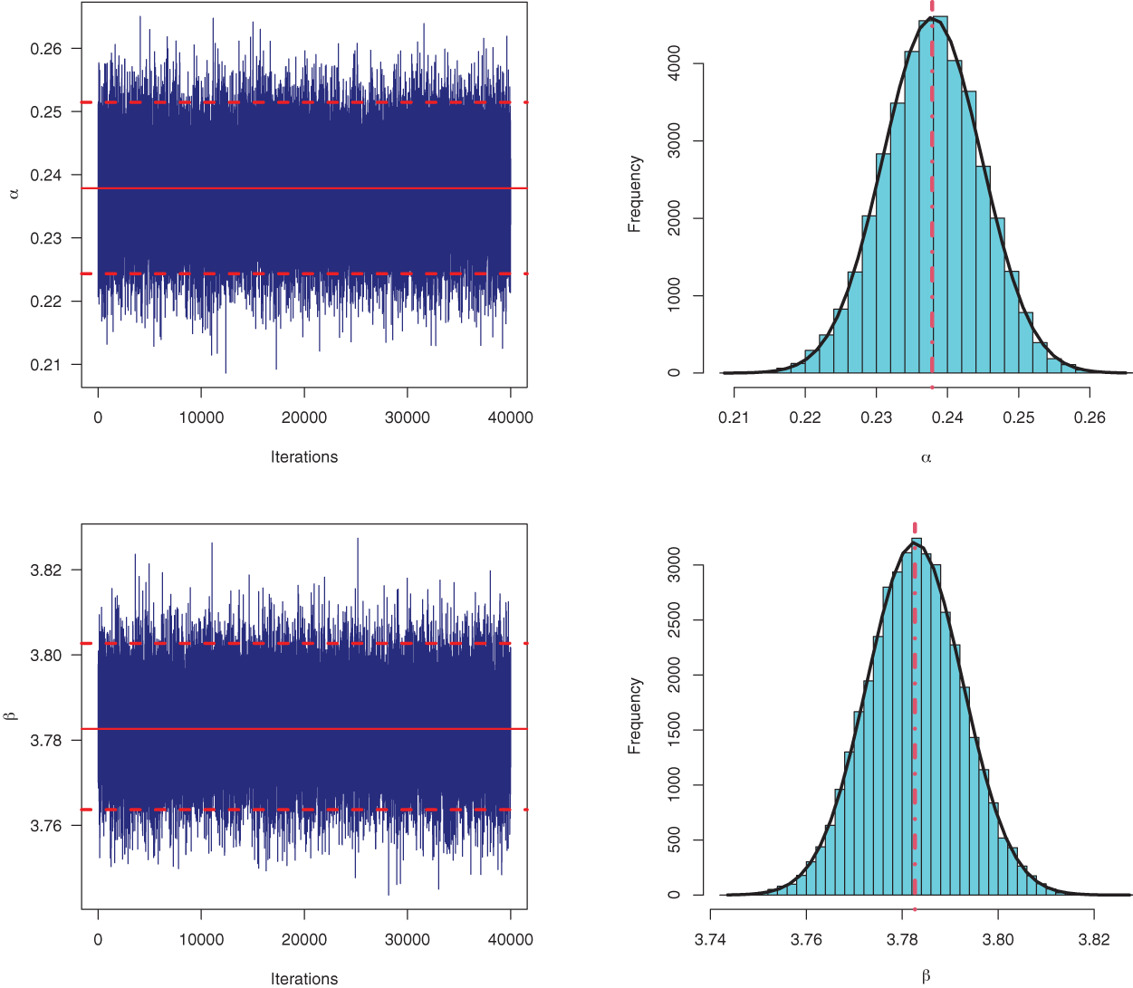
Figure 10: Trace plots (left) and Histogram plots (right) for simulated MCMC samples of α, β, θ, R(t) and h(t) from turbochargers data

On the basis of the data from the turbochargers, the problem of selecting the optimal censoring scheme out of all available censoring methods is also examined. The recommended optimum criteria in Table 1 are determined from the generated samples reported in Table 6 and listed in Table 10. It is clear that the progressive censoring plan (0∗9,10,10,0∗9) is the optimum censoring than others based on the given criterion I, II and III while (10,10,0∗18) is the optimum censoring than others based on the criterion IV for all specified percentiles.

6.2 Guinea-Pigs Data

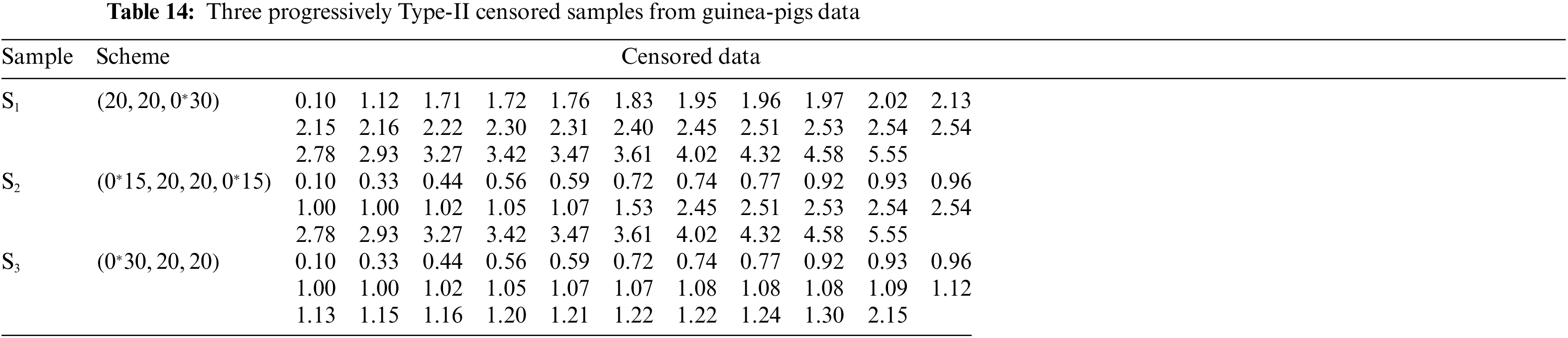
In this application, from veterinary medicine field, we shall provide an analysis for the survival times (in days) of 72 guinea-pigs infected with virulent tubercle bacilli. This data set was originally discussed and reported by Bjerkedal [35] and recently also explained by Chhetri et al. [36]. For computational convenience, each lifetime point in the original guinea-pigs data set is divided by one hundred. In Table 11, the new transformed survival times are reported in ascending order.

Again, to illustrate how the HEE distribution can be used effectively to provide a better fit than the other distributions, the guinea-pigs data set is also analyzed for this purpose. From Table 11, the MLEs (with their St.Errs) of all considered distributions (given in Table 3) are calculated and reported in Table 12. Furthermore, the different goodness-of-fit criteria are also computed and reported in Table 13. It is clear, from Table 13, that the HEE distribution is the best statistical model compared to other fitted models for fitting guinea-pigs data set because it has the lowest values of the different goodness-of-fit measures and the highest p-value. Fig. 11 shows the quantile-quantile plots for the considered distributions. Furthermore, the histogram and the different fitted densities as well as the empirical and fitted reliability functions are displayed in Figs. 12a and 12b, respectively. Figs. 11 and 12 support the same findings reported in Table 13. Now, from the complete guinea-pigs data, different progressively Type-II censored samples with fixed m=32 and various choices of Ri, i=1,…,m are generated and listed in Table 14. The MLEs and the Bayes estimates (with their St.Errs) as well as the 95% ACI/HPD interval estimates (with their lengths) of α, β, θ, R(t) and h(t) (at time t=1) are calculated and reported in Tables 15 and 16, respectively. Using the proposed SE and GE (for δ(=−3,−0.03,+3)) loss functions, because prior knowledge about the HEE parameters from the guinea-pigs data is not available, the Bayes point estimates are obtained based on improper gamma densities when ai=bi=0, i=1,2,3. We also take 0.0001 for all given hyper-parameters. By running the MCMC sampler 50,000 times and omitting the first 10,000 iterations as burn-in, the Bayes point (or interval) calculations are performed. However, Table 15 shows that the point estimates of all unknown parameters obtained by frequentist and Bayesian estimation methods are almost close to each other as expected. A similar finding is also reached in the case of interval estimation.

Figure 11: The quantile-quantile plots of the HEE distribution and other competing models using guinea-pigs data

Figure 12: Estimated densities and reliability functions of the HEE distribution and other competing models using guinea-pigs data

Using the generated sample S1 (as an example) from the guinea-pigs data, both trace and histogram plots for 40,000 MCMC simulated variates of the unknown parameters α, β, θ, R(t) and h(t) are displayed in Fig. 13. It indicates that the MCMC samples generated from all unknown parameters are converged adequately. It is also evident, from the estimated Gaussian kernel, that all the generated posterior samples of the HEE parameters α, β and θ are fairly symmetrical while the generated posteriors of the survival characteristics R(t) and h(t) are negative and positive quite skewed, respectively. Furthermore, some vital statistics of MCMC outputs of α, β, θ, R(t) and h(t) such as: mean, mode, 1st quartile (Q1), 3rd quartile (Q3), St.D and Skew. are computed and presented in Table 17. It shows that the calculated tendency measures support the same application results in Fig. 13. From guinea-pigs data, in the supplementary file (see Figs. S3–S4), the MCMC plots obtained from samples S2 and S3 of α, β, θ, R(t) and h(t) are provided. Moreover, using the specific censoring schemes listed in Table 14, the calculated values of the proposed optimality criteria are provided in Table 18. It shows that the progressive censoring schemes (20,20,0∗30) are the best compared to the other censoring schemes based on criterions IV and II, respectively; and the censoring scheme (0∗30,20,20) is the best compared to the others based on the criterions I and III.

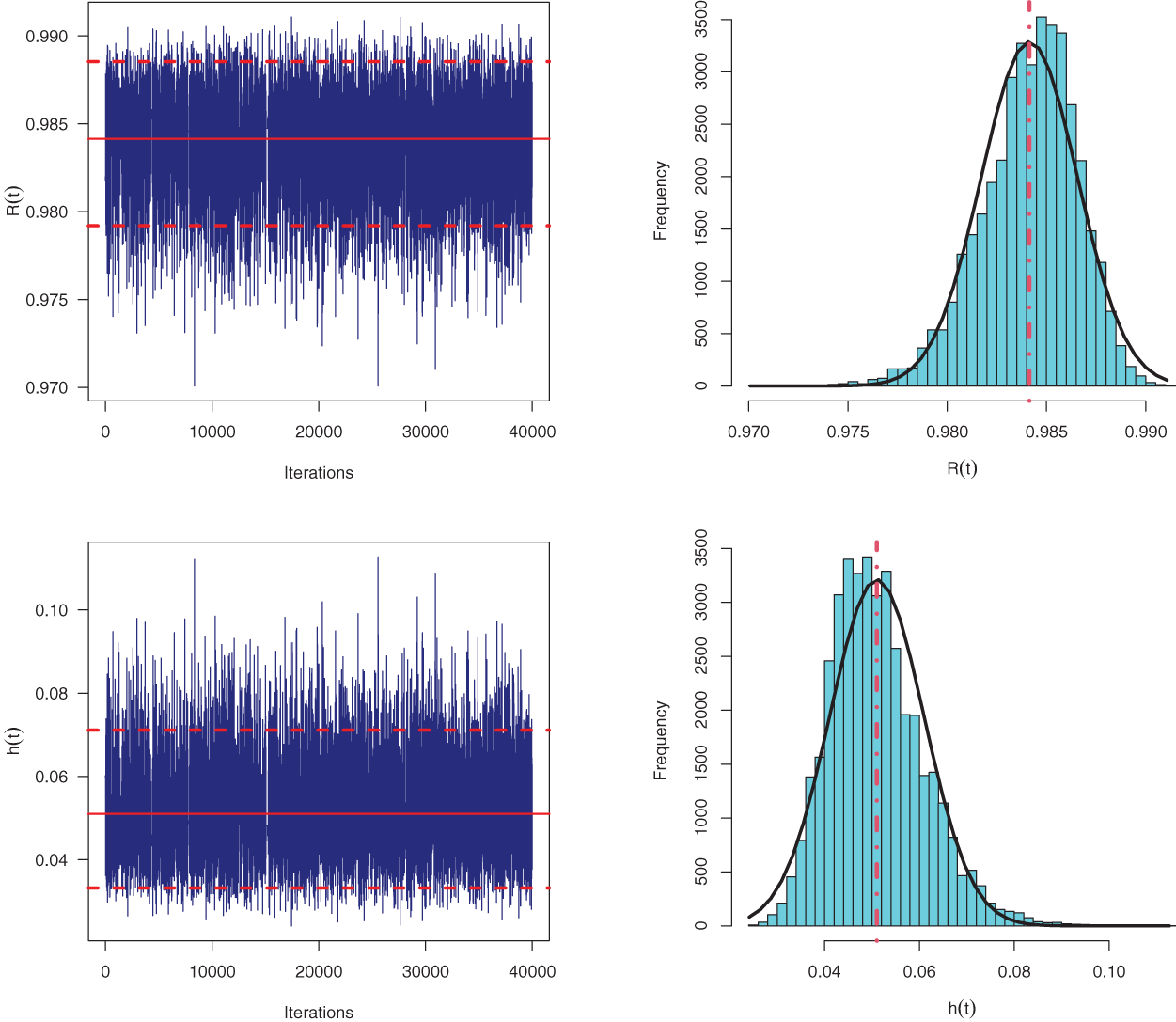
Figure 13: Trace plots (top panel) and Histogram plots (bottom panel) for simulated MCMC samples of α, β, θ, R(t) and h(t) from guinea-pigs data

7  Concluding Remarks

In this work, we have acquired both classical and Bayesian estimations of the Harris extended-exponential distribution in the existence of progressively Type-II censoring samples. The maximum likelihood approach is taken into account in the context of classical estimation in order to get the point and interval estimations of the unknown parameters, reliability, and hazard rate functions. On the other hand, under the premise of independent gamma priors, the Bayesian estimation is created based on both squared and general entropy loss functions. Due to the problematic presentation of the posterior distribution, the Markov Chain Monte Carlo technique is employed to get the Bayes estimates as well as the highest posterior density credible intervals. Monte Carlo simulations are implemented to compare the performance of the diverse point and interval estimators while accounting for various sample sizes and censoring procedures. Some optimality criteria are investigated to discover the best progressive censoring scheme. We examined two data sets for guinea pigs and turbochargers to show how the suggested estimators perform in practical environments. These applications showed also that the Harris extended-exponential distribution provides a better fit than other seven distributions in the literature. To be more specific, the numerical investigations showed that the Bayesian MCMC technique yields more accurate estimates compared to others and is recommended when the progressively Type-II censored Harris extended-exponential data exist. In future work, it may be preferable to reuse the proposed estimation methods to include competing risks or accelerated tests data.

Acknowledgement: The authors would desire to express their gratitude to the editor and the anonymous referees for useful advice and helpful comments. The authors would also like to express their full thanks to Princess Nourah bint Abdulrahman University, Riyadh, Saudi Arabia, for supporting this study.

Funding Statement: This research was funded by Princess Nourah bint Abdulrahman University Researchers Supporting Project Number (PNURSP2023R175), Princess Nourah bint Abdulrahman University, Riyadh, Saudi Arabia.

Conflicts of Interest: The authors declare that they have no conflicts of interest to report regarding the present study.

References

1. Nadarajah, S., Haghighi, F. (2011). An extension of the exponential distribution. Statistics, 45(6), 543–558. [Google Scholar]

2. Mahdavi, A., Kundu, D. (2017). A new method for generating distributions with an application to exponential distribution. Communications in Statistics-Theory and Methods, 46(13), 6543–6557. [Google Scholar]

3. Pinho, L. G. B., Cordeiro, G. M., Nobre, J. S. (2015). The Harris extended exponential distribution. Communications in Statistics-Theory and Methods, 44(16), 3486–3502. [Google Scholar]

4. Marshall, A. W., Olkin, I. (1997). A new method for adding a parameter to a family of distributions with application to the exponential and Weibull families. Biometrika, 84(3), 641–652. [Google Scholar]

5. Sultan, K. S., Alsadat, N. H., Kundu, D. (2014). Bayesian and maximum likelihood estimations of the inverse Weibull parameters under progressive Type-II censoring. Journal of Statistical Computation and Simulation, 84(10), 2248–2265. [Google Scholar]

6. Dey, S., Nassar, M., Maurya, R. K., Tripathi, Y. M. (2018). Estimation and prediction of Marshall–Olkin extended exponential distribution under progressively Type-II censored data. Journal of Statistical Computation and Simulation, 88(12), 2287–2308. [Google Scholar]

7. Kotb, M. S., Raqab, M. Z. (2019). Statistical inference for modified Weibull distribution based on progressively type-II censored data. Mathematics and Computers in Simulation, 162(6), 233–248. [Google Scholar]

8. Bdair, O. M., Awwad, R. R., Abufoudeh, G. K., Naser, M. F. M. (2020). Estimation and prediction for flexible Weibull distribution based on progressive type II censored data. Communications in Mathematics and Statistics, 8(3), 255–277. [Google Scholar]

9. Wu, M., Gui, W. (2021). Estimation and prediction for nadarajah-haghighi distribution under progressive Type-II censoring. Symmetry, 13(6), 999. [Google Scholar]

10. Alotaibi, R., Nassar, M., Rezk, H., Elshahhat, A. (2022). Inferences and engineering applications of alpha power weibull distribution using progressive Type-II censoring. Mathematics, 10(16), 2901. https://doi.org/10.3390/math10162901 [Google Scholar] [CrossRef]

11. Elshahhat, A., Rastogi, M. K. (2022). Bayesian life analysis of generalized chen’s population under progressive censoring. Pakistan Journal of Statistics and Operation Research, 18(3), 675–702. [Google Scholar]

12. Dey, S., Elshahhat, A. (2022). Analysis of Wilson–Hilferty distribution under progressive Type-II censoring. Quality and Reliability Engineering International, 38(7), 3771–3796. [Google Scholar]

13. Balakrishnan, N., Cramer, E. (2014). The art of progressive censoring. Birkhäuser, New York: Springer. [Google Scholar]

14. Henningsen, A., Toomet, O. (2011). maxLik: A package for maximum likelihood estimation in R. Computational Statistics, 26(3), 443–458. [Google Scholar]

15. Panahi, H. (2017). Estimation of the Burr type III distribution with application in unified hybrid censored sample of fracture toughness. Journal of Applied Statistics, 44(14), 2575–2592. [Google Scholar]

16. Panahi, H. (2017). Estimation methods for the generalized inverted exponential distribution under type ii progressively hybrid censoring with application to spreading of micro-drops data. Communications in Mathematics and Statistics, 5(2), 159–174. [Google Scholar]

17. Greene, W. H. (2000). Econometric analysis, 4th edition. New York, NY, USA: Prentice-Hall. [Google Scholar]

18. Meeker, W. Q., Escobar, L. A. (2014). Statistical methods for reliability data. NY, USA: John Wiley & Sons. [Google Scholar]

19. Elshahhat, A., Muse, A. H., Egeh, O. M., Elemary, B. R. (2022). Estimation for parameters of life of the Marshall-Olkin generalized-exponential distribution using progressive Type-II censored data. Complexity, 2022, 36, 8155929. https://doi.org/10.1155/2022/8155929 [Google Scholar] [CrossRef]

20. Dey, S., Elshahhat, A., Nassar, M. (2022). Analysis of progressive type-II censored gamma distribution. Computational Statistics, 38, 481–508. https://doi.org/10.1007/s00180-022-01239-y [Google Scholar] [CrossRef]

21. Nassar, M., Alotaibi, R., Okasha, H., Wang, L. (2022). Bayesian estimation using expected LINEX loss function: A novel approach with applications. Mathematics, 10(3), 436. [Google Scholar]

22. Calabria, R., Pulcini, G. (1994). An engineering approach to Bayes estimation for the Weibull distribution. Microelectronics Reliability, 34(5), 789–802. [Google Scholar]

23. Plummer, M., Best, N., Cowles, K., Vines, K. (2006). CODA: Convergence diagnosis and output analysis for MCMC. R News, 6(1), 7–11. [Google Scholar]

24. Elshahhat, A., Rastogi, M. K. (2021). Estimation of parameters of life for an inverted Nadarajah–Haghighi distribution from Type–II progressively censored samples. Journal of the Indian Society for Probability and Statistics, 22(1), 113–154. [Google Scholar]

25. Ng, H. K. T., Chan, C. S., Balakrishnan, N. (2004). Optimal progressive censoring plans for the Weibull distribution. Technometrics, 46(4), 470–481. [Google Scholar]

26. Kundu, D. (2008). Bayesian inference and life testing plan for the Weibull distribution in presence of progressive censoring. Technometrics, 50(2), 144–154. [Google Scholar]

27. Pradhan, B., Kundu, D. (2009). On progressively censored generalized exponential distribution. Test, 18, 497–515. [Google Scholar]

28. Guerra, R. R., Peña-Ramírez, F. A., Cordeiro, G. M. (2021). The Weibull Burr XII distribution in lifetime and income analysis. Anais da Academia Brasileira de Ciências, 93(3), 1–28. [Google Scholar]

29. Xu, K., Xie, M., Tang, L. C., Ho, S. L. (2003). Application of neural networks in forecasting engine systems reliability. Applied Soft Computing, 2(4), 255–268. [Google Scholar]

30. Gupta, R. D., Kundu, D. (2001). Generalized exponential distribution: Different method of estimations. Journal of Statistical Computation and Simulation, 69(4), 315–337. [Google Scholar]

31. Weibull, W. (1951). A statistical distribution function of wide applicability. Journal of Applied Mechanics, 18, 293–297. [Google Scholar]

32. Johnson, N., Kotz, S., Balakrishnan, N. (1994). Continuous univariate distributions, 2nd edition. NY, USA: John Wiley and Sons. [Google Scholar]

33. Lomax, K. S. (1954). Business failures: Another example of the analysis of failure data. Journal of the American Statistical Association, 49, 847–852. [Google Scholar]

34. Marinho, P. R. D., Silva, R. B., Bourguignon, M., Cordeiro, G. M., Nadarajah, S. (2019). AdequacyModel: An R package for probability distributions and general purpose optimization. PLoS One, 14, e0221487. [Google Scholar] [PubMed]

35. Bjerkedal, T. (1960). Acquisition of resistance in guinea pies infected with different doses of virulent tubercle bacilli. American Journal of Hygiene, 72(1), 130–148. [Google Scholar] [PubMed]

36. Chhetri, S., Mdziniso, N., Ball, C. (2022). Extended Lindley distribution with applications. Revista Colombiana de Estadística, 45(1), 65–83. [Google Scholar]

Supplementary Materials

Table S1: The average estimates (1st column), RMSEs (2nd column) and MABs (3rd column) of α

Table S2: The average estimates (1st column), RMSEs (2nd column) and MABs (3rd column) of β

Table S3: The average estimates (1st column), RMSEs (2nd column) and MABs (3rd column) of θ

Table S4: The average estimates (1st column), RMSEs (2nd column) and MABs (3rd column) of R(t)

Table S5: The average estimates (1st column), RMSEs (2nd column) and MABs (3rd column) of h(t)

Table S6: The ACLs (1st column) and CPs (2nd column) of 95% ACI/HPD credible intervals of α

Table S7: The ACLs (1st column) and CPs (2nd column) of 95% ACI/HPD credible intervals of β

Table S8: The ACLs (1st column) and CPs (2nd column) of 95% ACI/HPD credible intervals of θ

Table S9: The ACLs (1st column) and CPs (2nd column) of 95% ACI/HPD credible intervals of R(t)

Table S10: The ACLs (1st column) and CPs (2nd column) of 95% ACI/HPD credible intervals of h(t)

Figure S1: Trace plots (left) and Histogram plots (right) for simulated MCMC samples of α, β, θ, R(t) and h(t) using sample S2 from turbochargers data

Figure S2: Trace plots (left) and Histogram plots (right) for simulated MCMC samples of α, β, θ, R(t) and h(t) using sample S3 from turbochargers data

Figure S3: Trace plots (top panel) and Histogram plots (bottom panel) for simulated MCMC samples of α, β, θ, R(t) and h(t) using sample S2 from guinea-pigs data

Figure S4: Trace plots (top panel) and Histogram plots (bottom panel) for simulated MCMC samples of α, β, θ, R(t) and h(t) using sample S3 from guinea-pigs data