Bifurcation Analysis of a Nonlinear Vibro-Impact System with an Uncertain Parameter via OPA Method

1  Introduction

As it is well known, the phenomena of impacts and dry frictions exist widely in a large number of engineering devices [1–3], which can induce the instability and insecurity of these devices. Thus, studying the dynamical properties has been an epoch-making field for solving the relative problems of these non-smooth devices [4–6]. In the last few years, numerous papers have concentrated on the study of non-smooth systems [4–8], in particular, on vibro-impact systems. This kind of vibro-impact system appears when a moving mass collides with a barrier and its displacement is greater than a critical value.

Various complex impact structures and models were designed and developed in the past decade; the study of these systems was extensively performed. Namely, since the 1960s, the theoretical and experimental analyses of an impact system under periodic excitation have been performed by Masri [8,9]. Based on the local Poincaré mapping method, the stabilities of non-smooth systems have been considered by Nordmark [10], Zhang et al. [11], and Jin et al. [12]. Furthermore, the transition phenomena between different bifurcation phenomena of an impact oscillator with viscous damping have been studied by Peterka [13]. Luo et al. [14] have researched the bifurcation characteristic of two-degree-of-freedom vibro-impact systems with weak and strong resonance. The global dynamics have been studied in a vibro-impact system with special friction by Gendelman et al. [15]. The chaotic attractors and the periodic behavior of an inelastic, forced-impact oscillator near subharmonic resonance conditions have been explored by Rounak et al. [16]. Additionally, random factors are unavoidable in the operation of dynamical systems [17,18]. By means of the mean Poincaré map, the responses of a vibro-impact system have been analyzed by Feng et al. [19]. By using the non-smooth variable transformation in [20], the energy losses induced by the impact and the probability density functions of the impact systems under stochastic excitation have been considered by Dimentberg et al. [21,22]. An averaging approach to researching the nonlinear dynamics of the vibro-impact system under the effect of random perturbations has been developed by Namachchivaya et al. [23]. Along with researching the multi-valued response of a nonlinear vibro-impact system with the existence of random narrow-band noise [24], Huang et al. have also considered the principal resonances of an elastic impact oscillator under stochastic excitation [25]. The stochastic dynamics of the contact force models with elastic impact phenomena under additive noise have been investigated by Kumar et al. [26]. By using the traditional theoretical analysis, the stochastic dynamical property of a nonlinear vibro-impact system with Coulomb friction under stochastic noise has been researched by Su et al. [27]. Besides investigating the stochastic response of SDOF vibro-impact oscillators under wide-band noise excitations, Qian et al. [28] have also studied the response of vibro-impact systems by the RBF neural network method [29]. Although numerous papers have been published, some stochastic non-smooth systems cannot be investigated by these theoretical methods due to the limited application.

In order to overcome the difficulty of studying dynamical systems with an uncertain parameter, the orthogonal polynomial approximation (OPA) method has been utilized to study the stochastic dynamics of some kinds of smooth dynamical systems [30–32] with uncertain parameters. Although different kinds of orthogonal polynomials can be chosen, the Chebyshev polynomial approximation [30,31] and the Laguerre polynomial approximation [33] are the main methods in the stochastic analysis. By using the method based on the derived approximate formula of the Laguerre polynomials, Wang et al. [33] have investigated the stochastic response of a nonlinear elastic impact system, along with studying the global dynamic behavior of this kind of system with an uncertain parameter [34]. Utilizing the method of Chebyshev polynomial approximation, Feng et al. [35] have studied the bifurcation of a stochastic nonlinear system with a one-sided constraint. Li et al. [36] have considered the bifurcations of the van der Pol system with two-side barriers. Recently, Huang et al. [37] and Zhang et al. [38] have extended the Chebyshev polynomial approximation method to study nonlinear harvesters. However, so far there have been only few papers on the non-smooth dynamical systems with the OPA method. Therefore, in this paper, we mainly concentrate on studying the stochastic responses of the vibro-impact system with nonlinear stiffness and damping under an uncertain parameter subjected to periodic impulse excitation and harmonic excitation according to the OPA method.

The remaining part of this paper is organized as follows: the equivalent high-deterministic system is derived by the OPA method in Section 2; in Section 3 the effectiveness of the OPA method is proved. Afterwards, the bifurcation phenomena of the system by means of deterministic numerical methods are studied, summarizing the conclusions listed in Section 4.

2  Orthogonal Polynomial Approximation

As for stochastic vibro-impact system with nonlinear stiffness and damping under periodic impulse excitation and harmonic excitation, the non-smooth property is induced by the existence of a rigid barrier, as shown in Fig. 1, whose non-dimensional differential equation is given as follows:

{x¨−μ(1−x˙2)x˙+ax+cx3=fcos⁡(ωt)+F(t),x<Δ,x˙+=−ηx˙−,x=Δ,(1)

where fcos⁡(ωt) is the harmonic excitation, a is the coefficient of the linear stiffness and c is the coefficient of the nonlinear stiffness. η is the restitution coefficient (0<η≤1). Δ is the rigid constraint constant. μ is an uncertain parameter, denoted as μ=μ¯+σξ in which ξ is a random variable, μ¯ is the mean value, and σ is the intensity of μ.

Figure 1: The schematic of the nonlinear vibro-impact system

Particularly, F(t)=∑j=0∞δ(t−jT)F0(1+a1sin⁡(ω1nt)), T=2π/ω1, a1=1.0, F0=0.1, ω1=1.0. j is an integer. The impulse signal can be obtained by applying the continuous-time signal F0(1+a1sin⁡(ω1nt)) to an electronic switch which closes momentarily every T seconds. When it comes to n=2, Eq. (1) is affected by the constant impulse force (Fig. 2) which influences the system at the time length 2π/ω1. As it can be seen in Fig. 2a, the value of F(t)=0.0 is at most of the points; only at certain times, F(t) is a nonzero constant. However, in case of n=4, the impulse force presents a different property, which is plotted in Fig. 2b.

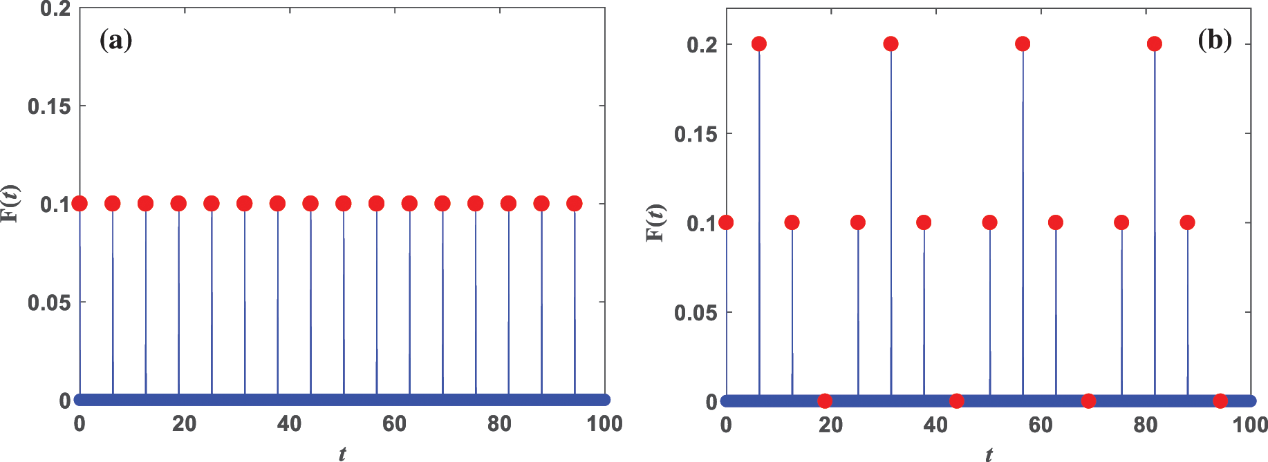
Figure 2: The periodic impulse force F(t) vs. t for F0=0.1. (a) n = 2; (b) n = 4

When the displacement is x<Δ, the system (1) is a stochastic smooth nonlinear system as follows:

x¨−μ(1−x˙2)x˙+ax+cx3=fcos⁡(ωt)+F(t),(2)

When the constraint condition is x<Δ and the constraint plane is H={(x,x˙)|x=Δ}, the jump equation is x˙+=−ηx˙−, x˙− is the velocity before the instant of impacts, and x˙+ is the velocity after the instant of impacts.

According to the OPA method, the responses of the system (1) without the effect of impact can be expanded into the following sequence:

x(t,ξ)=∑i=0Nxi(t)Hi(ξ)(3)

where Hi(ξ) is the ith orthogonal polynomial, herein, the Chebyshev orthogonal polynomials are used [39,40]; N=0,1,2,… is the largest number of the expanded terms: xi(t)=∫−11p(ξ)x(t,ξ)Hi(ξ)dξ and p(ξ)={(2π)1−ξ2,|ξ|≤1,0,|ξ|>1.

The orthogonality of the polynomials is:

∫−112π1−ξ2Hj(ξ)Hi(ξ)dξ={1,i=j,0,i≠j.(4)

Based on the property of the Chebyshev orthogonal polynomials, the recurrent formula among them is:

ξHi(ξ)=12(Hi+1(ξ)+Hi−1(ξ))(5)

As for the case without any constraints, when substituting Eq. (3) into Eq. (2), it has:

(d2dt2−μ¯ddt+a)∑i=0Nxi(t)Hi(ξ)−σξddt(∑i=0Nxi(t)Hi(ξ))+(μ¯+σξ)(ddt(∑i=0Nxi(t)Hi(ξ)))3+c(∑i=0Nxi(t)Hi(ξ))3=fcos⁡(ωt)+F(t).(6)

By Eq. (5), the cubic terms of Eq. (6) can be expanded into a linear combination of the related single polynomials. The coefficient of Hi(ξ) in the linear combination is denoted as Xi(t) and Yi(t),(i=0,1,2,…); thus, the nonlinear terms on the left side of Eq. (6) can be expanded into:

(∑i=0Nxi(t)Hi(ξ))3=∑i=03NXi(t)Hi(ξ),(7)

(ddt(∑i=0Nxi(t)Hi(ξ)))3=∑i=03NYi(t)Hi(ξ).(8)

The expressions of Xi(t) and Yi(t)(i=0,1,2,…) can be derived using software or manual calculation.

Substituting Eqs. (5), (7) and (8) into Eq. (6), the following can be derived:

(d2dt2−μ¯ddt+a)∑i=0Nxi(t)Hi(ξ)−σ2ddt(∑i=0N(xi−1(t)+xi+1(t))Hi(ξ))+μ¯(∑i=03NYi(t)Hi(ξ))+σ2(∑i=03N(Yi−1(t)+Yi+1(t))Hi(ξ))+c(∑i=03NXi(t)Hi(ξ))=fcos⁡(ωt)+F(t).(9)

In order to simplify Eq. (9), both sides of Eq. (9) are multiplied by Hi(ξ) and then taken the expectation about ξ by means of the orthogonality of the Chebyshev polynomials, the equivalent deterministic equation without any constraints can be derived:

(d2dt2−μ¯ddt+a)x0(t)−σ2ddt(x−1(t)+x1(t))+μ¯Y0(t)+σ2(Y−1(t)+Y1(t))+cX0(t)=fcos⁡(ωt)+F(t),(10)

(d2dt2−μ¯ddt+a)x1(t)−σ2ddt(x0(t)+x2(t))+μ¯Y1(t)+σ2(Y0(t)+Y2(t))+cX1(t)=0,(11)

(d2dt2−μ¯ddt+a)x2(t)−σ2ddt(x1(t)+x3(t))+μ¯Y2(t)+σ2(Y1(t)+Y3(t))+cX2(t)=0,(12)

……(d2dt2−μ¯ddt+a)xN(t)−σ2ddt(xN−1(t)+xN+1(t))+μ¯YN(t)+σ2(YN−1(t)+YN+1(t))+cXN(t)=0,(13)

where x−1, xN+1, Y−1 and YN+1 are supposed to be zero due to the approximation in Eq. (3). When N→∞ in Eq. (3), ∑i=0Nxi(t)Hi(ξ) is strictly equivalent to x(t,ξ); however, in the real calculation, N is finite and it is also enough to satisfy the basic requirement of the approximation. In the numerical analysis, N=4 will be taken. The expressions of Xi(t),i=0,1,2,3,4,5, which may be used in the discussion, can be found in [37]. Additionally, if the derivative x˙N is denoted as yN, the expressions of Yi(t),i=0,1,2,3,4,5 are given as follows:

Y0(t)=3y0y12+3y0y22+3y0y32+3y0y42+3y2y32+y03+y23+y43  +3y2y42+3y2y12+3y4y22+3y4y32+6y1y2y3+6y1y3y4(14)

Y1(t)=6y3y22+6y1y32+3y3y12+6y1y22+6y3y42+2y13+2y33+3y1y02  +6y1y42+12y2y3y4+6y0y1y2+6y0y2y3+6y0y3y4+6y1y2y4(15)

Y2(t)=3y23+3y43+3y0y12+3y4y12+3y2y02+3y0y22+6y0y1y3+9y4y32+3y0y32+3y0y42  +6y4y22+6y0y2y4+6y2y12+12y1y2y3+12y1y3y4+9y2y42+9y2y32(16)

Y3(t)=y13+4y33+3y3y02+6y1y32+6y1y22+6y1y42+9y3y22+12y1y2y4  +6y0y1y4+6y0y1y2+6y0y3y4+6y0y2y3+18y2y3y4(17)

Y4(t)=2y23+5y43+3y2y12+3y0y22+3y0y32+3y0y42+12y1y2y3+12y1y3y4  +3y4y02+6y0y2y4+6y0y1y3+6y4y12+9y2y32+9y4y22+9y2y42+12y4y32(18)

Y5(t)=3y33+3y1y22+3y3y12+6y1y42+6y1y32+12y3y42+12y1y2y4  +6y3y22+6y0y2y3+6y0y3y4+6y0y1y4+18y2y3y4(19)

Since ξ is a random variable, when a group of sample {ξi} is taken between −1 and 1, each sample ξi corresponds to a deterministic sample system (2); thus, it is necessary to take the mean value to the sample system. The ensemble mean response (EMR) of the stochastic vibro-impact system can be derived by Eq. (3):

E[x(t,ξ)]=∑i=0Nxi(t)E[Hi(ξ)]=x0.(20)

By means of Eq. (20), the following relations can be defined:

the mean constraint condition

E[x(t,ξ)]=x0=Δ,(21)

the mean constraint plane

H0={(x,x˙)|E[x(t,ξ)]=x0=Δ},(22)

and the mean jump condition

E[x˙+(t,ξ)]=−ηE[x˙−(t,ξ)]⇔x˙0+=−ηx˙0−.(23)

Substituting Eqs. (9)–(13) and (21)–(23) into the system (1), the stochastic nonlinear vibro-impact system can be simplified as follows: in case of x<Δ,

(d2dt2−μ¯ddt+a)x0(t)−σ2ddtx1(t)+μ¯Y0(t)+σ2Y1(t)+cX0(t)=fcos⁡(ωt)+F(t),(24)

(d2dt2−μ¯ddt+a)x1(t)−σ2ddt(x0(t)+x2(t))+μ¯Y1(t)+σ2(Y0(t)+Y2(t))+cX1(t)=0,(25)

(d2dt2−μ¯ddt+a)x2(t)−σ2ddt(x1(t)+x3(t))+μ¯Y2(t)+σ2(Y1(t)+Y3(t))+cX2(t)=0,(26)

…(d2dt2−μ¯ddt+a)xN(t)−σ2ddtxN−1(t)+μ¯YN(t)+σ2YN−1(t)+cXN(t)=0.(27)

and in case of x=Δ, the relationship is given as follows:

x˙0+=−ηx˙0−.(28)

Eqs. (24)–(28) are the equivalent high-dimensional deterministic systems derived by the mean jump equation, the mean constraint condition, and the Chebyshev polynomial approximation. Consequently, the numerical results of the system with an uncertain parameter can be obtained by effective numerical methods.

3  Bifurcation Analysis

3.1 Deterministic Response

Naturally, in the deterministic case the parameters σ=0.0 or ξ=0.0 are satisfied; hence, the original system can be reduced to a deterministic one-side constraint system as follows:

{x¨−μ¯(1−x˙2)x˙+ax+cx3=fcos⁡(ωt)+F(t),x<Δ,x˙+=−ηx˙−,x=Δ.(29)

Due to the deterministic property of Eq. (29), the response can be named the deterministic response (DMR). Therefore, for the equivalent system in Eqs. (24)–(28), by setting the parameter σ=0.0, the deterministic response of the high-dimensional system can be derived and denoted by EMR0. Correspondingly, the stochastic response of the equivalent system is denoted as EMR. Thus, the validity of the polynomial approximation for this kind of vibro-impact system with nonlinear stiffness and damping can be verified by comparing EMR0 with DMR. The differences between EMR and DMR can show the effect of the uncertain parameter on the responses.

In order to calculate the response, the initial condition of Eq. (29) is chosen as x(0)=−1.0, x˙(0)=0.0. In addition, the initial condition of Eqs. (24)–(28) could be obtained as x(0)=[−1.0,0.0,0.0,0.0], x˙(0)=[0.0,0.0,0.0,0.0]. The parameters of the system are given as follows: f=2.0, ω=2.8, a=1.0, μ¯=0.8, η=0.8, Δ=0.0, n=2.

Here, two different Poincaré sections (the phase plane and the constraint plane) are taken, while the value of c varies between 0.01 and 0.1. The bifurcation diagrams are plotted in Fig. 3. It depicts that the properties are the same in Figs. 3a and 3b, having been derived based on different Poincaré sections. In order to verify the response results in Fig. 3, the phase portraits, the time histories, and the Poincaré sections are exhibited in Fig. 4. As Fig. 4 displays, when c increases from 0.035 to 0.05, the 4/4 periodic response of the system converts into the 2/2 response with the asterisk presenting the points of the Poincaré sections. It is also verified the bifurcation properties shown in Fig. 3, which are depicted by the points (A1A2A3A4, C1C2C3C4, B1B2, D1D2). In the symbol z=n/p, p is the number of impacts and n is the number of the periods of the excitation force with the period T=2π/ω. Furthermore, the DMR and EMR0 also present very well the consistent base on the phase portraits in Fig. 4, showing the availability of the approximation method in Section 2.

Figure 3: Bifurcation diagrams of DMR and EMR0 vs. c, (a) the phase plane as Poincaré section, (b) the constraint plane as Poincaré section

Figure 4: (a) The phase portraits and Poincaré sections for c=0.05, (b) the time histories for c=0.05, the periodic 2/2 motion, (c) the phase portraits and Poincaré sections for c=0.035, (d) the time histories for c=0.035, the periodic 4/4 motion

3.2 Effects of an Uncertain Parameter on Period-Doubling Bifurcation

In order to consider the effects of an uncertain parameter on period-doubling bifurcation, the following system parameters are chosen: a=0.5, c=0.05, F0=0.1, f=1.5, u=0.8, η=0.8, Δ=0.0, and n=2. When the excitation frequency ω changes between 3.98 and 4.2, two examples of numerical results are obtained as displayed in Fig. 5 for σ=0.0. Taking the value of ω=3.98, the response characteristics of DMR and EMR0 are obtained as shown in Fig. 5a. Moreover, with increasing ω, DMR and EMR0 from the periodic 6/2 motion turn to the approximate 3/1 motion. As for Poincaré section, the mark “▪” presents the corresponding Poincaré section, and the periodic properties also can be observed clearly from Poincaré section.

Figure 5: The phase portraits (a) ω=3.98, the periodic 6/2 motion, (b) ω=4.2, the periodic 3/1 motion

As for ω=3.98, when the random intensity σ increases to 0.01, the phase portrait can be seen as plotted in Fig. 6a. Even though, the trajectory of the system has certain diffusion, it does not change the property of the motion, the period is still 6T. With the further increase of σ, EMR in Fig. 6b greatly differs from DMR in Fig. 5a; actually, it is no longer the periodic motion under the strict sense. For the case of ω=4.2, it also appears to be the same phenomenon, which is plotted in Figs. 6c and 6d for σ=0.02 and σ=0.03, respectively. Evidently, the strong diffusion phenomenon results in the change of the topological property of the response in Fig. 6d.

Figure 6: EMR for different values of σ as (a) ω=3.98, σ=0.01, (b) ω=3.98, σ=0.014, (c) ω=4.2, σ=0.02, (d) ω=4.2, σ=0.03

As a conclusion, under the effect of the uncertain parameter with the decreasing frequency ω from 4.2 to 3.98, the nonlinear vibro-impact system, just like the deterministic system, experiences a period-doubling bifurcation from 3T to 6T. However, if random intensity continues to increase, the dynamical behavior of the system will experience the essential change. The random factors result in the essential change of the dynamical behavior, the reason of this change is that the trajectories of the system are much closer to the constraint plane; thus, under the random disturbance the trajectories induce diffusion and just impact the constraint plane.

3.3 Existence of Grazing Bifurcation

In this section, to investigate the grazing bifurcation which is typical for the system with impact phenomenon, the same parameters are taken as in Section 3.1, except for a=3.5, f=3.5.

When the frequency is ω=4.00495, as presented in Fig. 7, one trajectory of the system is tangent to the constraint plane with zero speed, and grazing bifurcation occurs which generally exists only in non-smooth systems. However, in this case with increasing the random intensity σ, the phase portraits undergoes a few changes; as shown in Fig. 7. Actually, at some critical points the non-smooth dynamical response becomes insensitive around the grazing point. Even with relatively large disturbance, the system can also keep the original motion state quiet well (Fig. 7b).

Figure 7: EMR for different values of σ as ω=4.00495, (a) σ=0.1; (b) σ=0.2

At the same time, in case of ω=3.98, the phenomenon of grazing bifurcation also occurs, as shown in Fig. 8, but it differs from the case of ω=4.00495 in Fig. 7. When σ=0.1, the trajectories of the system experience certain diffusion in Fig. 8a, and then there is a serious diffusion for bigger σ (as shown in Fig. 8b for σ=0.18). This shows that at this grazing bifurcation point, the effect of the uncertain parameter on the response occurs in the same phenomena with period-doubling bifurcation.

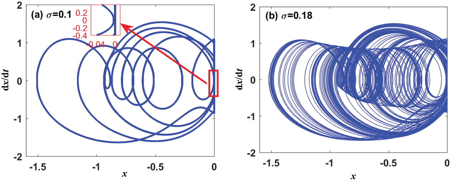
Figure 8: EMR for different values of σ as ω=3.98, (a) σ=0.1, (b) σ=0.18

In order to present the effect of an uncertain parameter on bifurcation, for different values of intensity σ, the bifurcation diagrams of EMR with the variation of ω are plotted in Figs. 9a–9d, respectively. The reasons for the diffusion of the system trajectories are that, on the one hand, the trajectories of the system are much closer to the constraint plane; thus, under the random disturbance the trajectories experience diffusion and then impact the constraint plane. On the other hand, with increasing random intensity σ, the grazing bifurcation appears in advance, which can be seen in Fig. 9.

Figure 9: The bifurcation diagrams of EMR vs. ω for different values of σ, (a) σ=0.0; (b) σ=0.1; (c) σ=0.16; (d) σ=0.18

3.4 Influence of the Impulse Force

When it comes to the influence of the impulse signal on the bifurcation properties the following ideas are considered: the stronger impulse signals are chosen with F0=10.0; the cases n=2 and n=4 are also considered, respectively; and the fact that the different numbers of n lead to different appearance time and values of impulse. Having compared the bifurcation diagrams plotted in Figs. 2 and 10, the following conclusions can be drawn. As it can be seen, at most of the points, the topological properties have not changed, but the diffusion phenomenon apparently has a stronger impulse force, and under larger values of n the diffusion phenomenon is more obvious.

Figure 10: The bifurcation diagrams of EMR0 vs. c with stronger impulse force, (a) the phase plane as Poincaré section with n=2, (b) the constraint plane as Poincaré section with n=2, (c) the phase plane as Poincaré section with n=4, (d) the constraint plane as Poincaré section with n=4

The phase portraits in Fig. 11 also verify the results. As illustrated, under smaller impulse force, different values of n under the influence of the response are not obvious. With larger value of impulse force and under smaller value of n, the diffusion phenomenon can be noticed; however, larger value of n can induce a serious diffusion phenomenon.

Figure 11: The phase portraits for c=0.0356, (a) F0=0.1, n=2; (b) F0=0.1, n=4; (c) F0=10.0, n=2; (d) F0=10.0, n=4

4  Conclusions

In this paper, the OPA method is applied in the vibro-impact system with an uncertain parameter under periodic impulse excitation and harmonic excitation, and the damping coefficient is considered as an uncertain parameter. In order to study the dynamical response, the ensemble mean response of an equivalent high-dimensional system is introduced and the impact conditions are also transformed by means of the mean value; then, the deterministic high-dimensional equivalent vibro-impact system is derived. Afterward, the constraint plane and the phase plane are chosen as the Poincaré section, respectively, with the response properties being consistent in the bifurcation diagrams. By combining the analysis of the phase portraits, it is evident that the approximation method is effective in this kind of vibro-impact system. Furthermore, it has been proved that besides period-doubling bifurcation, certain grazing bifurcation exists also in the stochastic nonlinear vibro-impact system. Under the influence of the uncertain parameter, the system responds not only with the characteristic of the smooth system which can make trajectories of the systems’ diffusion, but also with a special characteristic of a non-smooth system. At a critical point of bifurcation, the random factors with certain intensity make the dynamical behavior of the system change drastically. Furthermore, grazing bifurcation appears in advance with increasing random intensity. The existence of the stronger impulse force can induce the appearance of a diffusion phenomenon. An appropriate choice of impulse force can control the vibration and improve the response performance. Overall, the bifurcation analysis is helpful for further investigating of stochastic dynamics.

Acknowledgement: The authors are grateful for the support by the National Natural Science Foundation of China, the Bilateral Governmental Personnel Exchange Project between China and Slovenia for the Years 2021–2023, Slovenian Research Agency ARRS in Frame of Bilateral Project, the Fundamental Research Funds for the Central Universities, Joint University Education Project between China and East European.

Funding Statement: This work was supported by the National Natural Science Foundation of China (Grant Nos. 12172266, 12272283), the Bilateral Governmental Personnel Exchange Project between China and Slovenia for the Years 2021–2023 (Grant No. 12), Slovenian Research Agency ARRS in Frame of Bilateral Project (Grant No. P2-0137), the Fundamental Research Funds for the Central Universities (Grant No. QTZX23004), Joint University Education Project between China and East European (Grant No. 2021122).

Author Contributions: The authors confirm contribution to the paper as follows: Conceptualization, Methodology, Validation: Dongmei Huang; analysis and interpretation of results: Dongmei Huang, Dang Hong, Wei Li; Writing-Original Draft: Dongmei Huang, Dang Hong, Wei Li, Guidong Yang and Vesna Rajic. All authors reviewed the results and approved the final version of the manuscript.

Availability of Data and Materials: Data will be made available on request.

Conflicts of Interest: The authors declare that they have no conflicts of interest to report regarding the present study.

References

1. Babitsky, V. I. (1998). Theory of vibro-impact systems and applications. Berlin: Springer Science & Business Media. [Google Scholar]

2. Jin, D., Hu, H. (2005). Vibration and control of collision. Beijing, China: Science Press. [Google Scholar]

3. Nguyen, K. T., La, N. T., Ho, K. T., Ngo, Q. H., Chu, N. H. et al. (2021). The effect of friction on the vibro-impact locomotion system: Modeling and dynamic response. Meccanica, 56, 2121–2137. [Google Scholar]

4. Stefani, G., de Angelis, M., Andreaus, U. (2021). Scenarios in the experimental response of a vibro-impact single-degree-of-freedom system and numerical simulations. Nonlinear Dynamics, 103(4), 3465–3488. [Google Scholar]

5. Hu, D., Xu, X., Guirao, J., Chen, H., Liu, X. (2022). Moment lyapunov exponent and stochastic stability of a vibro-impact system driven by Gaussian white noise. International Journal of Non-Linear Mechanics, 142, 103968. [Google Scholar]

6. Shaw, S. W. (1983). A periodically forced piecewise linear oscillator. Journal of Sound and Vibration, 90(1), 129–155. [Google Scholar]

7. Huang, D., Han, J., Li, W., Deng, H., Zhou, S. (2023). Responses, optimization and prediction of energy harvesters under galloping and base excitations. Communications in Nonlinear Science and Numerical Simulation, 119, 107086. [Google Scholar]

8. Masri, S. F. (1968). Analytical and experimental studies of impact damper. Journal of the Acoustical Society of America, 45, 1111–1117. [Google Scholar]

9. Masri, S. F. (1973). Steady state response of a multidegree system with an impact damper. Journal of Applied Mechanics, 30(3), 127–132. [Google Scholar]

10. Nordmark, A. B. (1991). Non-periodic motion caused by grazing incidence in an impact oscillator. Journal of Sound and Vibration, 145(2), 279–297. [Google Scholar]

11. Zhang, S., Lu, Q. (2000). A non-smooth analysis to the rub-impacting rotor system. Acta Physica Sinica, 32, 59–69. [Google Scholar]

12. Jin, L., Lu, Q. S. (2005). A method for calculating the spectrum of lyapunov exponents of non-smooth dynamical systems. Acta Mechanica Sinica, 37, 40–47. [Google Scholar]

13. Peterka, F. (1996). Bifurcation and transition phenomena in an impact oscillator. Chaos Solitons and Fractals, 7(10), 1635–1647. [Google Scholar]

14. Luo, G., Xie, J. (2004). Periodic motion and bifurcation of vibro-impact systems. Beijing, China: Science Press. [Google Scholar]

15. Gendelman, O., Kravetc, P., Rachinskii, D. (2019). Mixed global dynamics of forced vibro-impact oscillator with Coulomb friction. Chaos, 29(11), 113116. [Google Scholar] [PubMed]

16. Rounak, A., Gupta, S. (2020). Bifurcations in a pre-stressed, harmonically excited, vibro-impact oscillator at subharmonic resonances. International Journal of Bifurcation and Chaos, 30(8), 2050111. [Google Scholar]

17. Huang, D., Han, J., Zhou, S., Han, Q., Yang, G. et al. (2022). Stochastic and deterministic responses of an asymmetric quad-stable energy harvester. Mechanical Systems and Signal Processing, 168, 108672. [Google Scholar]

18. Huang, D., Zhou, S., Li, W., Litak, G. (2021). On the stochastic response regimes of a tristable viscoelastic isolation system under delayed feedback control. Science China Technological Sciences, 64(4), 858–868. [Google Scholar]

19. Feng, Q., He, H. (2003). Modeling of the mean Poincaré map on a class of random impact oscillators. European Journal of Mechanics-A/Solids, 22(2), 267–281. [Google Scholar]

20. Zhuravlev, V. F. (1976). A method for analyzing vibration-impact systems by means of special functions. Mechanics of Solids, 11(2), 23–27. [Google Scholar]

21. Dimentberg, M. F., Iourtchenko, D. V. (2004). Random vibrations with impacts: A review. Nonlinear Dynamics, 36, 229–254. [Google Scholar]

22. Iourtchenko, D. V., Song, L. L. (2006). Numerical investigation of a response probability density function of stochastic vibro-impact systems with inelastic impacts. International Journal of Non-Linear Mechanics, 41(3), 447–455. [Google Scholar]

23. Namachchivaya, N. S., Park, J. H. (2005). Stochastic dynamics of impact oscillators. Journal of Applied Mechanics, 72, 862–870. [Google Scholar]

24. Huang, D., Xu, W., Liu, D., Han, Q. (2016). Multi-valued responses of a nonlinear vibro-impact system excited by random narrow-band noise. Journal of Vibration and Control, 22(12), 2907–2920. [Google Scholar]

25. Huang, D., Xu, W., Xie, W., Han, Q. (2015). Principal resonance response of a stochastic elastic impact oscillator under nonlinear delayed state feedback. Chinese Physics B, 24(4), 040502. [Google Scholar]

26. Kumar, P., Narayanan, S., Gupta, S. (2022). Dynamics of stochastic vibro-impact oscillator with compliant contact force models. International Journal of Non-Linear Mechanics, 144, 104086. [Google Scholar]

27. Su, M., Xu, W., Yang, G. (2018). Response analysis of van der Pol vibro-impact system with Coulomb friction under Gaussian white noise. International Journal of Bifurcation and Chaos, 28(13), 1830043. [Google Scholar]

28. Qian, J., Chen, L. (2021). Random vibration of SDOF vibro-impact oscillators with restitution factor related to velocity under wide-band noise excitations. Mechanical Systems and Signal Processing, 147, 107082. [Google Scholar]

29. Qian, J., Chen, L., Sun, J. (2023). Random vibration analysis of vibro-impact systems: RBF neural network method. International Journal of Non-Linear Mechanics, 148, 104261. [Google Scholar]

30. Ma, S., Xu, W., Li, W., Jin, Y. (2005). Period-doubling bifurcation analysis of stochastic van der Pol system via Chebyshev polynomial approximation. Acta Physica Sinica, 54(80), 3508–3515. [Google Scholar]

31. Sun, X., Xu, W., Ma, S. (2006). Period-doubling bifurcation of a double-well Duffing-van der Pol system with bounded random parameters. Acta Physica Sinica, 55(2), 610–616. [Google Scholar]

32. Ma, S., Xu, W., Li, W. (2006). Analysis of bifurcation and chaos in double-well Duffing system via laguerre polynomial approximation. Acta Physica Sinica, 55(8), 4013–4019. [Google Scholar]

33. Wang, L., Xu, W., Li, G., Li, D. (2009). Response of a stochastic Duffing–Van der Pol elastic impact oscillator. Chaos, Solitons & Fractals, 41(4), 2075–2080. [Google Scholar]

34. Wang, L., Yue, X., Sun, C., Xu, W. (2013). The effect of the random parameter on the basins and attractors of the elastic impact system. Nonlinear Dynamics, 71, 597–602. [Google Scholar]

35. Feng, J., Xu, W., Wang, R. (2006). Period-doubling bifurcation of stochastic Duffing one-sided constraint system. Acta Physica Sinica, 55(11), 5733–5739. [Google Scholar]

36. Li, G., Xu, W., Wang, L., Feng, J. (2008). Investigation of the bifurcation of stochastic van der Pol system. Acta Physica Sinica, 57(4), 2107–2114. [Google Scholar]

37. Huang, D., Zhou, S., Han, Q., Litak, G. (2019). Response analysis of the nonlinear vibration energy harvester with an uncertain parameter. Proceedings of the Institution of Mechanical Engineers Part K: Journal of Multi-Body Dynamics, 234(2), 393–407. [Google Scholar]

38. Zhang, Y., Duan, X., Shi, Y., Yue, X. (2021). Response analysis of the tristable energy harvester with an uncertain parameter. Applied Sciences, 11(21), 9979. [Google Scholar]

39. Kamerich, E. (1999). A guide to Maple. New York: Springer. [Google Scholar]

40. Borwein, P., Erdelyi, T. (2003). Polynomials and polynomial inequality. New York: Springer. [Google Scholar]