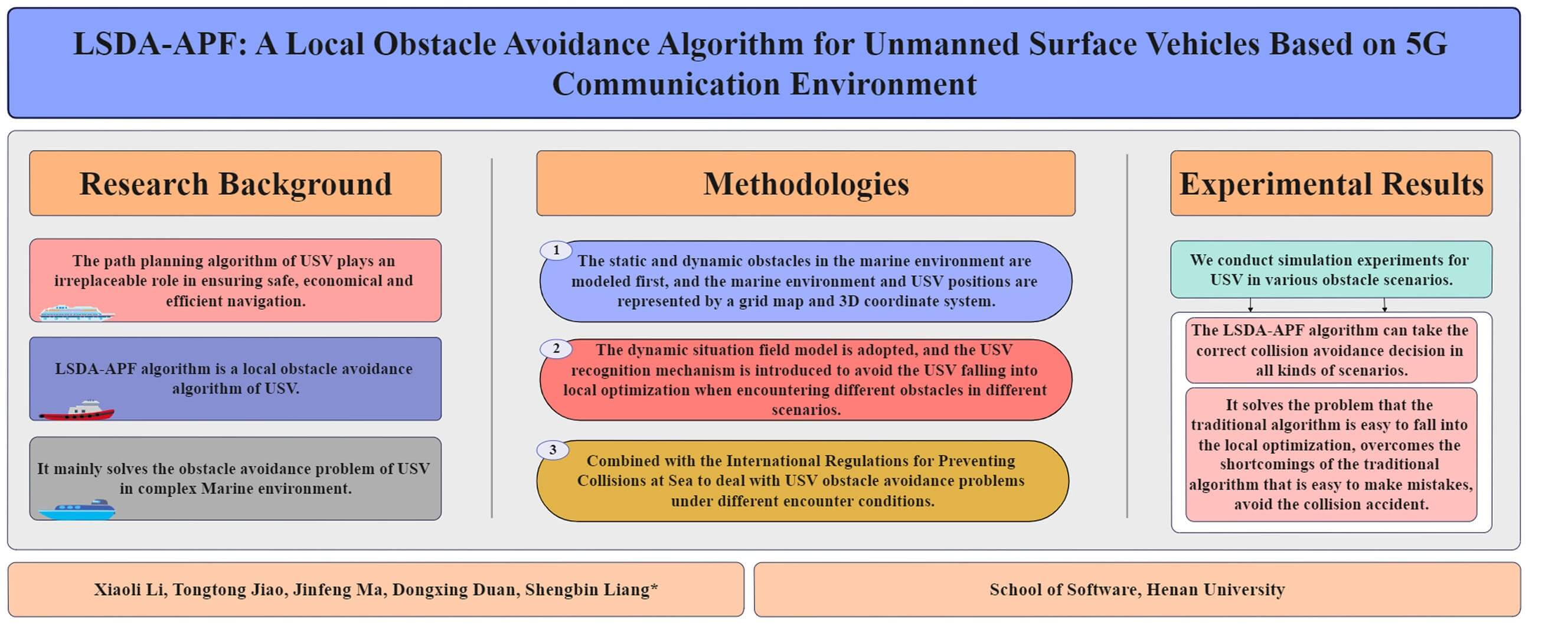
LSDA-APF: A Local Obstacle Avoidance Algorithm for Unmanned Surface Vehicles Based on 5G Communication Environment

1  Introduction

USV is a kind of unmanned control intelligent device equipped with a variety of sensors, radar, and monitoring equipment. A USV system usually consists of three parts: USV, control center, and communication system, as shown in Fig. 1. The USV performs data collection, data transmission, remote control, and other functions through the communication link layer. The USV plays an important role in marine environment mapping [1–3], maritime reconnaissance and surveillance [4], water ecological protection [5], and water search and rescue [6,7]. The USV can improve work efficiency and reduce the casualty probability of operators.

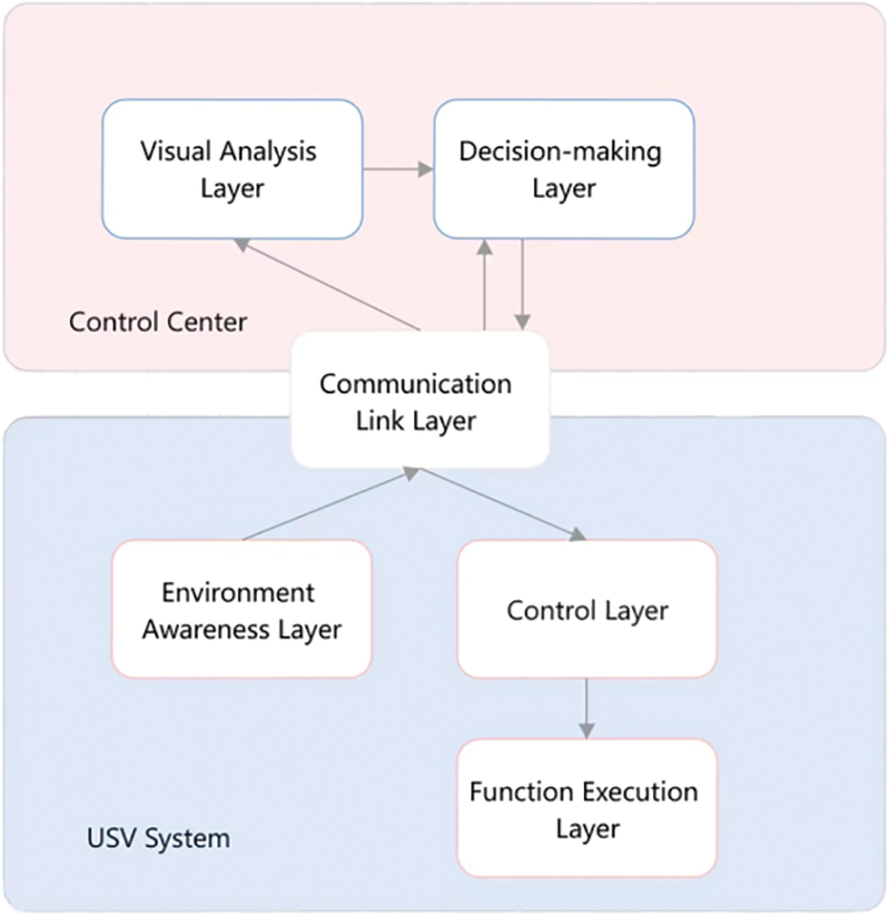
Figure 1: The architecture of USV system

The USV has a high degree of self-control ability. It can perceive the complex environment around it through radar, sonar, and automatic identification system (AIS), dynamically adjust its course and speed, and avoid collisions with static and dynamic obstacles such as vessels during navigation. The path planning algorithm of USV plays an irreplaceable role in ensuring safe, economical and efficient navigation, and is also the core module of the USV system. The path planning algorithms of USV system include global path planning and local obstacle avoidance algorithm. The global path planning is a preliminary path planning in the specified area by using the control center of USV to set the waypoints to be passed before the USV sets off. The global path planning is based on the environment modeling, combined with the obstacle avoidance algorithm to determine the overall path. Since global path planning cannot deal with emergencies during voyaging, such as unknown obstacles and other sailing vessels, the real-time requirement is not high. Global path planning algorithms, such as ant colony algorithm [8] and Dijkstra algorithm [9] can complete the task. The local obstacle avoidance algorithm requires the USV to quickly adjust the preset navigation route to avoid obstacles and return to the global planning route in time according to the feedback of the surrounding environment. Local obstacle avoidance algorithms mainly include APF [10], Dynamic Window Approach (DWA) [11], Velocity Obstacle (VO) [12], Vector Field Histogram (VFH) [13], etc.

The APF algorithm has some advantages of high real-time performance, rapid response and simple calculation. However, if the composite force of a certain position is zero during voyaging, the USV cannot bypass the place, resulting in local optimization. At the same time, when the target is surrounded by obstacles, the path cannot converge, and the USV may not reach the target waypoint. Lyu et al. [14] proposed an improved APF algorithm for path planning in dynamic environment, which solved the collision problem of stationary and moving dangerous objects, COLREGS are also applied, but this method does not consider environmental factors such as wind and waves in the sea. Song et al. [15] proposed a two-level dynamic obstacle avoidance algorithm. VO algorithm was used to establish the velocity vector relationship between USV and obstacles, and APF was used to realize the avoidance method in emergencies. This method defined two strategies, emergency and non-emergency, but the strategy switching and its efficiency in different environments remained to be verified, and environmental conditions such as multiple obstacles were not considered. Fan et al. [16] proposed a moving target detection and avoidance method based on relative velocity based on APF algorithm for a dynamic environment. This method not only considered the spatial position of the moving object, but also considered the velocity and direction of the moving object. It can avoid dynamic obstacles in time, but the real-time performance of this method is not powerful.

The VO method builds a triangle area between the USV and the obstacle based on the velocity space. As long as the velocity vector falls into this triangle area, it is determined that the two will collide. To avoid obstacles, the VO algorithm must find an optimal velocity vector from the non-triangular area and find the optimal path. Ren et al. [17] proposed an autonomous obstacle avoidance algorithm for USV based on improved VO. The algorithm draws on the idea of the velocity obstacle method through the integration of characteristics such as the USV dynamic model in the marine environment, it contains two parts: a multi-vessel encounter collision detection model and a path re-planning algorithm. Simulation results show that the algorithm can enable USVs to safely evade multiple short-range dynamic targets under COLREGS. Aiming at the problem that the VO algorithm does not consider the dynamic obstacles, Kuwata et al. [18] proposed a method to identify the speed and direction of dynamic obstacles based on COLREGS to achieve obstacle avoidance. Wang et al. [19] proposed a special triangular obstacle geometric model to reconstruct the velocity obstacle area. The collision time is predicted by combining the previously collected data with the distance, course and other relevant data of the detected obstacles. Then, determine the start and end time of obstacle avoidance according to the collision risk. Xia et al. [20] proposed a local path planning algorithm based on quantum particle swarm optimization (MQPSO). This method shows that it has good real-time performance, and also considers the energy loss caused by speed change and course adjustment.

DWA is an online obstacle avoidance algorithm, which relies on real-time detection of local information to carry out online planning in a rolling way, and uses heuristic methods to generate optimization sub-goals. With the window rolling to obtain new local information, the algorithm realizes the combination of optimization and feedback in the rolling, and finally realizes local path planning. Zhou et al. [21] proposed a calculation of turning time consumption of DWA based on actual environment. Simulation experiments show that this method can improve the planning ability of USV and enhance the effectiveness of dealing with related path planning problems. Zhang et al. [22] proposed an improved dual-window DWA obstacle avoidance algorithm based on a fuzzy control strategy. That is, on the basis of the conventional speed window, the induction window based on the ship sensor is designed, and the double window model composed of speed window and induction window is further optimized, so that the weight of the cost function can be dynamically adjusted by the fuzzy control strategy for the distribution state and distance of obstacles.

VFH method is a real-time path planning algorithm for the problem that the APF cannot reach the target point when there are obstacles near the target. It models the environment as a grid map and calculates the cost of USV moving forward in each direction. If there are more obstacles in a certain direction, the cost of USV moving forward will be greater. A histogram is established according to the generation value, and the direction with the lowest cost is selected. Ni et al. [23] used wavelet transform technology to de-noise the image collected by USV and used watershed method for segmentation, and proposed an improved VFH method to solve the obstacle avoidance method of USV from high dimension to low dimension in segmented image. Wu et al. [24] used shipborne laser radar to quickly identify dynamic obstacles, and optimize candidate directions by considering USV velocity vector and dynamic obstacles through VFH+ method to avoid obstacles, but this method may still fall into local optimization in solving complex environment. Zhang et al. [25] proposed a method of intelligent vector field histogram (IVFH) to achieve collision avoidance of autonomous underwater vehicle (AUV) in underwater 3D dynamic space. The directed cuboid static obstacle environment model was introduced to improve the efficiency of collision avoidance decision-making. The set of candidate directions consists of relative heading and relative pitch. According to the distribution of local environment obstacles, the driving fitness of each candidate direction is calculated from the perspective of safety and speed, and the collision avoidance of AUV in three-dimensional dynamic environment is realized.

Summarized, different local obstacle avoidance algorithms, when simulating the marine environment including static and dynamic obstacles, USVs are still easy to fall into local optimization when navigating, the real-time performance is not high, and the cost of navigation is high. This paper has done the following two work for the local obstacle avoidance method of USV.

(1)   Real-time perception methods of dynamic and static obstacles in the marine environment are introduced, we use grid map to model the environment, design the objective function, and realize automatic switching between local obstacle avoidance and global path planning.

(2)   The discrimination mechanism is introduced to improve the global potential field function of the artificial potential field algorithm by integrating two evaluation indicators of the lowest working cost and the shortest sailing time. At the same time, the virtual potential field and its calculation method are introduced to realize the local obstacle avoidance algorithm of USV in complex scenes, which effectively reduces the collision risk and the target unreachable problem caused by local optimization under the scenario of multi-vessel encounters. Simulation results show that the improved algorithm proposed in this paper has strong advantages in avoiding local optimization.

The rest of this paper is structured as follows: Section 2 introduces the problem definition and summarizes the two sub-problems to be solved for USV local obstacle avoidance. Section 3 introduces the USV local autonomous obstacle avoidance algorithm based on the improved APF algorithm. Section 4 gives simulation experiment and result analysis. Section 5 summarizes this work.

2  Problem Definition

2.1 Modelling of Dynamic Environment

The 5G communication device of the USV designed in this paper can report the position of the USV to the control center at a time interval of 1 s, and the AIS system integrated by the USV can sense the direction and speed of other vessels in the surrounding environment. We introduce a three-dimensional coordinate system to construct the real-time position of USV. x and y represent the latitude and longitude of USV, respectively, and the position of USV at time t can be represented by (xt,yt), as shown in Fig. 2.

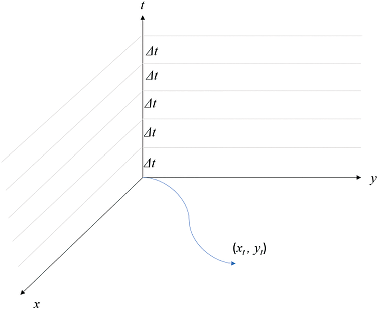
Figure 2: USV location representation based on 3D coordinates

Then, the real-time coordinate position of the USV can be expressed as follows:

xt=xt−1+vt−1⋅Δt⋅cos⁡φ

yt=yt−1+vt−1 ⋅ Δt⋅sin⁡φ(1)

where xt, yt are the coordinate position of USV at time t, and Δt is the time interval, which is 1 s by default in this paper, φ is the direction of navigation.

For the distance between USV and obstacles, we use Eq. (2) calculate the Euclidean distance.

dist=(xusv−xobs)2+(yusv−yobs)2(2)

Fig. 3 shows the steering system of the USV system. In order to ensure the safety during the navigation, the relative navigation angle φ between two USVs is used to distinguish the states that the USV will encounter. The calculation method of φ is shown in Eq. (3),

φ=arctan⁡(xusv(ti)−xobs(ti)yusv(ti)−yobs(ti))+ φusv(3)

where (xusv, yusv) is the position of the USV at time ti, (xobs, yobs) is the coordinate position of the obstacle, φusv is the heading angle of the current USV. The minimum safe distance for obstacle avoidance should be set during the navigation of USV, that is, the threshold m. When the distance between another USV performing a task and the obstacle vessel is less than safe distance m, the heading of USV should be adjusted in the following three cases, as shown in Fig. 4.

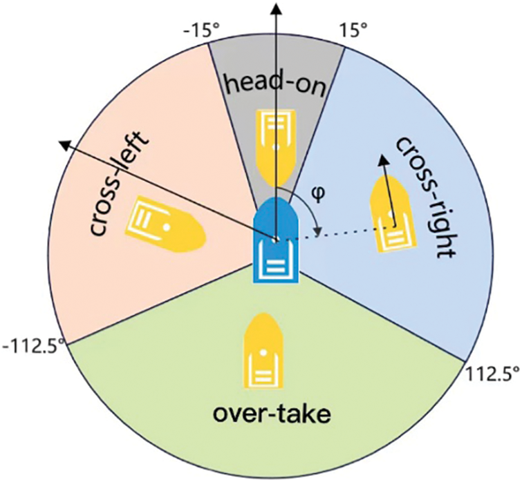
Figure 3: USV steering system

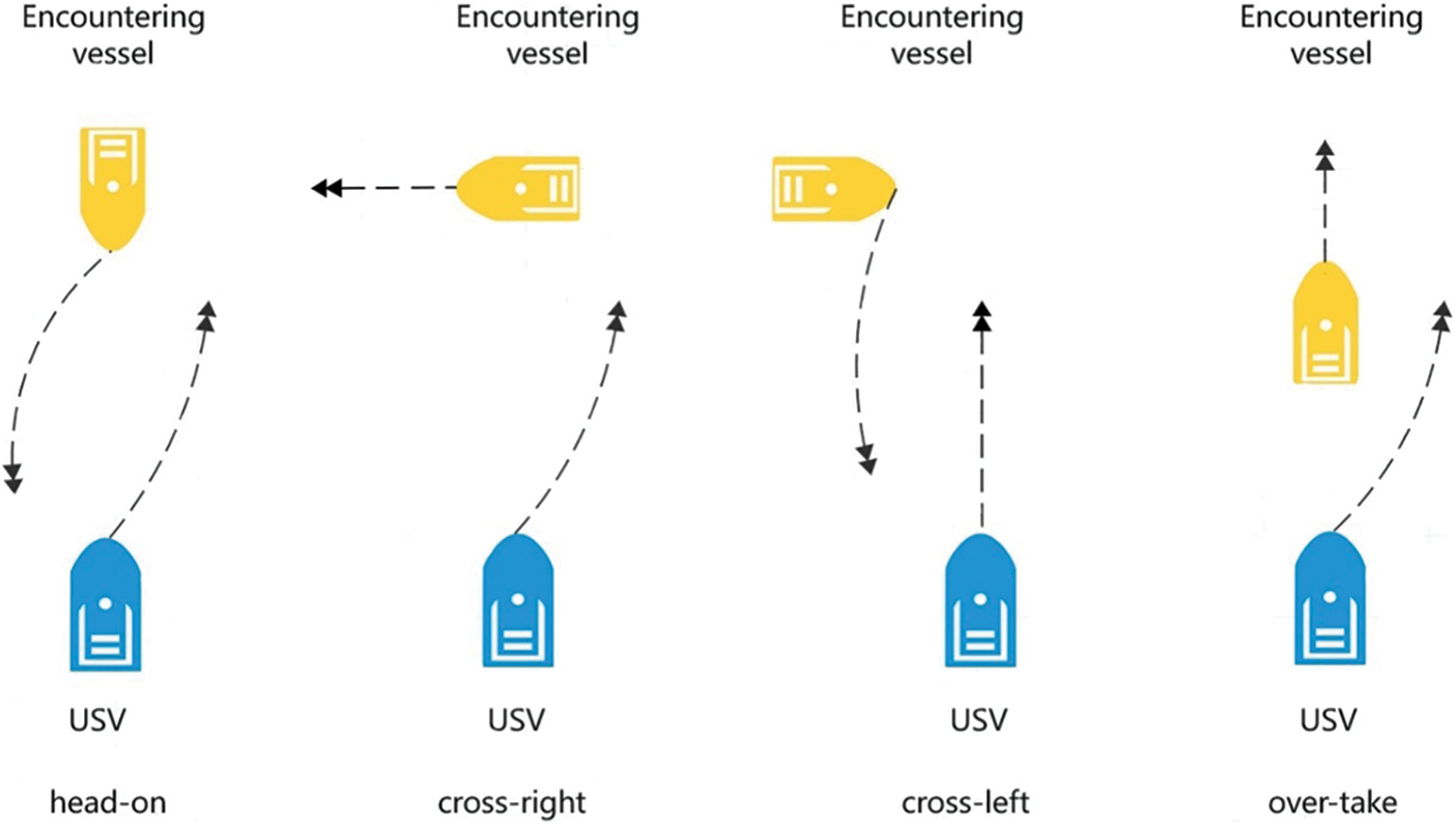
Figure 4: Obstacle avoidance diagram based on COLREGS

(1)   Head-on: When the USV meets the obstacle vessel in the opposite or nearly opposite course and the distance is less than the minimum safety distance, each vessel shall turn to the right and pass the other vessel on the port side; The USV should adjust the heading angle φ to the right.

(2)   Over-take: When the USV over-takes the obstacle vessel in front, the USV can adjust the heading angle φ to the right when it is determined that it is safe to turn.

(3)   Crossing: When two vessels cross each other in the minimum safe distance range, if the obstacle vessel is on the starboard side of the USV, the USV will adjust the heading angle φ to the right or stop; if the USV is on the starboard side of the obstacle vessel, the USV may maintain the same course and the obstacle vessel should alter its course or stop.

The USV obstacle avoidance system sets the safe distance threshold according to the scenario between the two waypoints and the speed of the two encountered vessels. When there are many static obstacles between two waypoints or the USV speed is high, the minimum safe distance is appropriately increased to improve the safety of USV navigation. In these obstacle avoidance scenarios shown in Fig. 4, the basic strategy is to appropriately reduce the safe distance threshold when there are few static obstacles or the USV speed is slow, so as to improve the navigation economy and distance cost of USV. At the same time, in order to avoid collision and improve the efficiency of USV, the safe distance threshold of the algorithm proposed in this paper must be greater than or equal to the influence radius of static obstacles when setting the minimum safe distance of USV’s obstacle avoidance system. When the USV enters the obstacle avoidance state, it adjusts the heading angle according to the environment, and then drives along the current heading at a prosper speed. When the distance between the two USVs is greater than the minimum safe distance, the USV collision avoidance state ends and jumps out of the obstacle avoidance state.

2.2 Modelling of Static Environment

Static environment modeling is a very important initial work in obstacle avoidance algorithms, its goal is to map the real space into an abstract space that can be represented and computed by algorithms. Traditional environment modeling methods include topological graph method [26], Voronoi diagram method [27], cell tree method [28], grid method [29] and other graph theory representation methods. In this paper, the static environment is described by grid map, which divides the navigation area into a series of grid cells with binary information, and the octree is used to represent the environment of the grid. In the grid map, the grid with obstacles is marked as “1”, and the grid corresponding to free space is marked as “0”. Of course, the finer the grid division, the more accurate the representation of obstacles is, but it will occupy a lot of storage space, and the search range of the algorithm will increase exponentially. If the granularity of the grid is too large, the amount of calculation is reduced, but the accuracy of the planning path will also decrease. The steps to build a grid map and its static environment are as follows:

Step 1: Determine the starting point, the waypoint traveled and the obstacles where they located in the grid map.

Step 2: Initialize the grids, label the grids with obstacles as “1” and the free grids as “0”, as shown in Fig. 5.

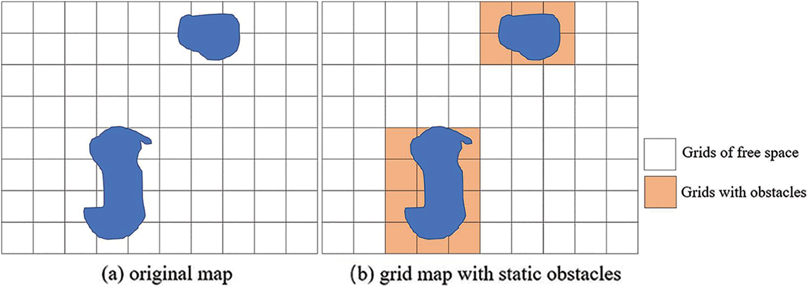
Figure 5: Static obstacles modelling

Step 3: Apply the global path planning algorithm to plan the global path.

Step 4: Compute the distance between waypoints that are directly connected to the global planning route.

2.3 Objective Function

The objective function is the core driver of local obstacle avoidance algorithms to achieve the goal. Different obstacle avoidance algorithms have different objective functions according to different metrics. For example, if the whole obstacle avoidance process takes the shortest time, the objective function takes time as the driving force [30] and evaluates how to complete obstacle avoidance in the shortest time, without considering factors such as distance or economic cost in the whole process.

In fact, if the algorithm chooses a single metric, it will lead to the obstacle avoidance process falling into local optimization or unable to complete the task. At the same time, integrating multiple objectives to design the objective function undoubtedly increases the complexity of the algorithm, and greatly reduces the real-time performance of the USV.

2.4 Communication Link

As shown in Fig. 1, the control center is the decision-making module of the USV, and command and dispatch, path planning and obstacle avoidance are the core functions of this module. The communication link layer is the intermediary between USV and control center to transmit data. This paper uses 5G technology for communication, which has the characteristics of low cost and fast transmission rate. At the same time, in order to ensure communication reliability, a redundant communication link is also provided, that is, satellite communication. The two communication links can be switched freely, satellite communication is suitable for ocean navigation environment, but the cost is relatively high.

3  Methodology

3.1 APF Algorithm

APF theory was proposed by Khatib [10] and has been applied to path planning or obstacle avoidance of robots [31], unmanned aerial vehicles [32], unmanned surface vehicles [33] and autonomous driving [34]. The artificial potential field used a virtual artificial potential field for environment modeling, which included a repulsive force and an attractive force. The target attracts the USV and guides the USV to move towards it. The obstacles repel the USV to avoid the collision between the USV and them. The total potential field of the USV environment space is the resultant force formed by the composition of the attraction field and the repulsive field, that is, the USV can complete the obstacle avoidance operation by controlling the resultant force of the two fields and reach the target smoothly. The attraction field computing method is shown as Eq. (4),

Uatt(q)=12δρ2(q,qgoal)(4)

Among them, δ is for proportion position gain coefficient, ρ(q,qgoal) is a vector, q represents the vector size and q_{goal} represents the location of waypoint, and Euclidean distance between two waypoints is |q−qgoal|. The direction of the vector is the direction of the line between the two points from the location of the USV to the target waypoint. Then the attraction force generated by the attraction field is shown as Eq. (5),

Fatt(q)=−∇Uatt(q)=δρ(q,qgoal)(5)

The repulsion force is affected by the distance between the USV and the obstacle. When the distance between the obstacle and the USV is farther, the potential energy of the obstacle is smaller, on the contrary, the potential energy of the obstacle is greater. When the USV potential energy is zero, it indicates that the USV has been out of the influence range of the obstacle, and the repulsive field function is expressed as Eq. (6),

Urep(q)={12k(1ρ(q, q0)−1ρ0)2,0≤ρ(q,q0)≤ρ00,ρ(q,q0)>ρ0(6)

where k is the proportion position gain coefficient, ρ0 is a positive constant, representing the maximum distance that the obstacle around the USV has an effect on the USV, and ρ(q,q0) represents a vector whose size is q and the closest point q0 to the USV in the obstacle around the USV, and the vector direction is the location of the obstacle pointing to the USV. Then the repulsive force generated by the repulsive field is shown as Eq. (7),

Frep(q)={k(1ρ(q, q0)−1ρ0)1ρ2(q, q0)∇ρ(q, q0),0≤ρ(q,q0)≤ρ00,ρ(q,q0)>ρ0(7)

Then, the composite potential field function can be computed as Eq. (8),

U(q)=Urep(q)+Uatt(q)(8)

The composite potential force on the USV is shown as Eq. (9),

F(q)=−∇U(q)=Frep(q)+Fatt(q)(9)

From the perspective of the potential field, the working principle of the artificial potential field method is similar to the process of moving objects from the “top of the mountain” to the “foot of the mountain”. The principle of the potential field is shown in Fig. 6.

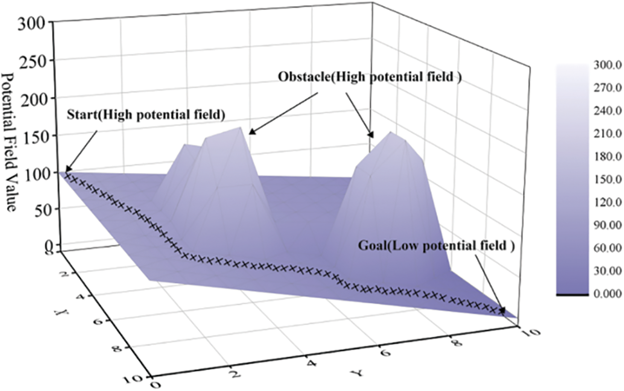
Figure 6: The principle of AFP algorithm

3.2 LSDA-APF Algorithm

The marine environment is complex and diverse, in order to solve the problem of avoiding various obstacles encountered by USV when performing tasks, we propose an improved artificial potential field obstacle avoidance algorithm to solve this problem. The USV determines the real-time coordinate position through dynamic modeling. Our proposed algorithm called local static and dynamic obstacle awareness APF algorithm (LSDA-APF). In this algorithm, the USV discrimination mechanism is used and the repulsion field function is improved to avoid the USV falling into local optimization when encountering different obstacles in different scenarios. Considering the various situations between USV and dynamic obstacles (such as vessels) during the task, the simulation results of various obstacle avoidance scenarios show that LSDA-APF algorithm can improve the local obstacle avoidance efficiency of USV.

The LSDA-APF algorithm uses the dynamic artificial potential field model, and each grid in the USV environment model has the corresponding potential field value. The USV travels along the gradient descent direction of the potential field value until it reaches the grid of the target waypoint. Considering the problem of USV falling into local optimization from the perspective of the dynamic artificial potential field, it means that when the current grid potential field value of USV is less than the surrounding grid potential field value, the USV will not select the next grid, and at this moment, USV does not reach the target waypoint, ultimately, the USV fails to find the path, and even a collision accident may occur. When the USV is trapped in local optimization and cannot make the next selection, the state value of the discrimination mechanism is true, while the default state value of the discrimination mechanism is false in the ordinary state. The calculation method of each grid value of the environment where the USV is located is shown in Eq. (10),

Uvtotal=Uvatt+∑i=1nUvrepi+Uviratt(10)

Uvtotal represents the total potential field value of each grid in the USV environment model, Uvatt represents the attraction potential field value of the target waypoint against the current grid, Uvrepi represents the repulsive potential field value of the i-th obstacle within the influence range of obstacles, n is the total number of obstacles that can affect the current grid. The total repulsive potential field value of the current grid is the sum of the repulsive potential field value of each obstacle to the grid. Uviratt is the virtual potential field. When the USV falls into the local optimization (i.e., the state value of the USV discrimination mechanism Vstatus is true), a virtual attraction potential field is dynamically added to the USV, and the grid potential field value of the current USV is increased to help the USV jump out of the local optimization area. In the ordinary state, this virtual potential field is ignored, and the value of Uviratt is 0. The calculation method of Uviratt is shown in Eq. (11),

Uviratt={12δρ2(vpre,vgoal),if vstatus=true0,else(11)

where vpre is the coordinate of the USV at the previous position and ρ(vpre, vgoal ) is the distance between the USV at the previous position and the target waypoint. At the same time, considering the situation that there may be obstacles in the USV target waypoint, the distance between the USV and the target waypoint ρ(v,vgoal) is added to the calculation of the repulsion field function to ensure that the potential field value of the target waypoint is the global minimum, and to prevent the situation that the USV cannot reach the target waypoint because of the obstacles near the target waypoint. The improved Uvrep calculation method is shown in Eq. (12),

Uvrep(v)={12η(1ρ(v,vobs)−1ρ0)2ρ2(V,vgoal),if  ρ(v,vobs)≤ρ00,ifρ(v,vobs)>ρ0(12)

When the USV jumps out of the local optimization area through the increased virtual potential field value and selects the next movable grid, the state value vstatus of the USV discrimination mechanism reverts to the default value of false. When the USV leaves the influence range of the static obstacle, that is, when the distance between the USV and the static obstacle is greater than ρ0, the USV discrimination mechanism is jumped out.

The goal of the LSDA-APF algorithm is to plan a collision-free safe route between two waypoints. LSDA-APF algorithm adopts the concept of dynamic artificial potential field, and the USV executing the task in the gradient descent direction of the total potential field until it safely avoided all obstacles and reached the target waypoint, that is, the lowest point of the whole potential field. According to the basic principle of LSDA-APF algorithm, the objective function can be obtained as shown in Eq. (13), To minimize the total potential field U, Uvatt is the attraction potential field generated by the target waypoint, n is the number of obstacles, Uvrepi is the repulsive potential field generated by obstacle i, and Uviratt is the virtual potential field.

minU=Uvatt+∑i=1nUvrepi+Uviratt(13)

The overall process of LSDA-APF obstacle avoidance algorithm is as follows:

The workflow of LSDA-APF algorithm is shown as Fig. 7.

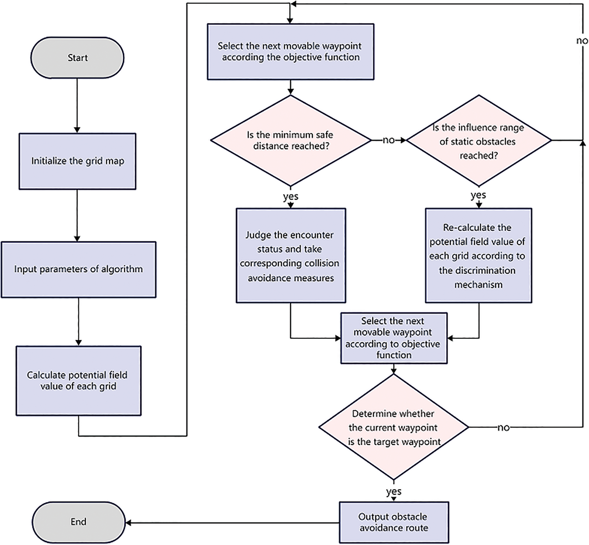
Figure 7: Flow chart of LSDA-APF algorithm

3.3 Objective Function and Cost Function

The objective function of the USV is a scheduler that performs the global path planning or the local obstacle avoidance planning, and solves the smooth switching of the state between global path planning and local obstacle avoidance. The objective function of LSDA-APF algorithm is shown as Eq. (14),

Target(x)={0, global path planning,        x≥m+v∗t1, local obstacle avoidance,   m≤x<m+v∗t (14)

When the value of objective function is 0, it means that the USV is in the global path planning state, and when the value of objective function is 1, the USV is in the local obstacle avoidance state. Where x represents the distance between the USV and the obstacle vessel ahead, m is the minimum safe distance, v is the current speed of the USV, and t is the time duration.

In this paper, the cost of USV obstacle avoidance is evaluated in two aspects, one is the economic cost, and the other is the time cost. In the case of crossing between USV and dynamic obstacle vessels, the simplest avoidance scheme is USV stopping avoidance. In this case, the economic cost of USV is the lowest. However, in the extreme case of continuous passage of dynamic obstacle vessels in front of USV, USV may fall into a standstill state and cannot continue to navigate. On the contrary, if the USV adjusts the heading angle, it increases the economic cost of navigation, which leads to the reduction of the endurance distance of the USV and the inability to reach the target. To this end, Eq. (15) is used as the cost function, and α and β are the parameters, which are both set to 1 by default.

cost=α costprice+β costtime(15)

4  Simulation and Results Analysis

In order to test the effectiveness of LSDA-APF algorithm in avoiding various obstacles, we conduct simulation experiments for USV in various obstacle scenarios. The experimental scenarios mainly include the local optimal scenario, with more static obstacles and the USV encounter scenario with fewer static obstacles. The USV encounter scenarios mainly include head-on, cross-over and over-taking scenarios.

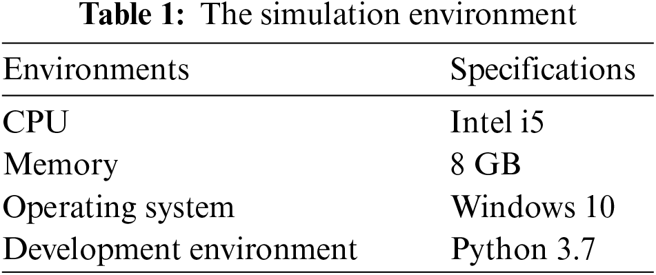
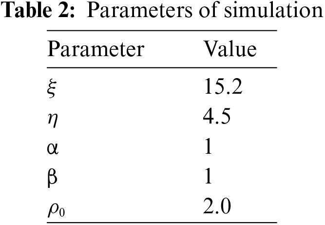
4.1 Simulation Environment and Parameter Settings

LSDA-APF algorithm is implemented using Python language. The simulation environment is shown in Table 1, and the parameters of simulation are shown in Table 2.

4.2 Simulation Results and Analysis

LSDA-APF algorithm is simulated in four different scenarios: USV trapped in the local optimization, head-on, cross-over and over-taking.

4.2.1 Trapped in the Local Optimal Scenario

When the USV sails to the area with many static obstacles such as reefs, the traditional artificial potential field obstacle avoidance algorithm easily makes the USV fall into local optimization and cannot continue to sail. In order to test the effectiveness of the LSDA-APF algorithm in solving the local optimization problem, simulations are carried out in this scenario, and the simulation scenario is shown in Fig. 8.

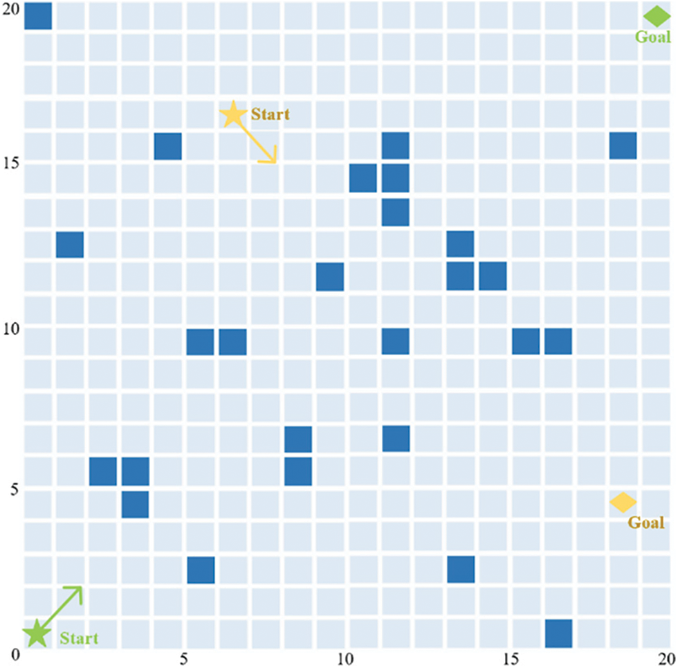
Figure 8: USV local optimization scenario

The coordinates of starting point of USV1 (represented by green track) are (0.5, 0.5), the coordinates of the ending point are (19.5, 19.5), and the speed of USV1 is 6 knots. The coordinates of starting point of USV2 (represented by yellow track) are (6.5, 16.5), the coordinates of ending point are (18.5, 4.5), the speed of USV2 is 1 knot, the time interval is 1 s, and the minimum safe distance of the USV obstacle avoidance system is 5 m.

The traditional artificial potential field method and LSDA-APF algorithm are respectively used to perform local obstacle avoidance in this scenario, and the comparison of the simulation results are shown in Figs. 9a and 9b.

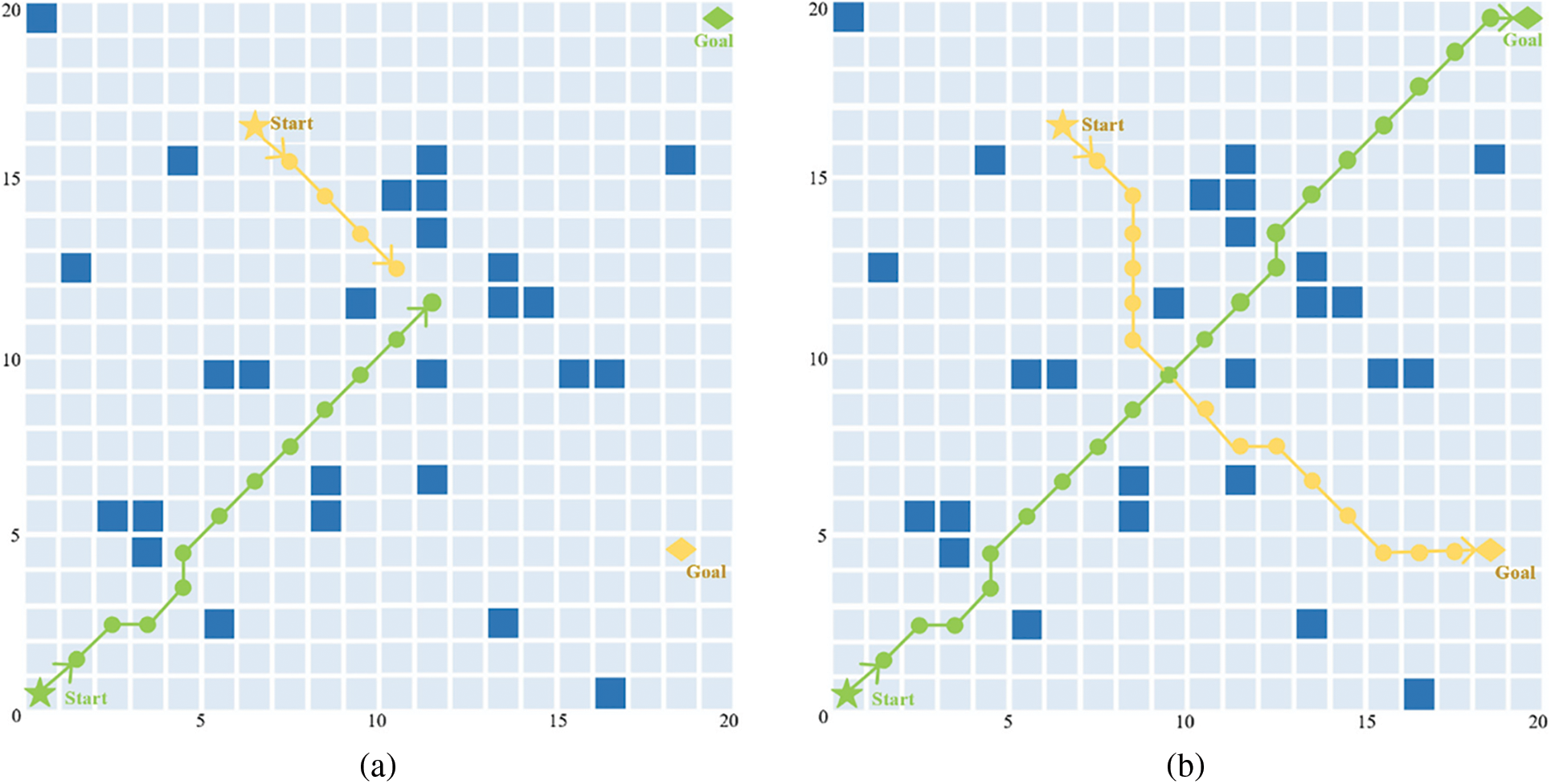
Figure 9: Comparison of navigation track in the local optimization scenario

Fig. 9a shows the obstacle avoidance simulation results of the traditional artificial potential field in the local optimization scenario of USV. The green track is the navigation route of USV1, and the yellow track is the navigation route of USV2. When USV1 runs to (11.5, 11.5) and falls into the local optimization, and the surrounding grid potential field values are larger than the grid values of USV1. As a result, USV1 cannot select the next position and stops at (11.5, 11.5). When USV2 moves to (10.5, 12.5), it also falls into the local optimization due to the influence of USV2 position, so both USV1 and USV2 fail to perform the task.

Fig. 9b shows the simulation results of LSDA-APF algorithm in the local optimization scenario of USV. When USV1 moves to (11.5, 11.5), it jumps out of the local optimal area with the help of the discrimination mechanism and selects (12.5, 12.5) as the next position. When USV2 reaches (8.5, 14.5), it enters the minimum safe distance range of the USV obstacle avoidance system. After the USV obstacle avoidance system judges that it is in the left crossing state, USV2 will adjust its course to the right to avoid USV1, and finally reach the target waypoint successfully.

4.2.2 Head-on Scenario

When two USVs are coming in opposite direction, the traditional artificial potential field obstacle avoidance algorithm cannot make the correct obstacle avoidance decision according to the current USV state. Especially when there are static obstacles such as reefs near the two USVs meeting position, the two USVs are easy to choose the same position when selecting the next lowest potential field value, which will cause a collision accident. In order to test the effectiveness of the LSDA-APF algorithm in the collision avoidance decision in the USV head-on scenario, we conduct a simulation experiment in the environment shown in Fig. 10.

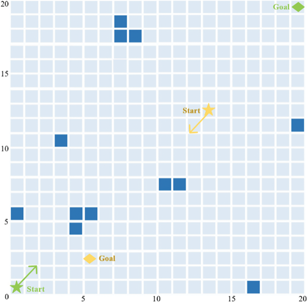
Figure 10: USV head-on scenario

The coordinates of starting point of USV1 are (0.5, 0.5), the coordinates of ending point are (19.5, 19.5), the speed is 2 knots. The coordinates of starting point of USV2 are (14.5, 12.5), the coordinates of ending point are (4.5, 2.5), the speed is 1 knot, the time step is 1 s, and the minimum safety distance of USV obstacle avoidance system is 3 m.

The traditional artificial potential field method and LSDA-APF algorithm are respectively used to perform local obstacle avoidance in the head-on scenario, and the comparison of the simulation results are shown in Fig. 11.

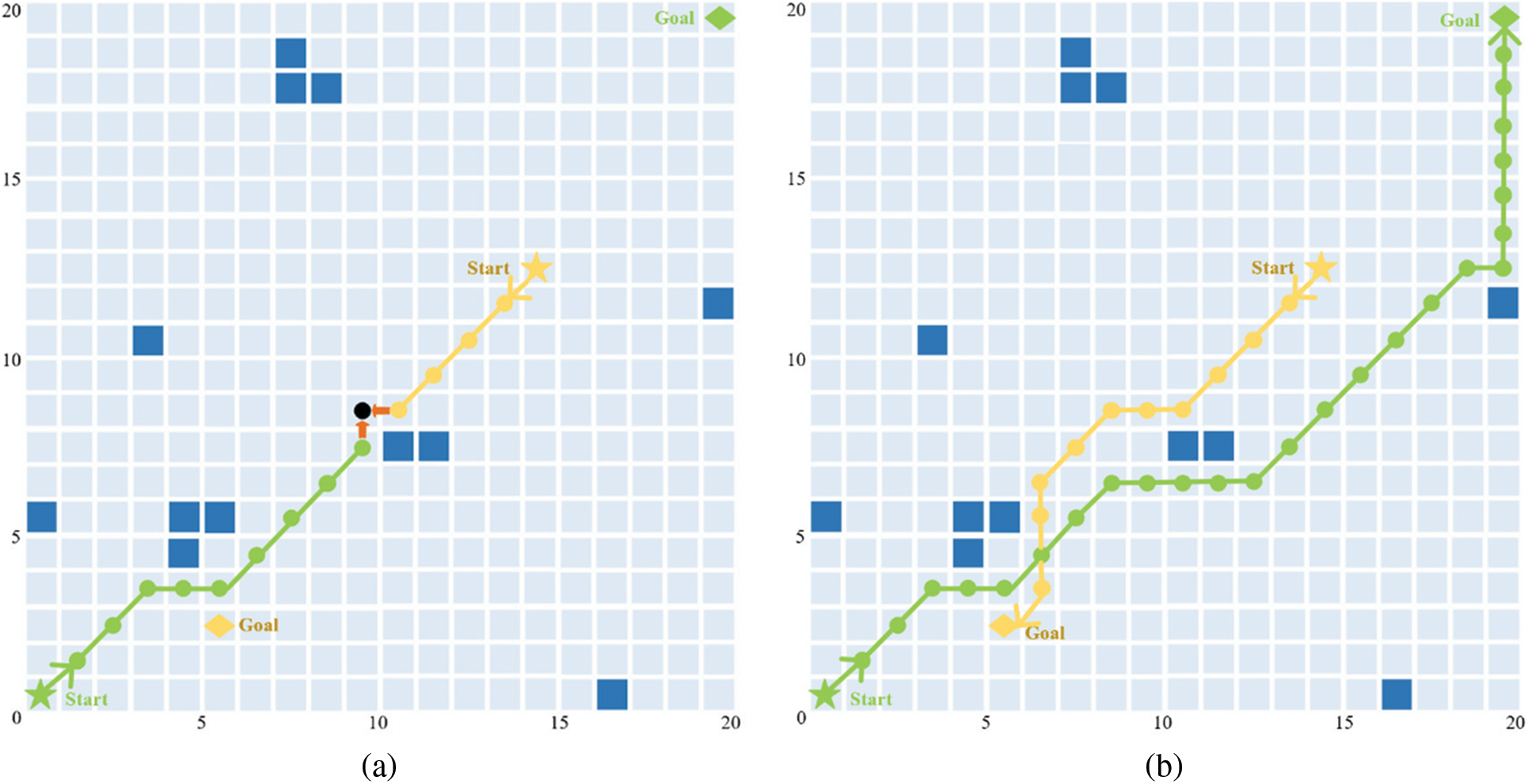
Figure 11: Comparison of navigation track in the head-on scenario

Fig. 11a shows the obstacle avoidance simulation results of the traditional artificial potential field in the USV head-on scenario, the green track is the route of USV1, and the yellow track is the route of USV2. When USV1 moves to (9.5, 7.5), the grid position of the next minimum potential field value of USV1 and USV2 is (11.5, 8.5). A collision accident occurs when USV1 and USV2 simultaneously select this position as the next moving point.

Fig. 11b shows the obstacle avoidance simulation results of LSDA-APF algorithm in the head-on scenario. When USV1 drives to (8.5, 6.5) and USV2 drives to (10.5, 8.5), USV1 reaches the minimum safe distance. After the USV obstacle avoidance system judges that it is in the head-on state, both USV1 and USV2 adjust their course to the right, and continue to drive along this course at the original speed. When USV1 reaches (12.5, 6.5), USV2 drives to (8.5, 8.5). When the distance between the two USVs is greater than the minimum safe distance, USV will jump out of the USV obstacle avoidance system, continue driving according to the objective function, and finally avoid all obstacles and reach the target waypoint smoothly.

4.2.3 Cross-over Scenario

When two USVs cross, the traditional artificial potential field obstacle avoidance cannot judge the navigation state of the dynamic obstacle while selecting the position of the minimum potential field value, and easily lead to cross-conflict accidents. We simulate this situation in the scenario shown in Fig. 12.

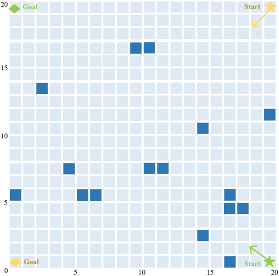
Figure 12: USV crossover scenario

The coordinates of starting point of USV1 are (19.5, 0.5) and the coordinates of ending point are (0.5, 19.5). The coordinates of starting point of USV2 are (19.5, 19.5) and the coordinates of ending point are (0.5, 0.5). The speed of both of USVs are 1 knot, the time step is 1 s, and the minimum safety distance of USV obstacle avoidance system is 2 m.

The traditional artificial potential field method and LSDA-APF algorithm are respectively used to avoid obstacles in the USV cross-over scenario, and the comparison of the simulation results are shown in Fig. 13.

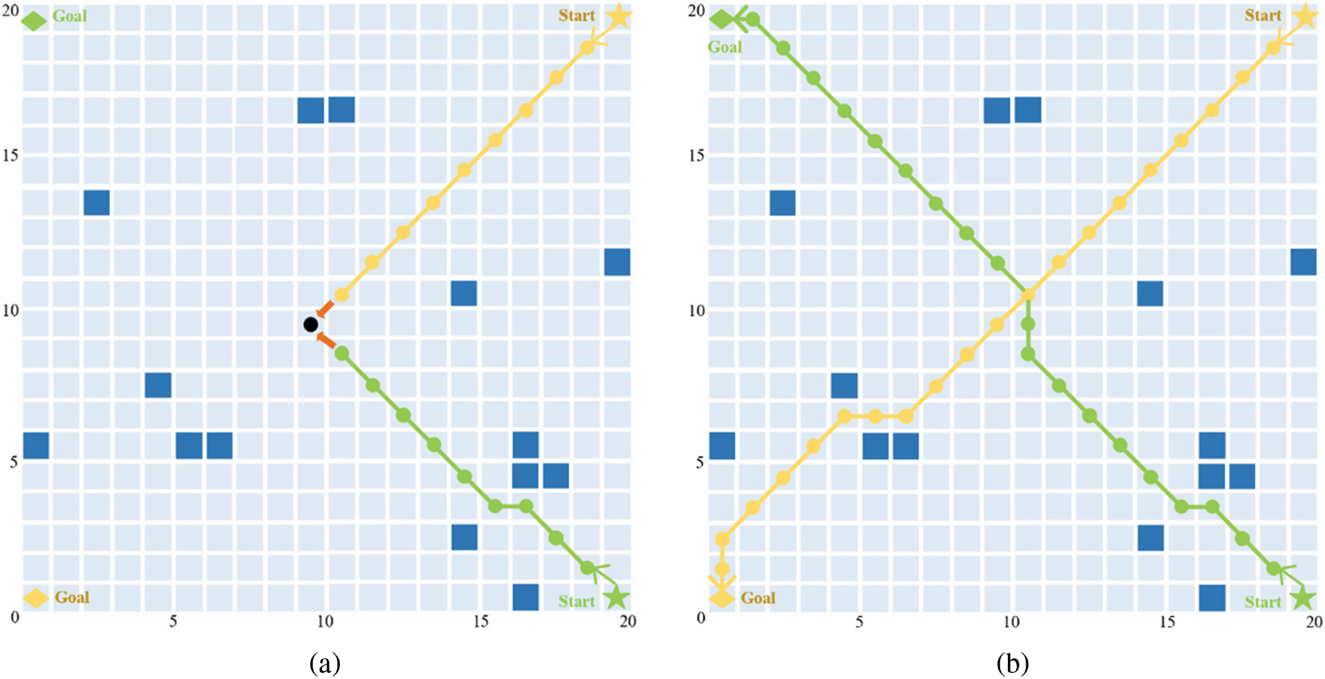
Figure 13: Comparison of navigation track in cross-over scenario

Fig. 13a shows the results of the traditional artificial potential field in the cross-over scenario. In the figure, the green track is the route of USV1, and the yellow track is the route of USV2. When USV1 moves to (10.5, 8.5), USV2 moves to (10.5, 10.5), In this case, the grid position with the smallest next potential field value of USV1 and USV2 is (9.5, 9.5), and USV1 and USV2 choose this position as the next moving point at the same time, so there is a conflict accident.

Fig. 13b shows simulation results of LSDA-APF algorithm in the cross-over scenario. When USV1 moves to (10.5, 8.5), USV2 moves to (10.5, 10.5). At this time, USV1 enters the minimum safe distance of USV obstacle avoidance system, and the USV obstacle avoidance system determines that it is a cross-right state. USV1 adjusts its course to the right and continues to move at the original speed along this course. USV2 keeps its original course and speed moving. When USV1 travels to (10.5, 10.5), USV2 travels to (8.5, 8.5), and the distance between the two USVs is greater than the safe distance, the USV obstacle avoidance system jumps out. According to the objective function, the USVs continued to drive, and finally avoided all obstacles and reached the target waypoint successfully.

4.2.4 Over-Taking Scenario

In the scenario shown in Fig. 14, when USV1 carrying out the task overtakes USV2, the traditional artificial potential field obstacle avoidance cannot make the correct obstacle avoidance decision according to the state of the USV being over-taken. When static obstacles such as rocks are encountered in the process of over-taking, if USV1 over-takes, USV2 is prone to select the same position with the lowest potential field value, the algorithm will lead to overtaking conflict accident.

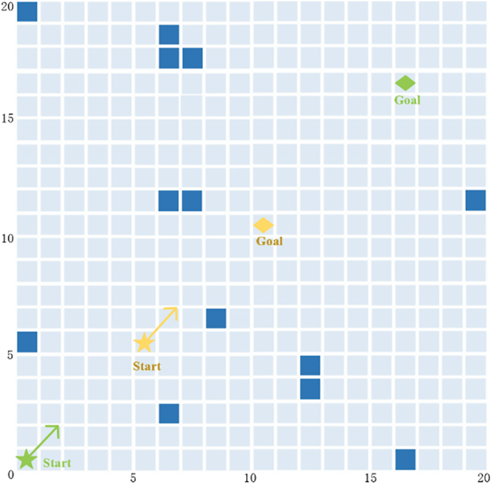
Figure 14: USV over-taking scenario

The coordinates of starting point of USV1 are (0.5, 0.5), the coordinates of ending point are (16.5, 16.5), the speed of USV1 is 4 knots, the time step is 1 s; the coordinates of starting point of USV2 are (5.5, 5.5), the coordinates of ending point are (10.5, 10.5), the speed of USV2 is 1 knot, and the minimum safety distance of USV obstacle avoidance system is 3 m.

The traditional artificial potential field method and LSDA-APF algorithm are respectively used for over-taking scenario, and the comparison of simulation results are shown in Fig. 15.

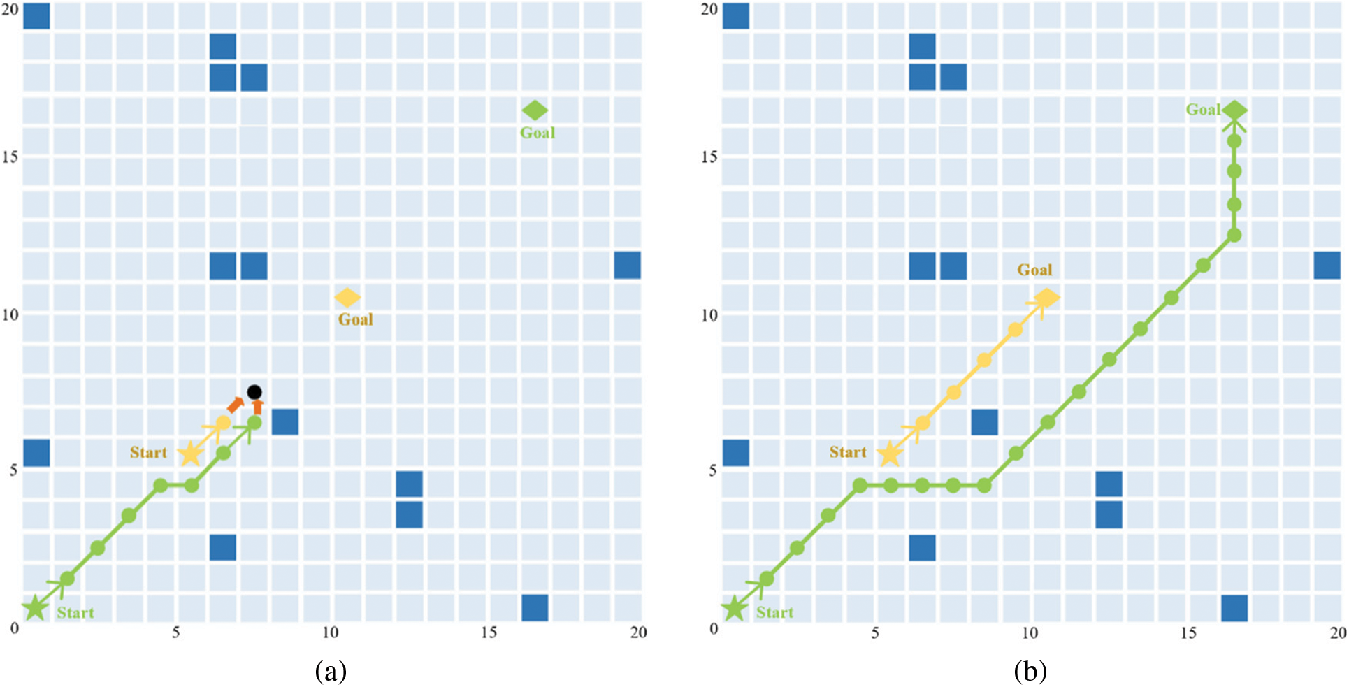
Figure 15: Comparison of navigation track in the over-taking scenario

Fig. 15a shows the simulation results of the traditional artificial potential field in the over-taking scenario. The green track in the figure is the USV1 route, and the yellow track is the USV2 route. When USV1 moves to (7.5, 6.5), the grid position of the next minimum potential field value of USV1 and USV2 are both (7.5, 7.5). A collision accident occurs when USV1 and USV2 simultaneously select this position as the next moving point.

Fig. 15b shows the simulation results of LSDA-APF algorithm in the over-taking scenario. When USV1 drives to (4.5, 4.5) and USV2 drives to (6.5, 6.5), USV1 enters the minimum safe distance of USV obstacle avoidance system, and USV obstacle avoidance system determines the over-taking state. USV1 will adjust its course to the right, and continue to drive along this course according to the original speed, USV2 will keep the original course and speed driving. When USV1 travels to (8.5, 4.5), USV2 travels to (7.5, 7.5), and the distance between the two USVs is greater than the minimum safe distance, they jump out of the USV obstacle avoidance system, and continue to drive according to the objective function. Finally, all obstacles are avoided and reach the target waypoint successfully.

4.2.5 Static Obstacles Scenario

At the same time, in order to verify the economic feasibility of the LSDA-APF algorithm in the environment of static obstacles, the algorithm and literature [35] were respectively tested for USV navigation in an environment containing multiple static obstacles. In order to solve the problem that the A* algorithm seeks a shorter path in the path search and sacrifices the smoothness of the path, the literature [35] found that the A* cost function has a significant impact on the path curve, and then introduced the artificial potential field method to improve the A* algorithm, and designed a new cost function. The improved algorithm can reduce the number of inflection points of the path, and the path is smoother. The simulation results of LSDA-APF algorithm and literature [35] are shown in Fig. 16.

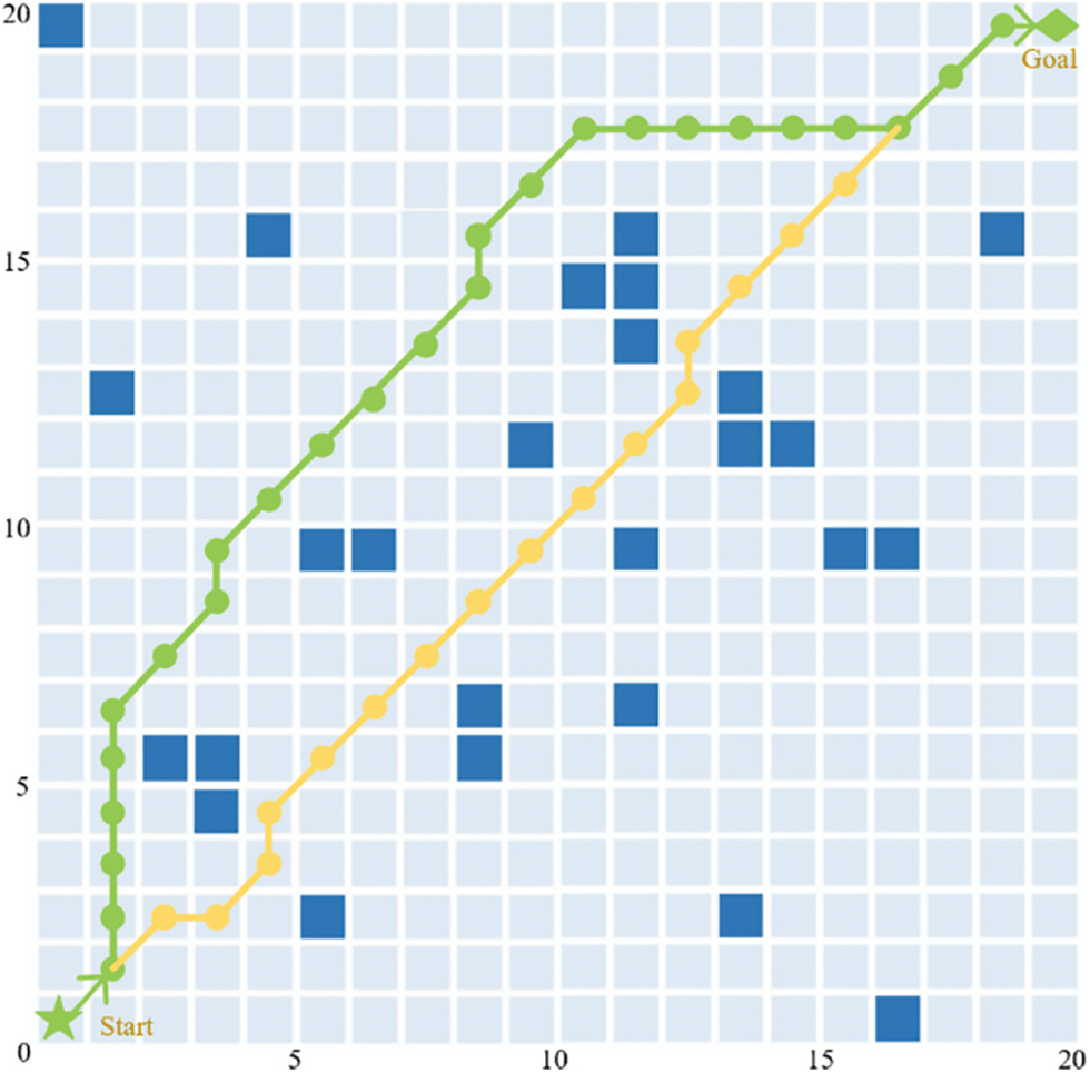
Figure 16: Comparison of navigation track in the scenario of static obstacles

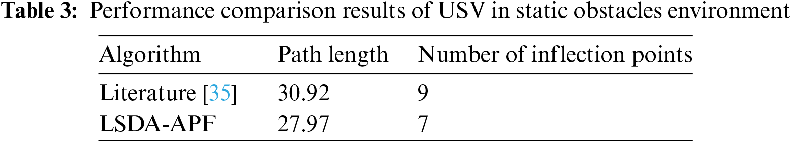
In Fig. 16, the starting point coordinates of USV are (0.5, 0.5), and the ending point coordinates are (19.5, 19.5). The green route is the obstacle avoidance route of the literature [35] algorithm, and the yellow route is the obstacle avoidance route of the LSDA-APF algorithm. It can be seen from Fig. 16 that both algorithms can avoid all static obstacles, smoothly reach the end point from the starting point, and have partially overlapping routes. From the perspective of economic feasibility, the LSDA-APF algorithm has certain advantages over the algorithm in literature [35]. The path length and inflection points are significantly reduced, which reduces the economic cost of USV. The comparison results of the specific experimental data are shown in Table 3.

The above simulation results show that the LSDA-APF algorithm can take the correct collision avoidance decision in all kinds of scenarios, and has great advantages over the traditional algorithm in the complex marine environment. Setting different safe distance threshold can reduce the distance cost while ensuring safety. It solves the problem that the traditional algorithm is easy to fall into the local optimization, overcomes the shortcomings of the traditional algorithm that is easy to make mistakes, avoids the collision accident.

5  Conclusions

Regarding the obstacle avoidance method of USV in the local marine environment, this paper proposes a local obstacle avoidance algorithm LSDA-APF with a discrimination mechanism. The algorithm is applied to the control center module of the USV system. From the architecture of the USV system, the communication link layer adopts 5G technology and satellite communication to ensure the reliability and economy of communication. In this paper, the static and dynamic obstacles in the marine environment are modeled first, and the marine environment and USV positions are represented by a grid map and 3D coordinate system. Then the LSDA-APF algorithm sets the minimum safe distance, defines the objective function and the dynamic virtual potential field mechanism, and uses the data of the distance, speed and course of the detected dynamic obstacles to effectively avoid obstacles according to the COLREGS. The simulation results show that the LSDA-APF algorithm can effectively avoid obstacles in a complex marine environment containing multiple dynamic obstacles, and better realize the state switching between local obstacle avoidance and a global path planning environment. In the static environment, the LSDA-APF algorithm is also superior to the baseline algorithm in terms of the path length and the number of inflection points, reflecting good economy and safety.

In the future, we will consider external meteorological conditions, such as the impact of wind and waves on USV steering. We will incorporate more sensor more information to ensure the stability of the USV under limited weather conditions, ensure navigation safety, and effectively avoid obstacles.

Acknowledgement: The authors are grateful for the support by the postdoctoral fund of the Science and Technology Development Fund (FDCT), Macau (Grant No. 0003/2021/APD).

Funding Statement: This work was supported by the Postdoctoral Fund of FDCT, Macau (Grant No. 0003/2021/APD). Any opinions, findings and conclusions or recommendations expressed in this material are those of the authors and do not necessarily reflect those of the sponsor.

Author Contributions: The authors confirm contribution to the paper as follows: study conception and design: Shengbin Liang; data collection: Tongtong Jiao; analysis and interpretation of the result: Xiaoli Li; draft manuscript preparation: Tongtong Jiao, Xiaoli Li; visualization: Jinfeng Ma, Dongxing Duan; methodology: Tongtong Jiao; software: Xiaoli Li, Tongtong Jiao; writting and review: Shengbin Liang.

Availability of Data and Materials: The TSPLIB data used to support the findings of this study have been deposited in the website: https://github.com/LuckyVickey/data.git.

Conflicts of Interest: The authors declare that they have no conflicts of interest to report regarding the present study.

References

1. Wang, N., Jin, X., Er, M. J. (2019). A multilayer path planner for a USV under complex marine environments. Ocean Engineering, 184, 1–10. [Google Scholar]

2. Wang, H., Xiao, P., Li, X. (2022). Channel parameter estimation of mmWave mimo system in urban traffic scene: A training channel-based method. IEEE Transactions on Intelligent Transportation Systems. [Google Scholar]

3. Raimondi, F. M., Trapanese, M., Franzitta, V., Viola, A., Colucci, A. (2015). A innovative semi-immergible USV (SI-USV) drone for marine and lakes operations with instrumental telemetry and acoustic data acquisition capability. OCEANS 2015-Genova, pp. 1–10. Genova, Italy. [Google Scholar]

4. Han, J., Cho, Y., Kim, J., Kim, J., Son, N. et al. (2020). Autonomous collision detection and avoidance for ARAGON USV: Development and field tests. Journal of Field Robotics, 37(6), 987–1002. [Google Scholar]

5. Chen, W., Hao, X., Yan, K., Lu, J., Liu, J. et al. (2021). The mobile water quality monitoring system based on low-power wide area network and unmanned surface vehicle. Wireless Communications and Mobile Computing, 2021, 1–16. [Google Scholar]

6. Xiao, X., Dufek, J., Woodbury, T., Murphy, R. (2017). Uav assisted usv visual navigation for marine mass casualty incident response. 2017 IEEE/RSJ International Conference on Intelligent Robots and Systems (IROS), pp. 6105–6110. Vancouver, Canada. [Google Scholar]

7. Wang, H., Xu, L., Yan, Z., Gulliver, T. A. (2020). Low-complexity MIMO-FBMC sparse channel parameter estimation for industrial big data communications. IEEE Transactions on Industrial Informatics, 17(5), 3422–3430. [Google Scholar]

8. Wang, H., Guo, F., Yao, H., He, S., Xu, X. (2019). Collision avoidance planning method of USV based on improved ant colony optimization algorithm. IEEE Access, 7, 52964–52975. [Google Scholar]

9. Singh, Y., Sharma, S., Sutton, R., Hatton, D., Khan, A. (2018). Feasibility study of a constrained dijkstra approach for optimal path planning of an unmanned surface vehicle in a dynamic maritime environment. 2018 IEEE International Conference on Autonomous Robot Systems and Competitions (ICARSC), pp. 117–122. Terres Vedras, Portugal. [Google Scholar]

10. Khatib, O. (1986). The potential field approach and operational space formulation in robot control. Adaptive and Learning Systems: Theory and Applications, pp. 367–377. Boston, USA. [Google Scholar]

11. Fox, D., Burgard, W., Thrun, S. (1997). The dynamic window approach to collision avoidance. IEEE Robotics & Automation Magazine, 4(1), 23–33. [Google Scholar]

12. Fiorini, P., Shiller, Z. (1998). Motion planning in dynamic environments using velocity obstacles. The International Journal of Robotics Research, 17(7), 760–772. [Google Scholar]

13. Borenstein, J., Koren, Y. (1991). The vector field histogram-fast obstacle avoidance for mobile robots. IEEE Transactions on Robotics and Automation, 7(3), 278–288. [Google Scholar]

14. Lyu, H., Yin, Y. (2017). Ship’s trajectory planning for collision avoidance at sea based on modified artificial potential field. 2017 2nd International Conference on Robotics and Automation Engineering (ICRAE), pp. 351–357. Shanghai, China. [Google Scholar]

15. Song, A., Su, B., Dong, C., Shen, D., Xiang, E. et al. (2018). A two-level dynamic obstacle avoidance algorithm for unmanned surface vehicles. Ocean Engineering, 170, 351–360. [Google Scholar]

16. Fan, X., Guo, Y., Liu, H., Wei, B., Lyu, W. (2020). Improved artificial potential field method applied for AUV path planning. Mathematical Problems in Engineering, 2020, 1–21. [Google Scholar]

17. Ren, J., Zhang, J., Cui, Y. (2021). Autonomous obstacle avoidance algorithm for unmanned surface vehicles based on an improved velocity obstacle method. ISPRS International Journal of Geo-Information, 10(9), 618. [Google Scholar]

18. Kuwata, Y., Wolf, M. T., Zarzhitsky, D., Huntsberger, T. L. (2013). Safe maritime autonomous navigation with COLREGS, using velocity obstacles. IEEE Journal of Oceanic Engineering, 39(1), 110–119. [Google Scholar]

19. Wang, J., Wang, R., Lu, D., Zhou, H., Tao, T. (2022). USV dynamic accurate obstacle avoidance based on improved velocity obstacle method. Electronics, 11(17), 2720. [Google Scholar]

20. Xia, G., Han, Z., Zhao, B., Wang, X. (2020). Local path planning for unmanned surface vehicle collision avoidance based on modified quantum particle swarm optimization. Complexity, 2020, 1–15. [Google Scholar]

21. Zhou, Y., Dong, L. (2022). Time-consuming calculation and simulation of unmanned surface vessel (USV) steering based on dynamic window approach (DWA). Proceedings of the 2022 2nd International Conference on Control and Intelligent Robotics, pp. 181–185. Nanjing, China. [Google Scholar]

22. Zhang, J., Zhao, H., Wang, N., Guo, C. (2021). Fuzzy dual-window DWA algorithm for USV in dense obstacle conditions. Chinese Journal of Ship Research, 16(6), 10–18. [Google Scholar]

23. Ni, H., Guan, W., Wu, C. (2020). USV obstacle avoidance based on improved watershed and VFH method. 2020 11th International Conference on Prognostics and System Health Management (PHM-2020 Jinan), pp. 543–546. Jinan, China. [Google Scholar]

24. Wu, C., Wang, Y., Ma, L., Rakić, A. (2021). VFH+ based local path planning for unmanned surface vehicles. 2021 IEEE International Conference on Recent Advances in Systems Science and Engineering (RASSE), pp. 1–6. Shanghai, China. [Google Scholar]

25. Zhang, G., Zhang, Y., Xu, J., Chen, T., Zhang, W. et al. (2022). Intelligent vector field histogram based collision avoidance method for AUV. Ocean Engineering, 264, 112525. [Google Scholar]

26. Corchado, E., Mata, A., Baruque, B., Corchado, J. M., Pérez-Lancho, B. (2011). A Topology-preserving system for environmental models forecasting. International Journal of Computer Mathematics, 88(9), 1979–1989. [Google Scholar]

27. Garrido, S., Moreno, L., Abderrahim, M., Martin, F. (2006). Path planning for mobile robot navigation using voronoi diagram and fast marching. 2006 IEEE/RSJ International Conference on Intelligent Robots and Systems, pp. 2376–2381. Beijing, China. [Google Scholar]

28. Khodade, P., Malhotra, S., Kumar, N., Iyengar, M. S., Balakrishnan, N. et al. (2007). Cytoview: Development of a cell modelling framework. Journal of Biosciences, 32, 965–977. [Google Scholar] [PubMed]

29. Kim, S., Jang, H., Cha, Y., Yu, H., Lee, S. et al. (2020). Development of a ship route decision-making algorithm based on a real number grid method. Applied Ocean Research, 101, 102230. [Google Scholar]

30. Kazim, I., Tan, Y., Qaseer, L. (2021). Integration of DE algorithm with PDC-APF for enhancement of contour path planning of a universal robot. Applied Sciences, 11(14), 6532. [Google Scholar]

31. Huang, T., Huang, D., Qin, N., Li, Y. (2021). Path planning and control of a quadrotor UAV based on an improved APF using parallel search. International Journal of Aerospace Engineering, 2021, 1–14. [Google Scholar]

32. Chen, Y., Luo, G., Mei, Y., Yu, J., Su, X. (2016). UAV path planning using artificial potential field method updated by optimal control theory. International Journal of Systems Science, 47(6), 1407–1420. [Google Scholar]

33. Zhang, G., Han, J., Li, J., Zhang, X. (2022). APF-based intelligent navigation approach for USV in presence of mixed potential directions: Guidance and control design. Ocean Engineering, 260, 111972. [Google Scholar]

34. Fang, Y., Wang, S., Bi, Q., Wu, G., Guan, W. et al. (2022). Research on path planning and trajectory tracking of an unmanned electric shovel based on improved APF and preview deviation fuzzy control. Machines, 10(8), 707. [Google Scholar]

35. Tian, Z., Han, X., Tian, S., Wang, J. (2022). Research on intelligent wheelchair path planning based on improved A* algorithm. Journal of Tianjin University of Science & Technology, 37(5), 38–43. [Google Scholar]