An Interpolation Method for Karhunen–Loève Expansion of Random Field Discretization

1  Introduction

In civil engineering, it is commonplace for the material properties and geometric dimensions of structures to exhibit inherent uncertainties. In the context of engineering systems, it is imperative to consider the presence of uncertainties during the analysis and design phase. These uncertainties are commonly attributed to the random spatial variation of certain properties. Traditional approaches that rely on simulating the characteristics of random structures with single random variables are deemed insufficient, as they fail to account for point-to-point variability [1]. An alternative mathematical model that has gained significant traction in the field is the continuous random field model, which accurately captures the spatial variation of a structure’s properties. Specifically, a random field is a stochastic process defined on a continuous region, where each point is associated with a random variable. However, the computation of the entire random field is unfeasible due to the infinite number of random variables involved. To facilitate the calculations, a limited number of random variables must be applied to represent the random field, which is referred to as random field discretization [2].

The methods used for random field discretization can be broadly categorized into two types: spatial discretization and series expansion. Spatial discretization methods comprise the central point method [3], the local mean method [4], the shape function method [5], and the optimal linear estimation method [6]. Among these, the local average method is commonly used due to its stable calculation results and insensitivity to the structures associated with the random field. The efficiency and accuracy of the spatial discretization methods are closely related to the random field mesh.

Series expansion methods used for random field discretization include Karhunen–Loève (KL) expansion [7,8], orthogonal polynomial expansion [9], etc. The KL expansion, introduced by Ghanem et al. [10], has emerged as the most extensively applied series expansion method for random field discretization, particularly in the context of uncertainties related to input parameters [11]. Moreover, when considering the global mean square error with respect to the number of random variables, the KL expansion is optimal compared to other series expansion methods [10]. KL expansion uses a linear combination of orthogonal bases to represent random fields, and the selected orthogonal functions are the eigenfunctions of the Fredholm integral equation of the second kind. The integral kernel function in the Fredholm integral equation is the covariance function of the random field. For simple geometries and special covariance functions, analytical solutions can be obtained. However, for more general scenarios, numerical methods are required to solve a Fredholm integral eigenvalue problem (IEVP), with the Galerkin method being the most commonly used [2].

In one-dimensional domains, the Galerkin method is frequently employed in a spectral sense with basis functions spanning over the entire domain. The convergence behavior of this approach is examined in [12] for both stationary and non-stationary problems using polynomials with order up to ten as basis functions. Other polynomial bases, such as Legendre polynomials [9], Gegenbauer polynomials [13], and Chebyshev polynomials [14], have also been proposed. However, these methods can only improve the calculation accuracy by increasing the polynomial order, which requires significant computational effort. The wavelet-Galerkin method [15] also represents a Galerkin-based technique for solving Fredholm integral eigenvalue problems in one-dimensional domains. For two-dimensional and three-dimensional domains with random fields, Ghanem et al. [10] advocated using the finite element method (FEM) to obtain approximate solutions for the KL expansion, while Papaioannou [13] examined the convergence of the FEM in two-dimensional domains. Based FEM-Galerkin method for the discretization of the IEVP, Allaix et al. [1] proposed a genetic algorithm to achieve an optimal discretization of 2D homogeneous random fields. To compute matrix eigenvalue problems in the FEM, a generalized fast multi-pole Krylov eigen-solver is employed [16]. In two-dimensional and particularly three-dimensional random fields, the computational cost of constructing the matrix eigenvalue problem and computing its solution can be prohibitively expensive. Basmaji et al. [17] proposed a Galerkin scheme based on discontinuous Legendre polynomials to solve IEVP, which reduces the computational complexity by constructing the Legendre basis on each local element domain and exploiting the orthogonality of Legendre polynomials. In addition, generating meshes for complex geometries may also present difficulties and time constraints. To circumvent this issue, Rahman et al. [18] employed meshless basis functions in the Galerkin method for complex domains. Papaioannou [13] introduced a spectral Galerkin method that addresses the challenges posed by geometrically complex domains by embedding the actual domain into a simple geometric shape. Rahman [19] proposed the Galerkin isogeometric method for KL approximation which can denote computational domains by non-uniform rational B-splines(NURBS).

The development of a method that can efficiently solve the IEVP with reduced computational requirements and without the need for a complex mesh is crucial for effectively addressing complex domain problems. In this study, an interpolation approach for solving the IEVP in KL expansion is proposed. And the impact of three different interpolation basis functions, namely moving least squares [20–22] (MLS), least squares [23] (LS), and finite element method (FEM), on the accuracy of computation is explored. MLS and LS are widely used in meshless methods [22,24–26]. The results demonstrate that for one-dimensional domains, the proposed interpolation method, which requires a single integral for the integral matrix containing the covariance function, is more computationally efficient than the Galerkin method, which requires a two-folded integral.

In addition, we employ a combination of KL expansion and polynomial chaos expansion to perform stochastic analysis in two-dimensional domains. To tackle the issue of grid division in irregular domains, we introduce the extended finite element method (XFEM) as an alternative to the traditional finite element method. The XFEM [27,28] is a well-known numerical method that addresses discontinuity problems based on the partition of unity theory [29]. This approach adds enrichment functions to the displacement mode of conventional finite element methods to accurately represent discontinuities. The key advantage of the XFEM is that the computational mesh is independent of the internal geometry or physical interface of the structure, making it an effective method for solving problems that involve discontinuities, especially in the presence of holes [30].

The structure of this paper is as follows: Section 2 introduces the KL expansion and its fundamental properties. Additionally, the numerical methods used to solve IEVP, namely the Galerkin method and the interpolation method, are discussed. Interpolation basis functions such as MLS, LS, and FEM are provided. Section 3 briefly describes the spectral stochastic finite element method and extended finite element method, which are then used for stochastic analysis of complex domains. Section 4 is dedicated to numerical examples, wherein the computational efficiency of the numerical methods is compared in one-dimensional domains, and the stochastic analysis is conducted in both 2D regular and irregular domains. The benefits of the proposed method are highlighted. At last, Section 5 concludes the paper.

2  Karhunen–Loève Expansion

Defining (Θ,ℱ,P) is a complete probability space, Θ is the sample space. A continuous random field H(x,θ) is a measurable function H:Ω×Θ→R indexed by the space coordinates x∈Ω∈Rn, where Ω is a continuously bounded domain. For a given x0∈Ω, H(x0,θ) is a random variable. For a given outcome θ0∈Θ,H(x,θ0) is a realization of the field. In practice, it is difficult to apply a continuous random field directly, so the random field needs to be treated with discretization. Karhunen–Loève expansion is a series expansion method for representing the random field. which is founded upon the spectral decomposition of the field's covariance function. The Karhunen–Loève expansion of a second-order random field can be expressed as [10]

H(x,θ)=μ(x)+∑i=1∞λiϕi(x)ξi(θ)(1)

where μ(x) is the mean function, ξi(θ) are standard uncorrelated random variables, i.e., E[ξi(θ)]=0,E[ξi(θ)ξj(θ)]=δij. λi and ϕi are the eigenvalues and eigenfunctions of the covariance function respectively which can be obtained from solving the homogeneous Fredholm integral equation of the second kind:

∫ΩCov(x,x′)ϕ(x′)dΩx′=λiϕi(x)(2)

where Cov(x,x′) is the covariance function which can be represented as Cov(x,x′)= σ(x)⋅σ(x′)⋅ρ(x,x′), σ is the standard deviation function of the random field and ρ is the correlation function. Cov(x,x′) is also called as kernel function, and it is bounded, symmetric and positive semi-definite [4].

According to Mercer’s Theorem [31], the eigen-decomposition of the covariance function is as follows:

Cov(x,x′)=∑i=1∞λiϕi(x)ϕi(x′)(3)

The eigenvalues λi are nonnegative, and the eigenfunctions ϕi(x) form a completely orthogonal set satisfying the following equation:

∫Ωϕi(x)ϕj(x′)dΩ=δij(4)

where δij is the Kronecker-delta function.

Due to the orthogonality of eigenfunctions, it is easy to get a closed form of each random variable as follows:

ξi(θ)=1λi∫Ω[H(x,θ)−μ(x)]ϕ(x)dΩ(5)

In the case where the random field H(x,θ) is Gaussian, the ξi are independent standard normal random variables [10]. The joint distribution of ξi is almost impossible to acquire in other cases. However, scholars have also studied the non-Gaussian random process simulation based on KL expansion. Phoon et al. [32] developed an iterative framework to simulate non-stationary and non-Gaussian processes. Sakamoto et al. [33] used the polynomial chaos expansion of a Gaussian stochastic process to represent the non-Gaussian process, while the Gaussian stochastic process is modeled by the KL expansion. Dai et al. [34] used the one-dimensional polynomial chaos expansion to decompose the random coefficients in the KL expansion and obtained the explicit representation of non-Gaussian and non-stationary random processes described by the covariance function and the marginal cumulative distribution function which is suitable for random finite element analysis of structures. Tong et al. [35] combined Karhunen–Loève expansion with the Linear-moments-based (L-moments-based) Hermite polynomial model for simulating strongly non-Gaussian and non-stationary processes.

For practical implementation, the random field H(x,θ) can be acquired through sorting the eigenvalues λi in a descending order and truncating the series expansion at the M-th term

H~(x,θ)=μ(x)+∑i=1Mλiϕi(x)ξi(θ)(6)

The second-order statistics of the truncated series Eq. (6) can be presented as

Cov[H~(x,θ),H~(x′,θ)]=E{[H~(x,θ)−μ(x)][H~(x′,θ)−μ(x′)]}=∑i=1M∑j=1Mλiλjϕi(x)ϕj(x)E[ξi(θ)ξj(θ)]=∑i=1Mλiϕi(x)ϕj(x′)(7)

As M→∞, Eq. (7) converges to Eq. (3). The variance function of the approximated random field is

Var[H~(x,θ)]=∑i=1Mλiϕi2(x)(8)

The error ϵH~ between the original random field H(x,θ) and its approximate random field H~(x,θ) is

ϵH~,M(x,θ)=H(x,θ)−H~(x,θ)(9)

Integration of the expectation of the squared approximation error over the domain Ω yields the global mean square error [10]

ϵ¯H2=∫ΩE[(ϵH~,M(x,θ))2]dx(10)

An alternative error estimation is the error variance [6] which is defined as follows:

ϵVar,M(x)=Var[H(x,θ)−H~(x,θ)]Var[H(x,θ)]=σ2(x)−∑i=1Mλiϕi2(x)σ2(x)(11)

The corresponding mean error variance is given as

ϵ¯Var,M=1|Ω|∫ΩϵϵVar,Mdx=1−1|Ω|∑i=1Mλi∫Ωϕi2(x)σ2(x)dx(12)

where |Ω|=∫Ωdx.

If the variance of the random field is constant, i.e., ∀x∈Ω,σ(x)=σ, the mean error variance ϵ¯Var,M can be reduced to

ϵ¯Var,M=1−1|Ω|σ2∑i=1Mλi(13)

The error variance in this section is based on the analytical solutions of eigenvalues and eigenfunctions. However, it is not always possible to obtain the analytical eigen-solutions in practical engineering applications. Therefore, in the following sections, we will introduce other error measures in the numerical examples to evaluate the accuracy of the proposed interpolation method.

2.1 Numerical Solution of the Fredholm Integral Equation

The key to KL expansion is to find the eigenvalues and eigenfunctions of the covariance function by solving a Fredholm integral eigenvalue problem of Eq. (2). The analytic solution of Eq. (2) is only applicable to a finite set of covariance functions and geometric domains. For general cases, the numerical method is the only recourse. Therefore, the random field approximation of truncated KL expansion in Eq. (6) can be approximated as

H~(x,θ)=μ(x)+∑i=1Mλ^iϕ^i(x)ξ^i(θ)(14)

where λ^i and ϕ^i are the approximate values of the true eigenvalues λi and eigenfunctions ϕi, respectively. And ξ^i are standard uncorrelated random variables.

2.1.1 The Galerkin Method for Fredholm Integral Equation

Let {hk(x)} be a complete basis of the Hilbert space ℒ2(Ω). In the Galerkin method, the eigenfunction ϕ^i(x) can be reprsented over the basis as

ϕ^i(x)=∑k=1Ndkihk(x)(15)

where dki are the coefficients of the i-th eigenfunction.

Substituting Eq. (15) into Eq. (2) and adopting a Galerkin procedure for the corresponding residual, the equation is obtained as follows:

∑k=1Ndki[∫Ω∫ΩCov(x,x′)hk(x)hl(x′)dxdx′]−λi∑k=1Ndki[∫Ωhk(x)hl(x)dx]=0(16)

Eq. (16) could rewritten as

CD=ΛGD(17)

where

Clk=∫Ω∫ΩCov(x,x′)hk(x)hl(x′)dxdx′(18)

Dki=dki(19)

Λil=δilλl(i,l=1,…,N)(20)

Glk=∫Ωhk(x)hl(x)d(21)

The eigenvalues λi exists in the diagonal of matrix Λ. By solving the generalized matrix eigenvalue problem of Eq. (17), the approximate eigenvalue λ^i and the coefficients of basis function dki are obtained. Substituting dki to Eq. (15) can get approximate eigenfunctions ϕ^i(x).

Various types of basis functions can be utilized with the Galerkin method, including orthogonal polynomials such as Legendre polynomials, which yield a diagonal matrix G. However, increasing the order of these polynomials is the only way to enhance the accuracy of the approximation, and this can lead to numerical issues if the correlation length of the random field is too small. Another frequently used basis function is the shape function of the finite element method, also known as the FEM-based Galerkin method [2]. However, this method requires domain Ω meshing, which can be a challenging task for complex geometries. Moreover, the computation of the matrix C can be time-consuming, particularly in two and three dimensions.

2.1.2 The Interpolation Method for Fredholm Integral Equation

In the random field discretization based on KL expansion, it is necessary to integrate all the elements in matrix C by using the Galerkin method to solve IEVP. In the case of a one-dimensional domain, the elements in C involve a double integral, whereas for a two-dimensional domain, a four-folded integral is required. As the dimensionality of the problem increases, the computational cost escalates significantly. To address this issue, we propose an interpolation method for solving the IEVP of Eq. (2) which is a homogeneous Fredholm integral equation of the second kind. To better illustrate the computing process of the proposed interpolation method, we start with the general form of the Fredholm integral equation of the second kind,

P(x)m(x)=Q(x)∫abL(x,x′)m(x′)dx′+f(x)(22)

where P(x),Q(x),f(x) are continuous functions on the interval [a,b], and P(x)≠0. The integral kernel function L(x,x′) is a continuous function of two variables on the interval [a,b]×[a,b].

The key problem of the Fredholm integral equation is the discretization of unknown functions. Firstly, the integral interval [a,b] is discretized as a=x1<x2<⋯<xn=b, n is the number of nodes. m1,m2,…,mn are the corresponding function values of nodes. Then the approximating function m(x) can be expressed as

m(x)=∑I=1nNI(x)mI(23)

where NI(x) is the basis function of interpolation, and I is the node of interpolation.

Substituting Eq. (23) into Eq. (22), and let the equation be true at the nodes xJ(J= 1,2,…,n), one can obtain

P(xJ)∑I=1nNI(xJ)mI=Q(xJ)∫abL(xJ,x′)∑I=1nNI(x′)mIdx′+f(xJ)J=1,2,…,n(24)

Switching the order of integration and summating the integral term of right-hand side of Eq. (24) yield

Q(xJ)∫abL(xJ,x′)∑I=1nNI(x′)mIdx′=Q(xJ)∫ab(∑I=1nL(xJ,x′)NI(x′)mI)dx′=Q(xJ)∑I=1n(∫abL(xJ,x′)NI(x′)dx′)mI=Q(xJ)∑I=1nLI(xJ)mI(25)

where

LI(xJ)=∫abL(xJ,x′)NI(x′)dx′I,J=1,2,…,n(26)

Eq. (24) is rewritten as

P(xJ)∑I=1nNI(xJ)mI=Q(xJ)∑I=1nLI(xJ)mI+f(xJ)(27)

If I=J,NI(xJ)=1,I≠J,NI(xJ)=0, Eq. (27) can be presented in a matrix form as

(P−QL)m=f(28)

where

P=diag(P(xJ))=[P(x1)⋱P(xn)](29)

Q=diag(Q(xJ))=[Q(x1)⋱Q(xn)](30)

L=[LI(xJ)]n×n(31)

m={m1,m2,…,mn}T(32)

Comparing Eqs. (2) and (22), we can see that f(x)=0, Q is a identity matrix and P=λI. Therefore, Eq. (28) can be converted into the following form:

(λI−QL)m=0(33)

By solving the eigenvalue problem of Eq. (33), the approximate eigenvalues λ^ and the corresponding node values m can be calculated. The eigenfunctions can be obtained by substituting m into Eq. (23).

Compared with the Galerkin method, which requires a two-folded integral to calculate the elements of matrix C in one dimension, the interpolation method only requires a single integral to calculate the elements of matrix L. Obviously, interpolation method needs less computation.

The selection of the basis function is a crucial step in interpolation methods. This paper discusses three choices of basis functions, namely moving least squares [20–22] (MLS), least squares [23] (LS), and finite element method (FEM). The MLS is primarily introduced, and the LS can be derived from it. Although the finite element method is not discussed in detail in this paper, it is another viable option for basis functions.

If the domain Ω discretes into n nodes and the values of eigenfunction at the nodes xI are known. The approximate eigenfunction ϕ^(x) using moving least squares interpolation can be written as follows:

ϕ^(x)=mh(x)=∑i=1tpi(x)ai(x)=pT(x)a(x)(34)

where t is the number of terms in the basis, p(x) is a polynomial basis, a(x) is the vector of coefficients, which are functions of the spatial coordinates x. For 1D problems, commonly used bases are p=[1,x]T for t=2 and p=[1,x,x2]T for t=3, etc. In the same way, for 2D problems, generally used bases are p=[1,x,y]T for t=3 and p=[1,x,y,x2,xy,y2]T for t=6, etc.

The weighted square sum of error of function m(x) at nodes is

J(x)=∑I=1nwI(x)[∑i=1tpi(xI)ai(x)−mI]2(35)

where mI=m(xI) are the values of function at node xI,wI(x) is a weight function that is greater than zero only in a finite domiam ΩI around node x, and it is zero outside of ΩI, as shown in Fig. 1. wI(x) is compactly supported and ΩI is the support domain. A typical choice for wI(x) is the normalized Gaussian function, namely

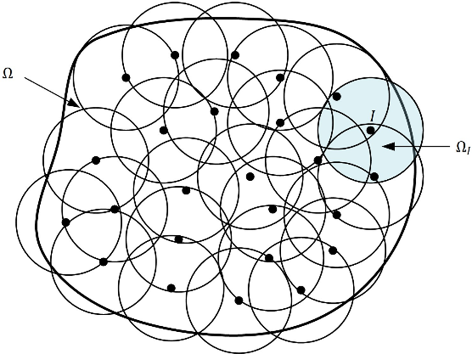
Figure 1: The support domains of nodes

wI(r)={e−r2β2−e−β21−e−β2r≤10r>1(36)

where β is a constant, r=∥x−xI∥/dmI, and dmI=ds×cI is the radius of the support domain of point xI,ds is the multiplier greater than 1 , and cI is the distance between the node xI and its nearest node.

Minimizing the weighted square sum of error J, namely

∂J∂aj(x)=2∑I=1nwI(x)[∑i=1tpi(xI)ai(x)−mI]pj(xI)=0j=1,2,…,m(37)

Then it leads to

A(x)a(x)=B(x)m(38)

where

A(x)=∑I=1nwI(x)p(xI)pT(xI)(39)

B(x)=[w1(x)p(x1),w2(x)p(x2),…,wn(x)p(xn)](40)

m=[m1,m2,…,mn]T(41)

The vector a(x) can be obtained from Eq. (38), and substituting it into Eq. (34). Then the shape function of moving least squares can be obtained as

N(x)=pT(x)A−1(x)B(x)(42)

In the process, if the weight function ωI(x) is equal to

ωI(x)={1∀x∈ΩI0∀x∉ΩI(43)

The moving least squares is reduced to least squares (LS), and matrix A of Eq. (39) and matrix B of Eq. (40) become

A(x)=∑I=1np(xI)pT(xI)(44)

B(x)=[p(x1),p(x2),…,p(xn)](45)

3  The Stochastic Analysis

In this section, we first describe the theoretical formulation of the spectral stochastic finite element method which is a numerical approach to model the random parameter system in terms of finite element framework. While, for the irregular domains, we applied the extended finite element method instead of the finite element method for calculation. It is well-known that the extended finite element method (XFEM) is an effective numerical method for solving discontinuity problems [27,28]. Based on the partition of unity method [29], XFEM adds some enrichment functions into the displacement mode of the finite element method to reflect discontinuity, and it has the advantage that the mesh is independent of the geometry or physical interface inside the structure. Therefore, for random analysis of irregular domains, XFEM has more advantages. Moreover, the basis function of XFEM can also be used as the basis function of the interpolation method to solve a Fredholm integral eigenvalue problem in KL expansion.

The spectral stochastic finite element method introduced by Ghanem et al. [10] is an extension of the deterministic finite element method for solving boundary value problems of stochastic material properties. It supposes that the material Young’s modulus is a Gaussian random field. The elasticity matrix in point x is written as

D=H(x,θ)D0(46)

where D0 represents a constant matrix.

Applying the KL expansion in Eq. (1), the stochastic matrix of a finite element has the following form:

ke(θ)=k0e+∑i=1∞kieξi(θ)(47)

where k0e is the mean element stiffness matrix, kie are deterministic matrices given by

kie(θ)=λi∫Ωeϕi(x)BTD0BdΩe(48)

where B is the strain-displacement matrix.

Assuming that the loading is determined and denoting ξ0(θ)=1, the finite element equilibrium equation is

(∑i=0∞Kiξi(θ))u(θ)=F(49)

where thee nodal displacement vector u is presented by polynomial chaos expansion (PCE) as follows:

u(θ)=∑j=0∞ujΨj(θ)(50)

where {Ψj(ξ)}j∞ are Hermite polynomial chaos.

Substituting the expansion Eq. (50) into Eq. (49) yields:

(∑i=0∞Kiξ(θ))(∑j=0∞ujΨ(θ))=F(51)

For calculating purposes, truncating the KL expansion after M terms and polynomial chaos expansion after P terms results in

ϵM,P=(∑i=0MKiξ(θ))(∑j=0P−1ujΨ(θ))−F(52)

where P=(p+M)!/(p!M!), p is the order of polynomial chaos.

By making the residual orthogonal to the approximate space spanned by PCE, one can get

∑i=0M∑j=0P−1cijkKiuj=Fkk=0,…,P−1(53)

where cijk=E(ξiΨjΨk), and Fk=E(ΨkF). E(⋅) denotes the mathematical expectation.

Eq. (53) can be rewritten as

[K0,0K0,1⋯K0,P−1K1,0⋱K1,P−1⋮⋱⋮KP−1,0KP−1,1⋯KP−1,P−1][u0u1⋮uP−1]=[F0F1⋮FP−1](54)

where

Kjk=∑i=0McijkKi(55)

Eq. (54) is a system of equations of size NP×NP, N is the number of physical degrees of freedom. Each Kjk is a matrix of size N×N. Each uj is a N-dimensional vector. As the coefficient vectors uj is obtained, the mean and covariance matrix of u(θ) can be obtained as

E[u]=u0(56)

Cov[u,u]=∑i=1P−1E[Ψi2]uiuiT(57)

Substituting the displacement form of the finite element with that of the XFEM can solve the elastic modulus stochastic problem in the irregular domain. In XFEM, the displacement approximation is expressed as [27,36]

ua(x)=∑i∈IsNi(x)ui+∑j∈IENj(x)Φ(x)aj(58)

where Ni is the shape function as used in the formulation of conventional FEM; ui, aj are the nodal displacements and nodal enrichment variables, respectively; Φ(x) is the enrichment function associated with the discontinuity; IS is the set of all nodes in the discrete mesh; IE is the set of nodes of the elements which contain the interface.

For models with holes, the XFEM displacement approximation has a simple form as below [30]:

ua(x)=∑i∈IsNi(x)ℋ(ψ(x))ui(59)

where ℋ is the Heaviside function and the value is as follows:

ℋ(ψ(x))={1ψ(x)≥00ψ(x)<0(60)

where ψ(x) is the level set. In general, the signed distance function is adopted to represent the level set function, and is defined as

ψ(x)=±min∥(xi−xΓ)∥(61)

where xi is the i-th node coordinates, and ∥⋅∥ is the L2 norm, xΓ is the interface of the hole. If the hole is circular, the level set can be represented as ψ(x)=∥x−c∥−R,x is the coordinate of the node in the extended finite element mesh, c=(xc,yc) is the center of the hole, ∥⋅∥ represents the distance between the node and the center of the hole, and R is the radius of the hole.

4  Numerical Studies

4.1 Error Measures

In the case of random fields without analytical eigen-solutions, the error estimation methods outlined in Section 2 cannot produce computable expressions. As a result, two error measures are introduced [14] to enable numerical evaluation of the interpolation method and Galerkin method.

ϵVar=1|Ω|∫Ω|Var[H(x,θ)]−Var[H^(x,θ)]|Var[H(x,θ)]dx =1|Ω|∫Ω|Var[H(x,θ)]−∑i=1Mλ^iϕ^i2(x)|Var[H(x,θ)]dx(62)

ϵCov=1|Ω|2∫Ω∫Ω|Cov[H(x,θ),H(x′,θ)]−Cov[H^(x,θ),H^(x′,θ)]||Cov[H(x,θ),H(x′,θ)]|dx′dx=1|Ω|2∫Ω∫Ω|Cov[H(x,θ),H(x′,θ)]−∑i=1Mλ^iϕ^i(x)ϕ^i(x′)||Cov[H(x,θ),H(x′,θ)]|dx′dx(63)

If the Fredholm integral eigenvalue problem of KL expansion has analytical solutions, H^(x,θ) in Eqs. (62) and (63) can be replaced by H~(x,θ).

4.2 Discretization of One-Dimensional Random Fields

To demonstrate the validity and advantages of the interpolation approach for solving Fredholm integral eigenvalue problems in KL expansion, the method is applied to a variety of covariance functions and compared against the conventional Galerkin method.

Example 1 is a homogeneous random field, with the exponential kernel function defined as

Cov(x,x′)=σ2e−|x−x′|b(64)

where x∈[−a,a],x′∈[−a,a], b is the correlation length, σ is the standard deviation of the random field, and σ=1,a=1,b=1.

Example 2 is a non-homogeneous random field, with the Wiener-Lévy kernel function defined as

Cov(x,x′)=min(x,x′)(65)

where x∈[0,a],x′∈[0,a],a=1 and σ=1.

Example 3 is a random field with squared exponential covariance function defined as

Cov(x,x′)=e−(|x−x′|b)2(66)

where the correlation length b=1, x∈[−a,a], a=1 and the standard deviation of the random field is σ=1.

The eigenvalues and eigenfunctions corresponding to the kernel functions in examples 1 and 2 have analytical solutions [37]. The accuracy of different numerical methods for solving Fredholm integral eigenvalue problems in KL expansion was compared with that of the analytical solutions. The error of eigenfunctions is defined as follows:

ϵϕ^i(x)=1|Ω|∫Ω||ϕ^i(x)|−|ϕi(x)||dx(67)

In solving Fredholm integral eigenvalue problems using the interpolation method, we select interpolation basis functions including moving least squares (MLS), least squares (LS), and finite element method (FEM). In Fig. 2 displaying computed results, these functions are denoted as MLS, LS, and FEM-interpolation, respectively. For comparison purposes, the finite element basis function and the Legendre polynomial are applied as the basis functions of the Galerkin method and denoted as FEM-Galerkin and Legendre, respectively, in the figures. The number of nodes in the computation of examples 1 and 2 is set to Nn=100. In KL expansion, the number of truncations is M=20. In MLS, the scale parameter is set to ds=1.5, and the basis function is t=2. In LS, the scale parameter is set to ds=0.9. The order of the basis function in FEM is 1, and the order of the Legendre polynomial is p=21.

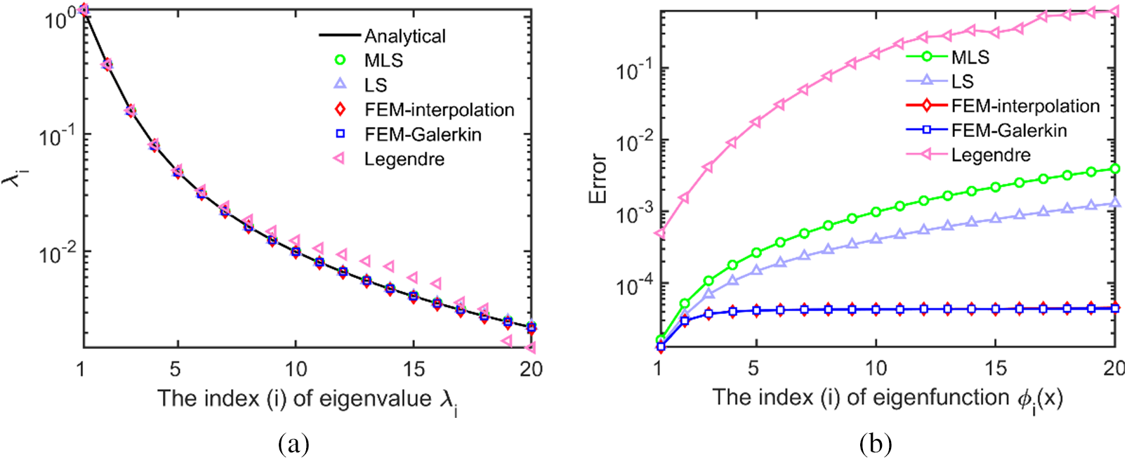
Figure 2: The eigenvalues (a) and the errors of eigenfunctions (b) of the exponential kernel function

Figs. 2a and 3a display the eigenvalues of examples 1 and 2, respectively, while Figs. 2b and 3b show the errors of eigenfunctions of examples 1 and 2, respectively. The computational formula is presented in Eq. (67). Fig. 3 indicates that the eigenvalues calculated using the interpolation method based on MLS, LS, and FEM are consistent with the analytical solutions. Additionally, the accuracy is close to that of the Galerkin method based on FEM, while the accuracy of the Galerkin method based on Legendre polynomials is slightly poor. Concerning the eigenfunctions, the accuracy of the FEM-based interpolation method is superior to or close to other methods, and it hardly fluctuates with an increase in the eigenfunction index. The accuracy of eigenfunctions calculated by the interpolation method based on MLS and LS is similar. In example 1, the error of eigenfunctions calculated using the Galerkin method based on the Legendre polynomial decreases rapidly as the eigenfunction index increases.

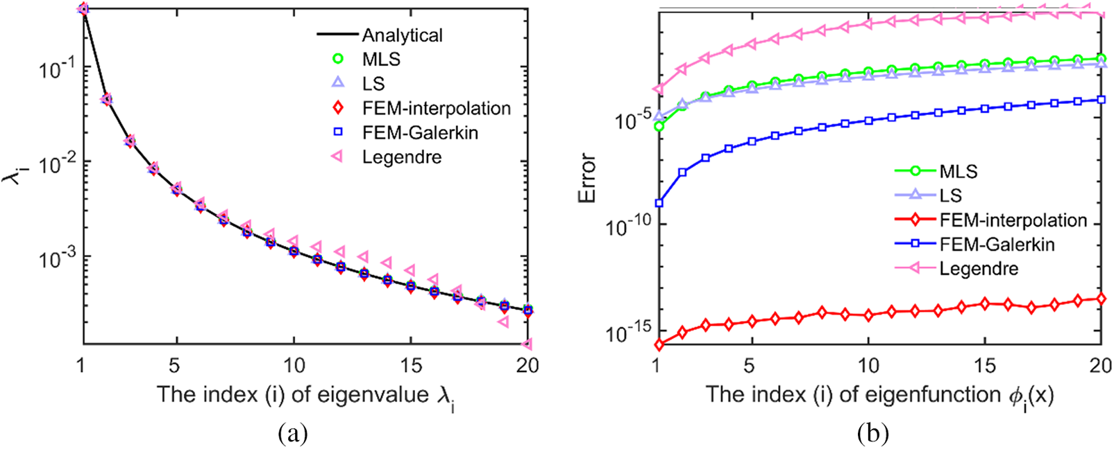
Figure 3: The eigenvalues (a) and the errors of eigenfunctions (b) of the Winer-Levy kernel function

To investigate the impact of various correlation lengths on eigenvalues, different correlation lengths (b=0.4,1,1.6, etc.) were selected for examples 1 and 3, and the results are presented in Fig. 4. The comparison of results presents that the correlation length has a more significant influence on the first few eigenvalues, and the longer the correlation length, the steeper the slope of the first few terms of the eigenvalue curve. The computed results of the MLS, LS, and FEM-interpolation are similar, indicating that the correlation length does not influence the accuracy of eigenvalues calculated using the interpolation method.

Figure 4: The eigenvalues of the exponential kernel function (a) and squared exponential kernel function (b) under different correlation lengths b

The preceding discussion confirms the accuracy of the methods. The subsequent discussion focuses on examining the impact of various parameters in the interpolation method on the computed results. For the FEM-based interpolation method, the relationship between the computed results and the number of nodes is investigated. Fig. 5 illustrates the mean of relative variance error ϵVar  (a) calculated from Eq. (62) and the mean of relative covariance error ϵCov (b) calculated from Eq. (63) for examples 1 and 2, respectively. The computed errors are compared with ϵVar  and ϵCov calculated from the analytical eigenvalues and eigenfunctions. The results demonstrate that ϵVar  and ϵCov calculated using the FEM-based interpolation method gradually converge as the number of nodes increases, when the number of nodes Nn is close to 120, the errors tend to converge, and ϵCov is less than ϵVar .

Figure 5: The mean of relative variance error ϵVar (a) and the mean of relative covariance error ϵCov (b) of examples 1 and 2 using the interpolation method based on FEM

In the case of MLS- and LS-based interpolation methods, this study mainly discusses the influence of the number of nodes Nn and the multiplier ds in the node support domain on the computed results. Figs. 6 and 7 show the mean of relative variance error ϵVar  (a) and the mean of relative covariance error ϵCov  (b) calculated using the MLS-based interpolation method in examples 1 and 2, respectively. The results indicate that as the number of nodes Nn increases, both ϵVar  and ϵCov gradually converge, and ϵCov is less than ϵVar . When the number of nodes is small, the multiplier ds has a significant influence on the error. However, as the number of nodes increases, the influence of the multiplier ds decreases rapidly, when the number of nodes Nn is close to 120, the influence of the multiplier ds tends to be small.

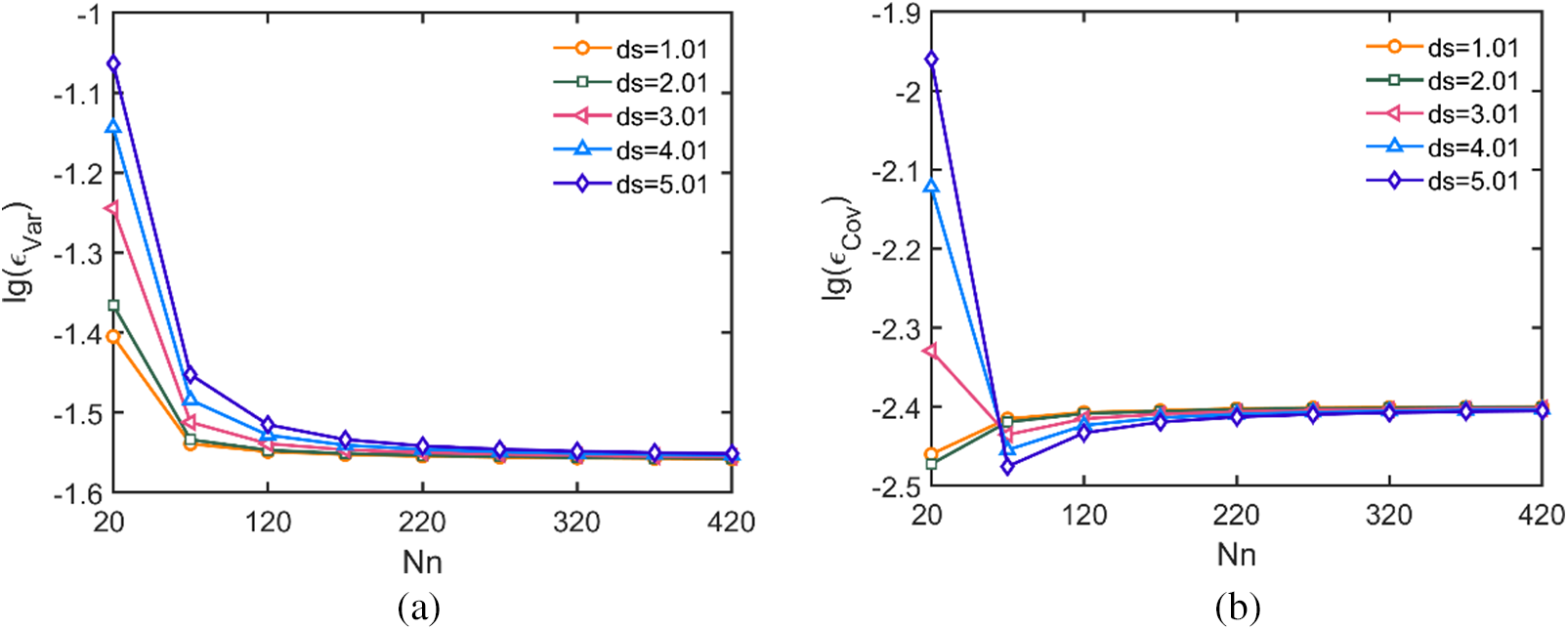
Figure 6: The convergence curves of the MLS-based interpolation method with respect to the number of nodes Nn in example 1, the mean of relative variance error ϵVar (a), the mean of relative covariance error ϵCov (b)

Figure 7: The convergence curves of the MLS-based interpolation method with respect to the number of nodes Nn in example 2, the mean of relative variance error ϵVar (a), the mean of relative covariance error ϵCov (b)

Fig. 8 displays the mean of the relative variance error ϵVar  (a) and the mean of the relative covariance error ϵCov  (b) calculated using the MLS-based interpolation method in example 3. In this example, the influence of the multiplier ds of the node support domain on the errors significantly increases. The smaller the multiplier ds, the lower the mean of relative variance error ϵVar (a) and the mean of relative covariance error ϵCov  (b), when the multiplier ds of the node support domain is closer to 1, the computational accuracy is higher. Under different ds, along with the increase of the number of nodes, ϵVar  and ϵCov  gradually decrease, the values of ϵVar  and ϵCov  in this example are two orders of magnitude smaller than those in examples 1 and 2, when Nn=120, ds=1.01, the values of ϵVar  and ϵCov  can reach 10−4.

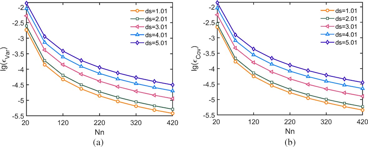
Figure 8: The convergence curves of the MLS-based interpolation method with respect to the number of nodes Nn in example 3, the mean of relative variance error ϵVar (a), the mean of relative covariance error ϵCov (b)

Figs. 9–11 display the mean of relative variance error ϵVar  (a) and the mean of relative covariance error ϵCov (b) calculated using the LS-based interpolation method in examples 1, 2 and 3, respectively. It is evident that when the multiplier ds of the node support domain is small, increasing the number of nodes does not enable the error to gradually converge. However, when the multiplier ds approaches 1, ϵVar  and ϵCov gradually converge with the increase of the number of nodes Nn except for the individual points of example 3. When Nn=120, ds=0.96, ϵVar  and ϵCov  tend to converge or obtained relatively good accuracy. Based on the comparison of the MLS- and LS-based interpolation methods, it is known that, in some examples, the MLS-based interpolation method is less sensitive to the multiplier ds of the node support domain, while the LS-based interpolation method is relatively sensitive and the multiplier ds should as close to 1 as possible. The reason is that, in the LS-based interpolation method, the more ds approaches 1, the more NI(xJ) approaches 1 when I=J. It is consistent with the requirement in the interpolation theory that NI(xJ) is equal to 1 when I=J and is equal to 0 when I≠J.

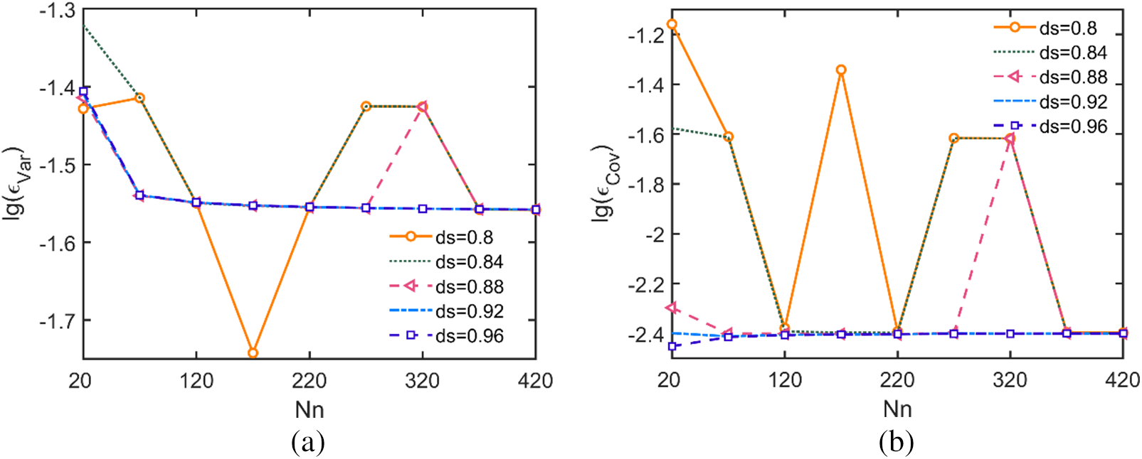
Figure 9: The convergence curves of the LS-based interpolation method with respect to the number of nodes Nn in example 1, the mean of relative variance error ϵVar (a), the mean of relative covariance error ϵCov (b)

Figure 10: The convergence curves of the LS-based interpolation method with respect to the number of nodes Nn in example 2, the mean of relative variance error ϵVar (a), the mean of relative covariance error ϵCov (b)

Figure 11: The convergence curves of the LS-based interpolation method with respect to the number of nodes Nn in example 3, the mean of relative variance error ϵVar  (a), the mean of relative covariance error ϵCov (b)

Table 1 displays other types of covariance functions with their corresponding parameters and domains. Meanwhile, the changes in the mean of the relative covariance error ϵCov concerning the number of truncating terms M are illustrated in Fig. 12. The results indicate that the MLS-, FEM-based interpolation method and the FEM-based Galerkin method yield similar outcomes regarding ϵCov, with the error decreasing as M increases. Conversely, the LS-based interpolation method produces comparable results to the previous three methods for covariance functions (b) and (d), but larger values for functions (a) and (c). Notably, the Legendre-based Galerkin method yields a higher value of ϵCov, which implies lower accuracy when compared to the other methods.

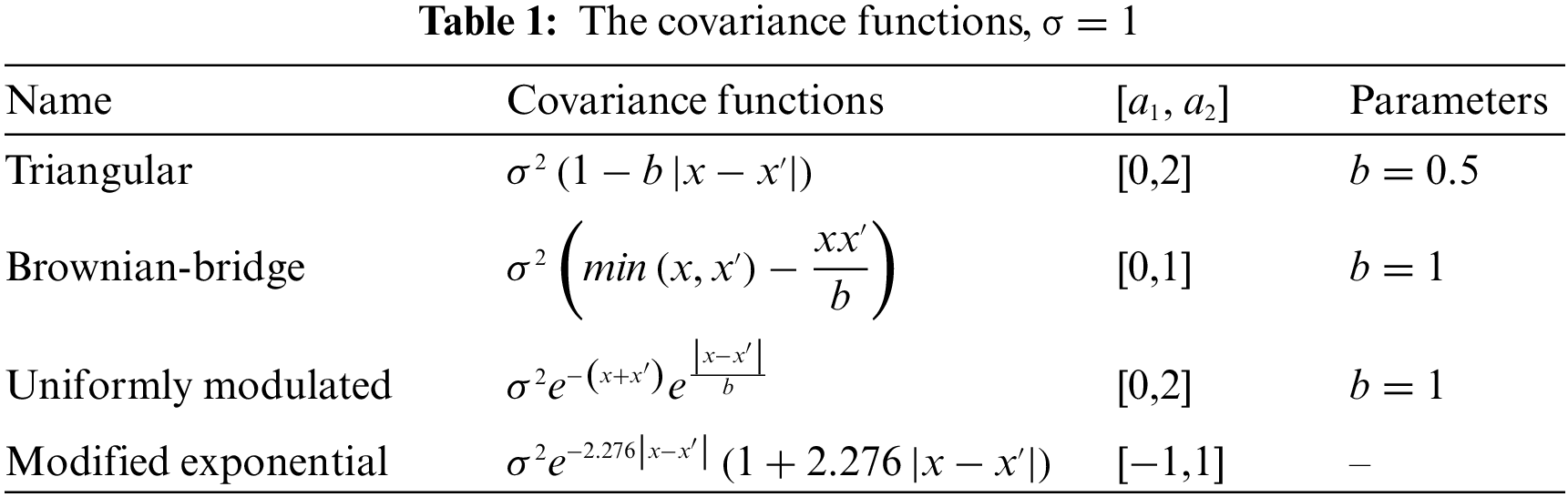
Figure 12: Variation of the mean of relative covariance error ϵCov with the number M of truncation. (a) Triangular, (b) brownian-bridge, (c) uniformly modulated, (d) modified exponential

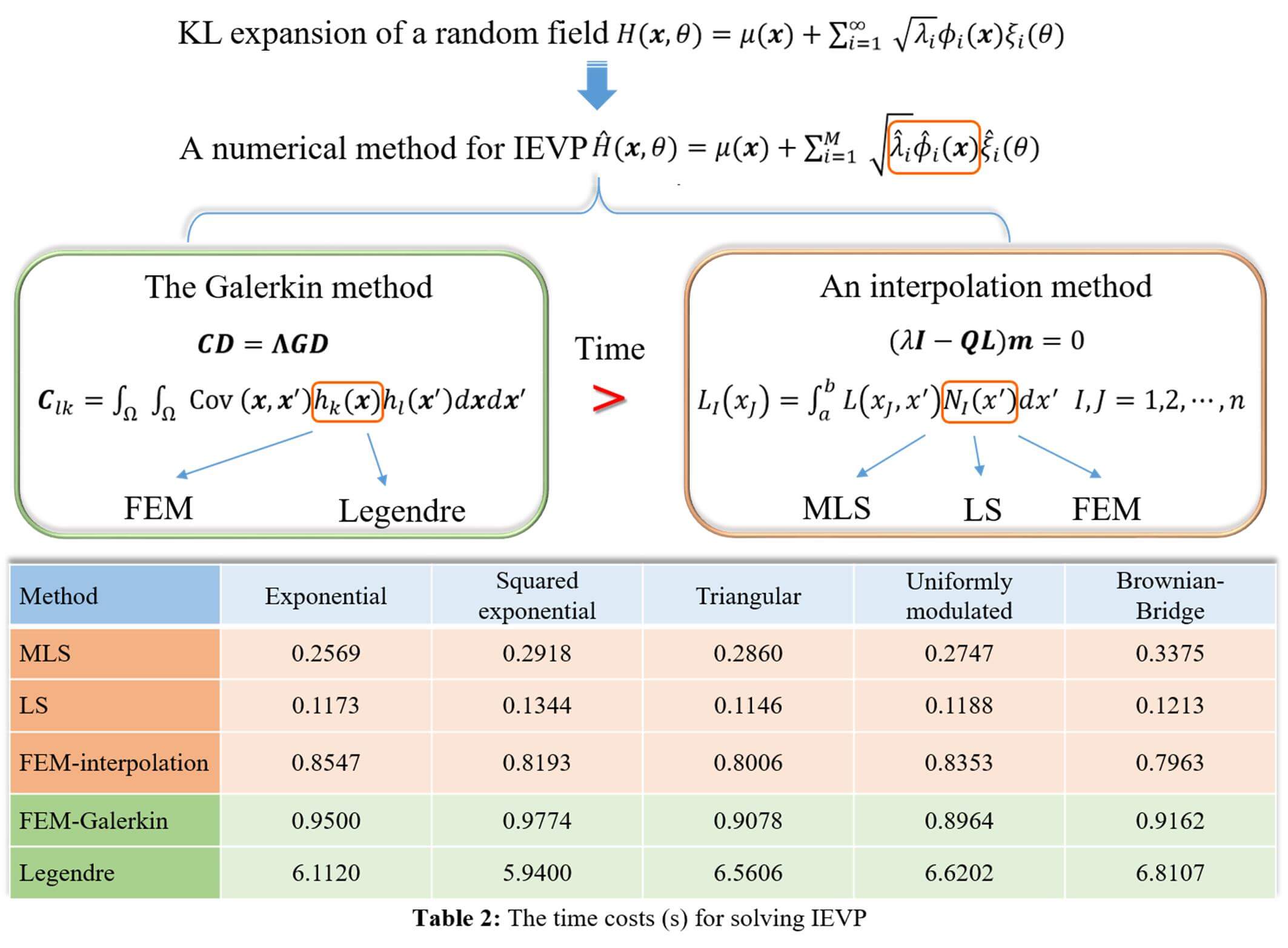
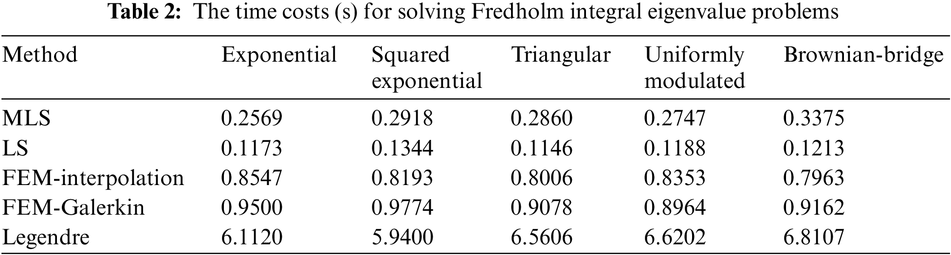
Table 2 presents a comparison of the computation times for solving Fredholm integral eigenvalue problems using various covariance functions. The methods employ the same number of nodes, while the number of truncating terms is fixed at M=20. The computations were performed on a computer equipped with an i7-4790 CPU @3.60 GHz. The findings demonstrate that the LS-based interpolation method is the most efficient, followed by the MLS- and FEM-based interpolation methods, with the FEM- and Legendre-based Galerkin method ranking last in terms of computational time. Notably, the Galerkin method utilizing Legendre polynomials requires an order of magnitude more time than the other methods. Hence, the interpolation method offers better computational efficiency than the Galerkin method. The reason for this is that in the process of solving eigenvalues and eigenfunctions, element Clk of matrix C in the Galerkin method as shown in Eq. (18) is a double integral, while element LI(xJ) of matrix L in the interpolation method as shown in Eq. (26) is a single integral.

4.3 Discretization of Two-Dimensional Random Fields and Stochastic Analysis

The following example is used to analyze the discretization of random fields in two-dimensional regular and irregular domains and is applied to stochastic analysis [37]. According to the one-dimensional analysis, we find that the interpolation method based on MLS and FEM can ensure both accuracy and relative stability. Therefore, in the following examples, we utilize MLS- and FEM-based interpolation methods for the discretization of random fields.

The provided Fig. 13 depicts a rectangular plate with a height of H=1.5m and a width of =1 m. The plate is fixed at the bottom and subjected to a uniform tensile stress of σ=1Pa along its upper edge. This is a plane stress problem, and Poisson’s ratio is ν=0.3. The modulus of elasticity E is supposed to be a random field with a mean value of μE=10Pa and a standard deviation of σE=2Pa. The covariance function is presented as follows:

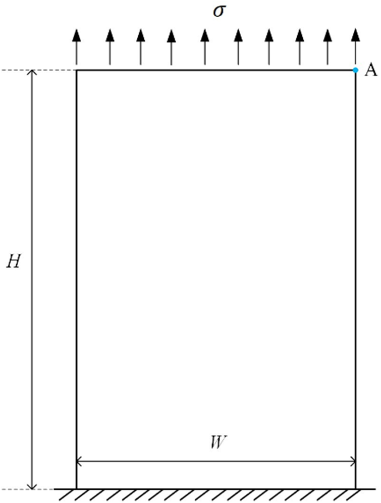
Figure 13: A rectangular plate

Cov(x,y)=σE2e−|x−x′|bxe−|y−y′|by(68)

The correlation length along the x direction is bx=0.5 m, while along the y direction, it is by=0.75 m. The covariance function takes on a two-dimensional form of the exponential kernel function, which exhibits analytical eigenvalues and eigenfunctions [37]. In KL expansion, the number of truncating terms is M=3. The Hermite polynomials are selected for the polynomial chaos expansion, and the order p=3. Fig. 14 displays the mesh used in the stochastic finite element method.

Figure 14: The mesh of the rectangular plate

Fig. 15 illustrates the probability density function of the vertical displacement UyA at point A on the plate. As seen that the probability density function calculated by the stochastic finite element method agrees well with the result by Monte Carlo (MC). Furthermore, the computed results based on the MLS and FEM techniques are found to closely match the analytical eigen-solutions, thus providing evidence for the validity of the MLS- and FEM-based interpolation methods for the KL expansion in two-dimensional domains.

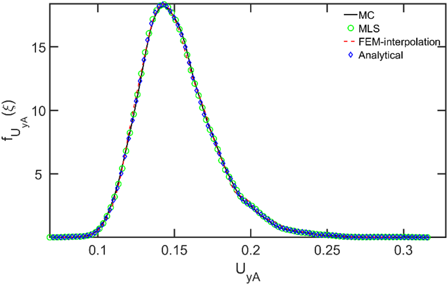
Figure 15: The probability density function fUyA(ξ) of the vertical displacement at point A

Fig. 16 presents the standard deviation σUy of the vertical displacement of the plate obtained using various methods. It is evident from (a), (b), and (c) that the variation trend of σUy derived through the MLS- and FEM-based interpolation techniques closely matches that of the analytical solution. Figs. 16d and 16e illustrate the absolute errors in displacement standard deviations for the MLS- and FEM-based interpolation methods relative to the analytical solution. The numerical outcomes reveal that both methods exhibit small absolute errors. However, the error associated with the MLS-based interpolation method is one order of magnitude lower than that of the FEM-interpolation method, indicating that the MLS-based interpolation approach is more accurate than the FEM-based interpolation method in this example.

Figure 16: The standard deviation σUy of vertical displacement of the plate: (a) MLS, (b) FEM-interpolation, (c) analytical, (d) absolute error of MLS and analytical, (e) absolute error of FEM-interpolation and analytical

To investigate the effect of the standard deviation of elastic modulus and polynomial chaos order on the standard deviation of the vertical displacement of a plate, observation point A was selected. Fig. 17 depicts the standard deviation σUyA of the vertical displacement of point A for polynomial chaos order p=1,2, and 3 as (a), (b), and (c), respectively. The results demonstrate that as the standard deviation σE of elastic modulus E increases, σUyA gradually increases, with negligible differences among the results obtained using MLS-, FEM-based interpolation, and analytical eigen-solutions. Furthermore, as the standard deviation of the input random parameters increases, higher polynomial orders are required to achieve better accuracy.

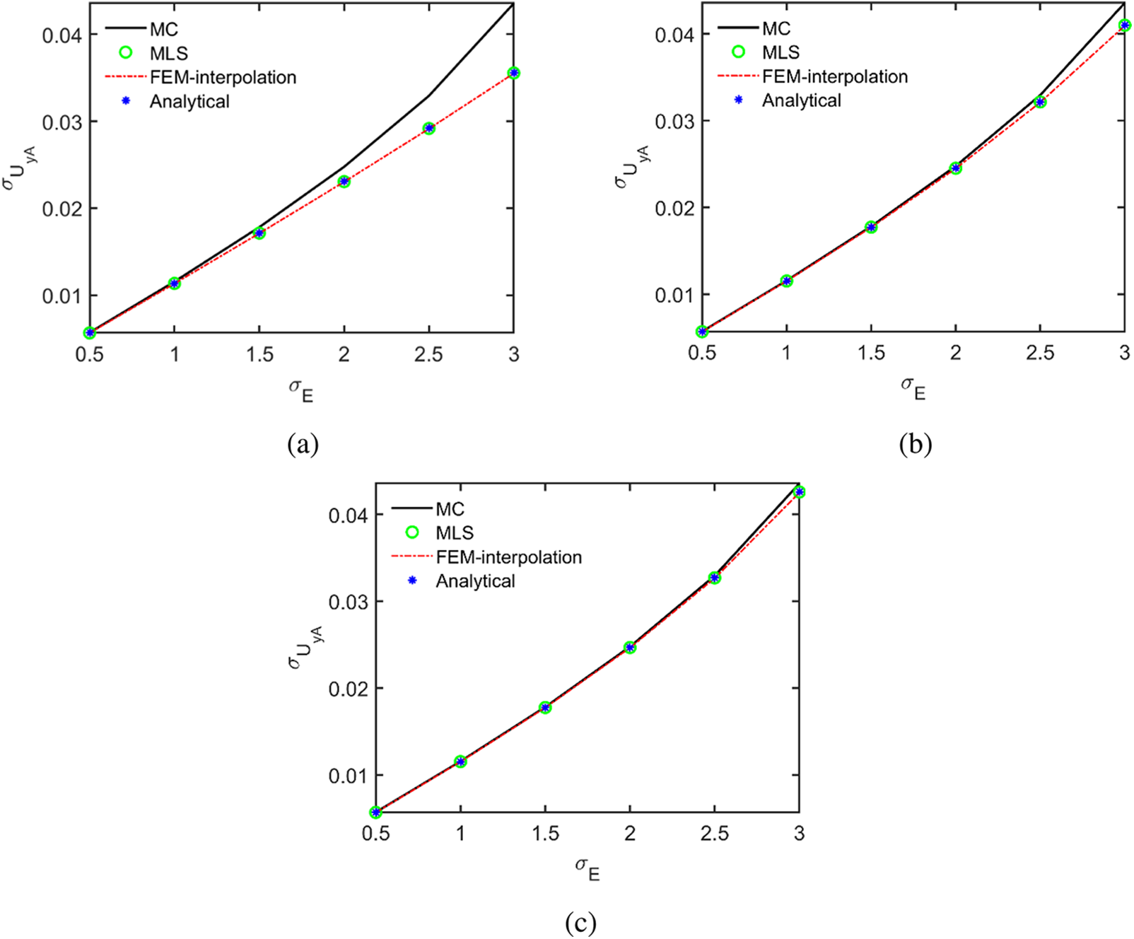
Figure 17: The standard deviation σUyA of vertical displacement of point A varies with the standard deviation σE of the elastic modulus E, (a) the order of polynomial chaos p=1, (b) the order of polynomial chaos p=2 (c) the order of polynomial chaos p=3

To compare the applicability of different methods for the discretization of random fields in two-dimensional irregular domains, a square plate with a pentagonal hole, as shown in Fig. 18, was calculated and subjected to random analysis. The length of the plate is L=2m, the left edge of the plate is fixed, while a uniformly distributed load σ=1 Pa is applied to the other edge. The central coordinate of the hole is equal to xc=1,yc=1, the radius is R=0.3+0.08×sin⁡(5α), where α∈[0,2π] rotates counterclockwise from the horizontal direction. The model is a plane stress problem, with Poisson’s ratio ν=0.3. It is assumed that the elastic modulus E is a Gaussian random field, with a mean μE=20Pa, and a standard deviation σE=5Pa. The covariance function of the random field is the same as that of the previous example, and the correlation lengths are bx=1 m and by=1 m.

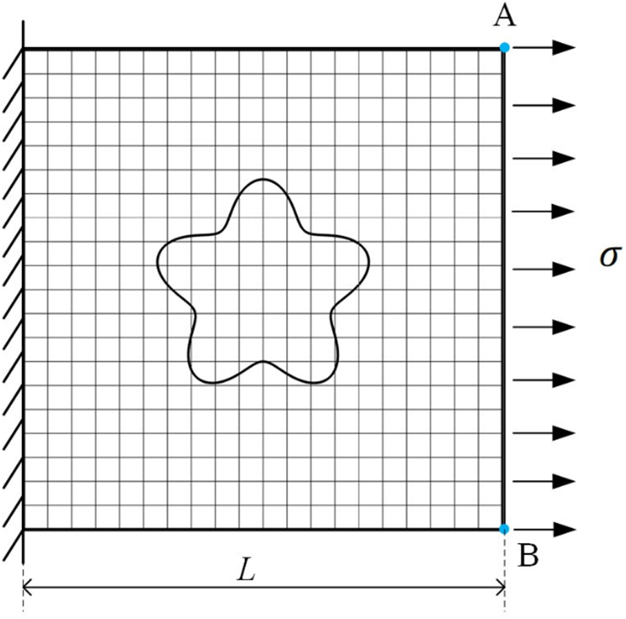
Figure 18: A square plate and the XFEM mesh

As the plate with a hole has an irregular domain, the basis function in the extended finite element method can be used to replace the finite element basis function when IEVP is solved in the discretization of random fields. The level set function is used to determine whether the node is in the plate. If the elements are cut by hole edge, only the part of the elements in the plate is integrated. The method is expressed as XFEM-interpolation. Meanwhile, in the subsequent stochastic analysis, the extended finite element method is combined with PCE, and the number of truncating terms is M=3, the order of polynomial chaos is p=3.

An illustration of the different distribution modes of the MLS-based interpolation method used to solve the IEVP is presented in Fig. 19. Specifically, Fig. 19a shows a uniform distribution without considering the internal hole boundary, while Fig. 19b shows a scattering distribution that takes into account the internal hole boundary. A comparison between the uniform and scattering distributions are conducted by the eigenvalues which are presented in Table 3. the results show that the errors of the two distribution mode are approximately 10−4. These findings suggest that different distribution modes have little impact on the accuracy of the discretization of random fields, and for convenience, the distribution mode shown in Fig. 19a is selected for subsequent computations.

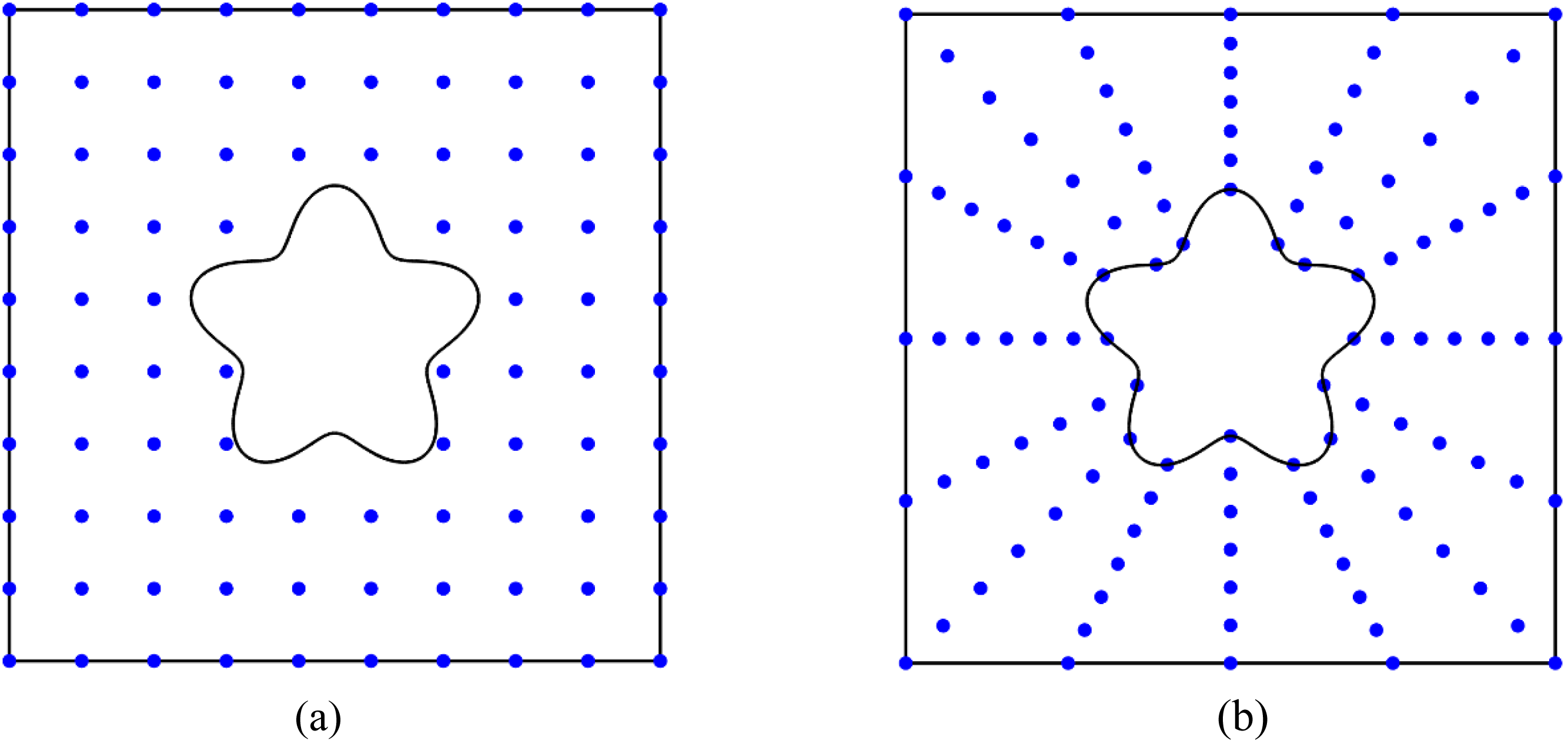
Figure 19: The distributions of points of MLS-based interpolation method, (a) uniform distribution, (b) scattering distribution

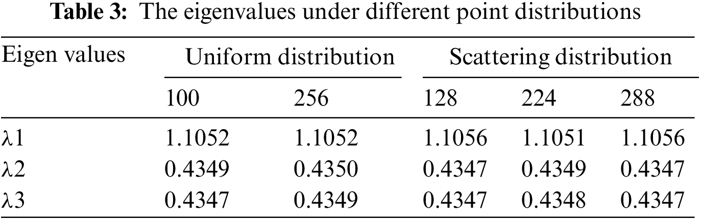
Table 4 displays the standard deviations σUxA and σUxB of the horizontal displacement at point A and point B, respectively, which were obtained by the MLS-based interpolation method under various correlation lengths. The table demonstrates that both σUxA and σUxB gradually increase with increasing correlation lengths in both the x and y directions. Moreover, if one correlation length is fixed and the other increases, both σUxA and σUxB also gradually increase. Additionally, the impact of the correlation length in the x direction on the standard deviation of the horizontal displacement is significantly greater than that of the y direction.

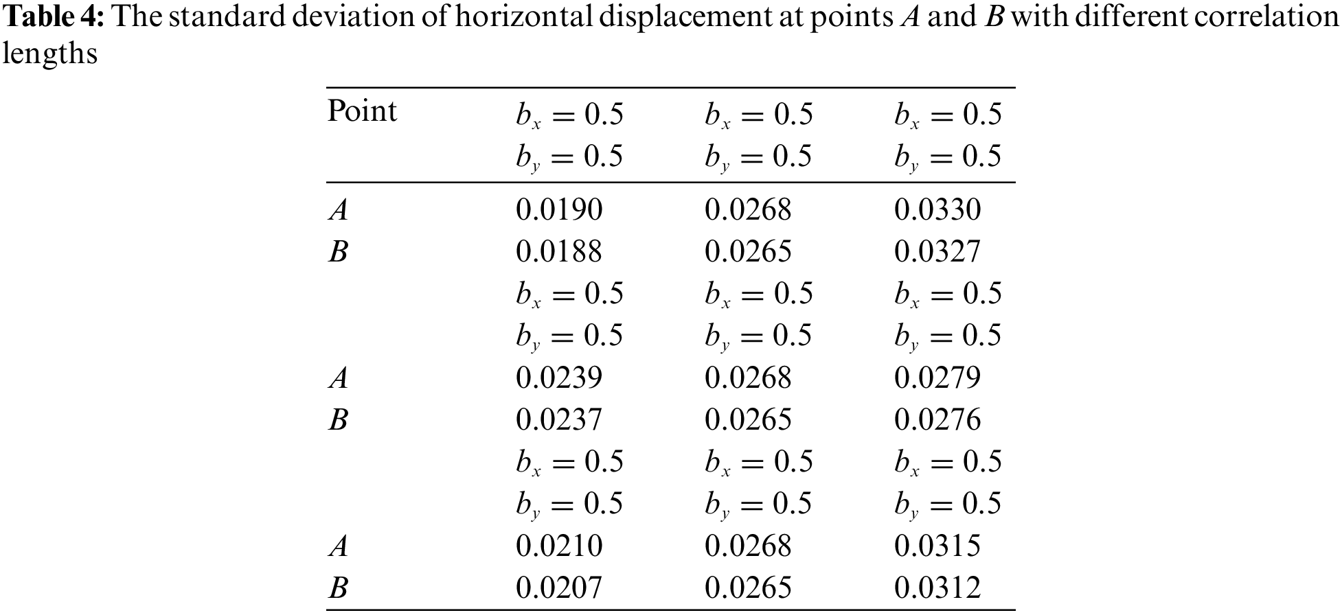
Fig. 20 illustrates the distribution of the standard deviation of horizontal displacement σUx of the plate obtained using MLS-based interpolation method (a) and XFEM-based interpolation method (b). The discretization of random fields used 10×10 nodes based on MLS and 21×21 mesh nodes based on XFEM basis functions, while the stochastic analysis employed a mesh node of 21×21 for XFEM. The figure shows that the two methods produced similar trends in the distribution of σUx, with the maximum value located at the middle of the right end of the plate. This suggests that the basis functions of XFEM can serve as interpolation basis functions for computing in complex domains.

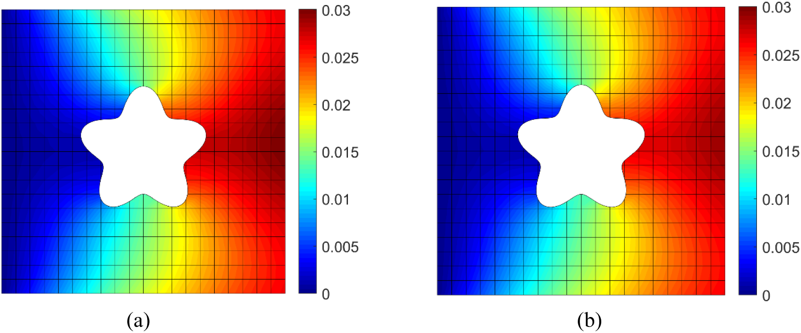
Figure 20: The standard deviation of horizontal displacement σUx: (a) MLS, (b) XFEM-interpolation

The XFEM calculations presented in the previous discussion employed the same mesh for both the discretization of the random field and stochastic analysis. However, the XFEM permits different meshes for the two processes. Nevertheless, applying eigenfunctions during stochastic analysis involves multiple transformations between global and local coordinates. In contrast, the MLS-based interpolation method enables the separation of distribution points and meshes in random field discretization and stochastic analysis without requiring any coordinate transformation. Hence, when a large number of meshes are used for stochastic analysis, the MLS-based interpolation method by point interpolation without meshing confers more advantages.

5  Conclusions

This study proposes an interpolation method for solving Fredholm integral eigenvalue problems in KL expansion for random field discretization. The performance of three interpolation basis functions, namely MLS, LS, and FEM, is evaluated. Compared to the Galerkin method, which uses finite element or Legendre polynomials as basis functions and involves a two-folded integral to calculate the integral matrix containing the covariance function, the proposed interpolation method only requires a single integral, resulting in reduced computational time. Numerical examples in one-dimensional domains reveal the validity and computational efficiency of the proposed method. The LS-based interpolation method is the most efficient, and the closer the multiplier of the node support domain is to 1, the higher the accuracy is. While the MLS-based interpolation method produces more stable results than LS, and the influence of the multiplier decreases with a large number of nodes. The FEM-based interpolation method has high accuracy, and the accuracy of the eigenfunction is almost independent of the eigenfunction index.

Additionally, this study combines KL expansion and PCE to perform random analysis in two-dimensional regular and irregular domains. The results show that MLS-based interpolation provides higher computational accuracy than FEM-based interpolation in two-dimensional regular domains. As the standard deviations of the input random parameters increase, higher orders of polynomials are needed to achieve better results. In two-dimensional irregular domains, XFEM is used for stochastic analysis. The XFEM basis function can serve as the interpolation basis function, and MLS-based interpolation can be performed using uniformly distributed points for random field discretization.

Acknowledgement: The authors are grateful for the support by the Postgraduate Research & Practice Program of Jiangsu Province (Grant No. KYCX18_0526), the Fundamental Research Funds for the Central Universities (Grant No. 2018B682X14) and Guangdong Basic and Applied Basic Research Foundation (No. 2021A1515110807).

Funding Statement: The authors gratefully acknowledge the support provided by the Postgraduate Research & Practice Program of Jiangsu Province (Grant No. KYCX18_0526), the Fundamental Research Funds for the Central Universities (Grant No. 2018B682X14) and Guangdong Basic and Applied Basic Research Foundation (No. 2021A1515110807).

Author Contributions: The authors confirm contribution to the paper as follows: study conception and design: Zi Han; data collection: Zi Han; analysis and interpretation of results: Zi Han; draft manuscript preparation: Zi Han, Zhentian Huang. All authors reviewed the results and approved the final version of the manuscript.

Availability of Data and Materials: The data undering this article will be shared on reasonable request to the corresponding author.

Conflicts of Interest: The authors declare that they have no conflicts of interest to report regarding the present study.

References

1. Allaix, D. L., Carbone, V. I. (2009). Discretization of 2D random fields: A genetic algorithm approach. Engineering Structures, 31(5), 1111–1119. https://doi.org/10.1016/j.engstruct.2009.01.008 [Google Scholar] [CrossRef]

2. Betz, W., Papaioannou, I., Straub, D. (2014). Numerical methods for the discretization of random fields by means of the Karhunen–Loève expansion. Computer Methods in Applied Mechanics and Engineering, 271(5), 109–129. https://doi.org/10.1016/j.cma.2013.12.010 [Google Scholar] [CrossRef]

3. Der Kiureghian, A., Ke, J. B. (1988). The stochastic finite element method in structural reliability. Probabilistic Engineering Mechanics, 3(2), 83–91. https://doi.org/10.1016/0266-8920(88)90019-7 [Google Scholar] [CrossRef]

4. Vanmarcke, E. (2010). Random fields: Analysis and synthesis. 2nd edition. Singapore: World Scientific Publishing. [Google Scholar]

5. Liu, W. K., Belytschko, T., Mani, A. (1986). Random field finite elements. International Journal for Numerical Methods in Engineering, 23(10), 1831–1845. https://doi.org/10.1002/(ISSN)1097-0207 [Google Scholar] [CrossRef]

6. Li C. C, Der Kiureghian A. (1993). Optimal discretization of random fields. Journal of Engineering Mechanics, 119(6), 1136–1154. https://doi.org/10.1061/(ASCE)0733-9399(1993)119:6(1136) [Google Scholar] [CrossRef]

7. Zhang, X., Liu, Q., Huang, H. (2019). Numerical simulation of random fields with a high-order polynomial based Ritz–Galerkin approach. Probabilistic Engineering Mechanics, 55(9), 17–27. https://doi.org/10.1016/j.probengmech.2018.08.003 [Google Scholar] [CrossRef]

8. Dai, H. Z., Zhang, R. J., Beer, M. (2022). A new perspective on the simulation of cross-correlated random fields. Structural Safety, 96(2), 102201. https://doi.org/10.1016/j.strusafe.2022.102201 [Google Scholar] [CrossRef]

9. Zhang, J., Ellingwood, B. (1994). Orthogonal series expansions of random fields in reliability analysis. Journal of Engineering Mechanics, 120(12), 2660–2677. https://doi.org/10.1061/(ASCE)0733-9399(1994)120:12(2660) [Google Scholar] [CrossRef]

10. Ghanem, R. G., Spanos, P. D. (1991). Stochastic finite elements: A spectral approach. New York: Springer. [Google Scholar]

11. Aldosary, M., Wang, J., Li, C. (2018). Structural reliability and stochastic finite element methods: State-of-the-art review and evidence-based comparison. Engineering Computations, 35(6), 2165–2214. https://doi.org/10.1108/EC-04-2018-0157 [Google Scholar] [CrossRef]

12. Huang, S., Quek, S., Phoon, K. (2001). Convergence study of the truncated Karhunen–Loeve expansion for simulation of stochastic processes. International Journal for Numerical Methods in Engineering, 52(9), 1029–1043. https://doi.org/10.1002/nme.255 [Google Scholar] [CrossRef]

13. Papaioannou, I. (2012). Non-intrusive finite element reliability analysis methods (Ph.D. Thesis). Technical University Munich, Germany. [Google Scholar]

14. Liu, Q., Zhang, X. (2017). A Chebyshev polynomial-based Galerkin method for the discretization of spatially varying random properties. Acta Mechanica, 228(6), 2063–2081. https://doi.org/10.1007/s00707-017-1819-2 [Google Scholar] [CrossRef]

15. Stefanou, G., Papadrakakis, M. (2007). Assessment of spectral representation and Karhunen–Loève expansion methods for the simulation of Gaussian stochastic fields. Computer Methods in Applied Mechanics and Engineering, 196(21–24), 2465–2477. https://doi.org/10.1016/j.cma.2007.01.009 [Google Scholar] [CrossRef]

16. Schwab, C., Todor, R. A. (2006). Karhunen–Loève approximation of random fields by generalized fast multipole methods. Journal of Computational Physics, 217(1), 100–122. https://doi.org/10.1016/j.jcp.2006.01.048 [Google Scholar] [CrossRef]

17. Basmaji, A., Dannert, M., Nackenhorst, U. (2022). Implementation of Karhunen–Loève expansion using discontinuous Legendre polynomial based Galerkin approach. Probabilistic Engineering Mechanics, 67(2), 103176. https://doi.org/10.1016/j.probengmech.2021.103176 [Google Scholar] [CrossRef]

18. Rahman, S., Xu, H. (2005). A meshless method for computational stochastic mechanics. International Journal for Computational Methods in Engineering Science and Mechanics, 6(1), 41–58. https://doi.org/10.1080/15502280590888649 [Google Scholar] [CrossRef]

19. Rahman, S. (2018). A Galerkin isogeometric method for Karhunen–Loève approximation of random fields. Computer Methods in Applied Mechanics and Engineering, 338, 533–561. https://doi.org/10.1016/j.cma.2018.04.026 [Google Scholar] [CrossRef]

20. Belytschko, T., Lu, Y. Y., Gu, L. (1994). Element-free Galerkin methods. International Journal for Numerical Methods in Engineering, 37(2), 229–256. https://doi.org/10.1002/(ISSN)1097-0207 [Google Scholar] [CrossRef]

21. Huang, Z., Lei, D., Han, Z., Zhang, P. (2019). Boundary moving least square method for numerical evaluation of two-dimensional elastic membrane and plate dynamics problems. Engineering Analysis with Boundary Elements, 108(4), 41–48. https://doi.org/10.1016/j.enganabound.2019.08.002 [Google Scholar] [CrossRef]

22. Liu, W. K., Li, S., Belytschko, T. (1997). Moving least-square reproducing kernel methods (I) methodology and convergence. Computer Methods in Applied Mechanics and Engineering, 143(1–2), 113–154. https://doi.org/10.1016/S0045-7825(96)01132-2 [Google Scholar] [CrossRef]

23. Nayroles, B., Touzot, G., Villon, P. (1992). Generalizing the finite element method: Diffuse approximation and diffuse elements. Computational Mechanics, 10(5), 307–318. https://doi.org/10.1007/BF00364252 [Google Scholar] [CrossRef]

24. Li, S., Liu, W. K. (1999). Reproducing kernel hierarchical partition of unity, Part I– formulation and theory. International Journal for Numerical Methods in Engineering, 45, 251–288. [Google Scholar]

Li, S., Lu, H., Han, W., Liu, W. K., Simkins, D. C. (2004). Reproducing kernel element method Part II: Globally conforming Im/Cn hierarchies. Computer Methods in Applied Mechanics and Engineering, 193, 953–987. [Google Scholar]

26. Yu, H., Li, S. (2021). On approximation theory of nonlocal differential operators. International Journal for Numerical Methods in Engineering, 122, 6984–7012. [Google Scholar]

27. Moës, N., Dolbow, J., Belytschko, T. (1999). A finite element method for crack growth without remeshing. International Journal for Numerical Methods in Engineering, 46(1), 131–150. [Google Scholar]

28. Belytschko, T., Black, T. (1999). Elastic crack growth in finite elements with minimal remeshing. International Journal for Numerical Methods in Engineering, 45(5), 601–620. [Google Scholar]

29. Melenk, J. M., Babuška, I. (1996). The partition of unity finite element method: Basic theory and applications. Computer Methods in Applied Mechanics and Engineering, 139(14), 289–314. https://doi.org/10.1016/S0045-7825(96)01087-0 [Google Scholar] [CrossRef]

30. Sukumar, N., Chopp, D. L., Moës, N., Belytschko, T. (2001). Modeling holes and inclusions by level sets in the extended finite-element method. Computer Methods in Applied Mechanics and Engineering, 190(46–47), 6183–6200. https://doi.org/10.1016/S0045-7825(01)00215-8 [Google Scholar] [CrossRef]

31. Trees, H. L. V. (1968). Detection, estimation and modulation theory. New York: Wiley. [Google Scholar]

32. Phoon, K. K., Huang, S. P., Quek, S. T. (2002). Simulation of second-order processes using Karhunen–Loeve expansion. Computers and Structures, 80(12), 1049–1060. https://doi.org/10.1016/S0045-7949(02)00064-0 [Google Scholar] [CrossRef]

33. Sakamoto, S., Ghanem, R. (2002). Polynomial chaos decomposition for the simulation of non-Gaussian nonstationary stochastic processes. Journal of Engineering Mechanics, 128(2), 190–201. https://doi.org/10.1061/(ASCE)0733-9399(2002)128:2(190) [Google Scholar] [CrossRef]

34. Dai, H. Z., Zheng, Z. B., Ma, H. H. (2019). An explicit method for simulating non-Gaussian and non-stationary stochastic processes by Karhunen–Loève and polynomial chaos expansion. Mechanical Systems and Signal Processing, 115(4), 1–13. https://doi.org/10.1016/j.ymssp.2018.05.026 [Google Scholar] [CrossRef]

35. Tong, M. N., Zhao, Y. G., Zhao, Z. (2021). Simulating strongly non-Gaussian and non-stationary processes using Karhunen–Loève expansion and L-moments-based Hermite polynomial model. Mechanical Systems and Signal Processing, 160(2), 107953. https://doi.org/10.1016/j.ymssp.2021.107953 [Google Scholar] [CrossRef]

36. Zhang, X. D., Bui, T. Q. (2015). A fictitious crack XFEM with two new solution algorithms for cohesive crack growth modeling in concrete structures. Engineering Computations, 32(2), 473–497. https://doi.org/10.1108/EC-08-2013-0203 [Google Scholar] [CrossRef]

37. Ghanem, R. G., Spanos, P. D. (2003). Stochastic finite elements: A spectral approach. New York: Springer. [Google Scholar]