
 Submit a Paper
 Propose a Special lssue
 Open Access
ARTICLE

Fractal Fractional Order Operators in Computational Techniques for Mathematical Models in Epidemiology
1 Institue of Mathematics, Khwaja Fareed University of Enginnering and Information Technology, Raheem Yar Khan, Pakistan
2 Department of Computer Science and Mathematics, Lebanese American University, Beirut, Lebanon
3 Department of Mathematics, Art and Science Faculty, Siirt University, Siirt, 56100, Turkey
4 Department of Mathematics, Mathematics Research Center, Near East University, Nicosia, Turkey
5 Department of Computer Engineering, Biruni University, Istanbul, 34010, Turkey
6 Department of Hospitality Services, Babes-Bolyai University, Cluj-Napoca, 400174, Romania
7 Department of Pharmaceutical Sciences, Vasile Goldiș Western University of Arad, Arad, 310025, Romania
8 Department of Mathematics and Informatics, Faculty of Sciences, Lucian Blaga University of Sibiu, Sibiu, 550012, Romania
9 Department of Electronics and Communication Engineering, Saveetha School of Engineering, SIMATS, Chennai, Tamilnadu, India
* Corresponding Authors: Ali Akgül. Email: ; Amelia Bucur. Email:
(This article belongs to the Special Issue: Recent Developments on Computational Biology-I)
Computer Modeling in Engineering & Sciences 2024, 138(2), 1385-1403. https://doi.org/10.32604/cmes.2023.028803
Received 08 January 2023; Accepted 09 June 2023; Issue published 17 November 2023
 View Full Text
 Download PDF
Abstract
New fractional operators, the COVID-19 model has been studied in this paper. By using different numerical techniques and the time fractional parameters, the mechanical characteristics of the fractional order model are identified. The uniqueness and existence have been established. The model’s Ulam-Hyers stability analysis has been found. In order to justify the theoretical results, numerical simulations are carried out for the presented method in the range of fractional order to show the implications of fractional and fractal orders. We applied very effective numerical techniques to obtain the solutions of the model and simulations. Also, we present conditions of existence for a solution to the proposed epidemic model and to calculate the reproduction number in certain state conditions of the analyzed dynamic system. COVID-19 fractional order model for the case of Wuhan, China, is offered for analysis with simulations in order to determine the possible efficacy of Coronavirus disease transmission in the Community. For this reason, we employed the COVID-19 fractal fractional derivative model in the example of Wuhan, China, with the given beginning conditions. In conclusion, again the mathematical models with fractional operators can facilitate the improvement of decision-making for measures to be taken in the management of an epidemic situation.Keywords
Coronavirus (COVID-19) is a new phenomenon in recent days, which affected the entire world while it was emerging. According to reference [1], it is reported that a mysterious outbreak of atypical pneumonia was traced to a seafood market in Wuhan, China. In December 2019 the first case of novel coronavirus was reported. The symptoms of coronavirus are dry cough, fever, fatigue and in severe cases, acute respiratory syndrome that appears in 2–10 days which further causes pneumonia, kidney failure and even death [2]. In between March and April, coronavirus became a global phenomenon with the whole world facing an emergency situation. Initial cases were reported in the wet seafood market of Wuhan, China [3]. That is why some researchers thought that it is transmitted by animals to humans. This virus is transmitted from one person to another through physical contact, droplets during sneezing and coughing [4]. Researchers in the field of epidemiology and other fields of biology are trying hard to develop the cure based on ongoing clinical trials, but different researching companies from different countries have developed the vaccine for COVID-19 in [5]. Developed countries like the USA, UK, Italy, Spain and many others are affected very badly, most of the global deaths are being reported from these countries [6]. Mathematical modeling is used to understand the dynamics and behavior of disease and then develop the procedures for the treatment of disease. For this purpose, many researchers developed the COVID-19 models (see [7–12]). Reproductive number has a notable role in the analysis of mathematical models. Reproductive number explains the behavior of the simulation of COVID-19. The fractional order mathematical models of a few more infectious diseases have recently been studied in [13].
In order to address problems in the real world, fractional calculus (FC) is essential. It is widely utilized in a variety of scientific, engineering, and financial sectors. The key characteristics of FC are fractional integrals and derivatives of fractional order. Researchers’ interest in fractional calculus and the numerous aspects of that study under inquiry has grown in recent years. This is due to the fact that genetic mutations are a crucial tool for characterizing the dynamic operation of diverse biological systems. These component operators’ non-local properties, which are absent from the integer separator operator, give them their power [14–16]. For the development of an artificial pancreas, Farman et al. [17] employed an Atangana Baleanu derivative to manage glucose levels in insulin treatments. Differential equations with various generalized fractional derivatives have been solved using a variety of numerical techniques [18–20]. In [21], a generalization of the squared remainder minimization method for resolving multi-term fractional differential equations was developed. The Caputo time-fractional derivative and redefined extended B-spline functions have been used for the time and spatial discretization, respectively in [22–25] and some details are also given in [26–28]. COVID-19 outbreaks have been well modeled in [29–31] for a variety of geographic locations. Additionally, some publications [32–34] explored the impact of quarantine and social isolation on the viral load in the environment. For the COVID-19 epidemic, some researchers suggested the best control approaches including cost-effectiveness assessments [35,36].
2 Basic Concepts of Fractional Operators
In this section, we consider some definition related to fractal fractional operator given in [31,34,37,38].
Definition 2.1: Let
Definition 2.2: Let
where
Definition 2.3: Let
where
Definition 2.4: The function
Definition 2.5: The function
Definition 2.6: The function
3 Fractal Fractional Order Model
We suppose the COVID-19 model formulated by Ahmad et al. [39]. In this model,
with initial conditions are
In this section, we will discuss the equilibrium points of the given COVID-19 model (7). Equilibrium points have two types namely as disease free equilibrium and endemic equilibrium. We obtained these points by putting the number zero on the right side of the system (7). We suppose that E’ represents disease free equilibrium and endemic equilibrium is represented by E*. If we take both of our equilibriums, we have
We obtain the basic reproductive number
4 Existence and Stability Theory
We consider [40]
where
We can write system (9) as:
By replacing
where
We describe a Banach space
Define as operator
We suppose that
• For each
• Considering
Theorem 4.1: Suppose that the state (11) exists. Let
Proof: First of all, considering the Eq. (10) is completely continuous which is described by operator
Suppose that
Therefore, we get
When
Thus,
Theorem 4.2: [38] Suppose that the condition (12) holds. If
Then the solution of the system is unique.
Proof: For all
Therefore,
We denote by:
Let
Theorem 4.3: [44] Let
(i) A is a matrix which converges to zero;
(ii)
(iii) The modulus for every eigen-values of A is lower than 1;
(iv) The matrix I—A is non-singular, with
We give the following theorem, for the hypothesis that
Theorem 4.4: Let
then, the semi linear inclusion system:
has at least one solution in
Proof: The theorem is a particular case of Theorem 3.11 from [44]. It is demonstrated the same as Theorem 3.11 from [44], with
The demonstration of the theorem uses elements from the fixed-point theory and results from the fact that
Definition 4.1: The system is Ulam-Hyers stable if
And there exists unique solution
•
•
Lemma 4.1: Perturbed solution for the system according the given result in [37].
satisfies the following relation:
We note:
Lemma 4.2: The solution of the system is Ulam-Hyers stable if
Proof: Suppose that
Consequently, one can write
We can write the above relation is
where
4.3 Fractal-Fractional Integral with Mittag-Leffler Kernel
Consider:
We construct the numerical scheme at
Applying the approximation of the integrals on the right hand side of system (18) yields:
We consider
Then, we have
5 Computational Result and Discussion
COVID-19 fractional order model for the case of Wuhan, China, is offered for analysis with simulations in order to determine the possible efficacy of Coronavirus disease transmission in the Community. For this reason, we employed the COVID-19 fractal fractional derivative model in the example of Wuhan, China, with the given beginning conditions. The parameters of actual data are described in detail in [46]. By using different numerical techniques and the time fractional parameters, the mechanical characteristics of the fractional order model are identified. The findings of fractional value calculations were used to detect the outcomes of the nonlinear system memory. It provides a better way than wanting to control the disease without defining other parameters.
In Figs. 1–4, simulations were obtained by fractal fractional method. It is noted that physical procedures are far better explained using the fractional order derivatives which are the most notable and sustainable component compared to the classical-order case with order at 1. The behaviors of the dynamics found in the various fractional orders are shown in the form of numerical results that have been reported.
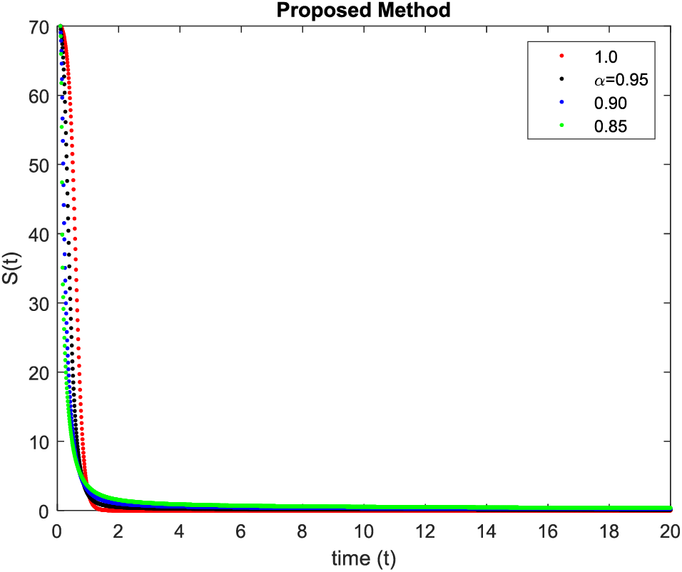
Figure 1: Simulation of
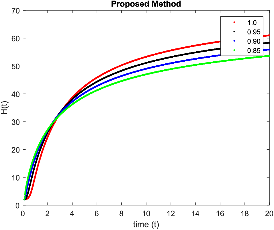
Figure 2: Simulation of
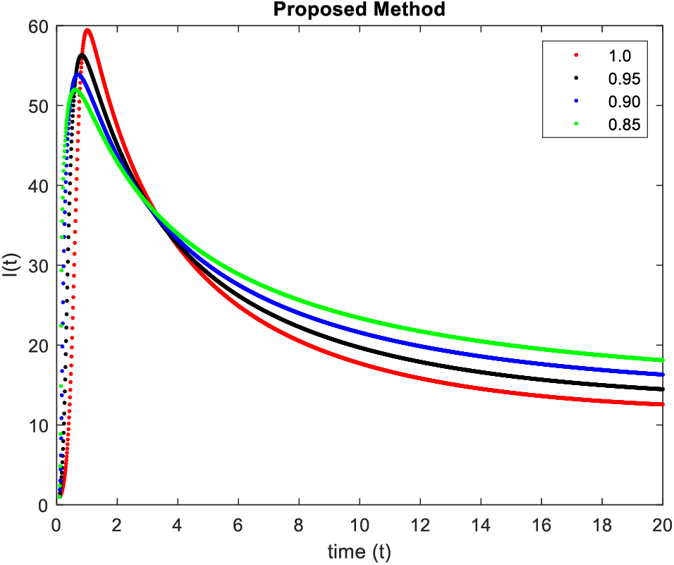
Figure 3: Results of
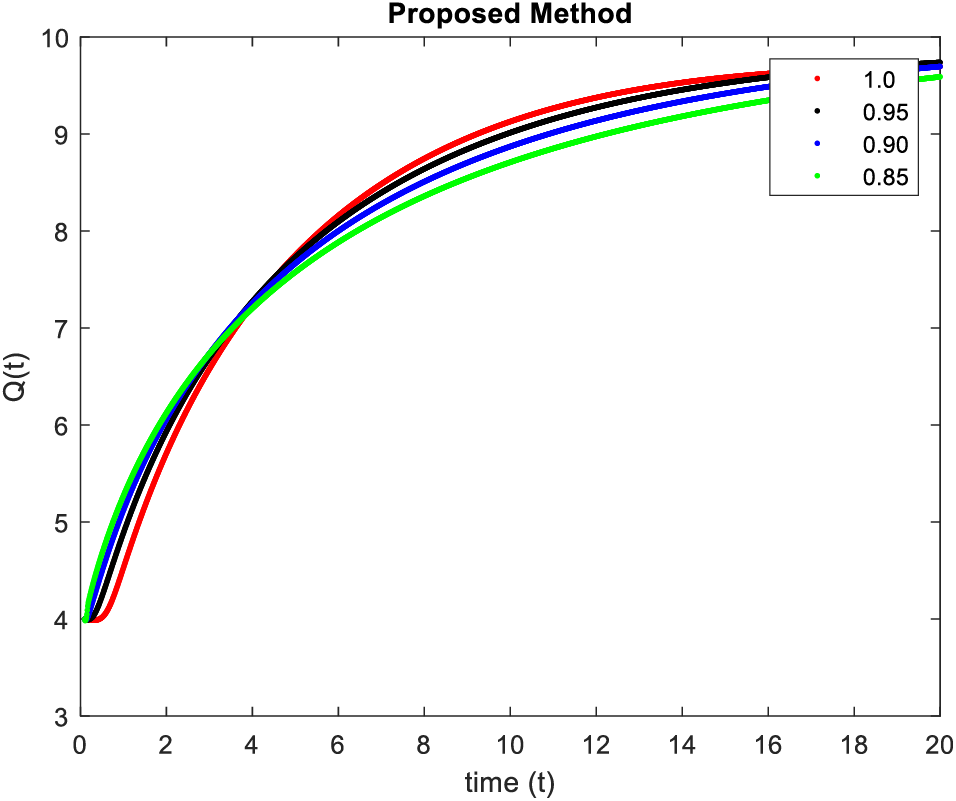
Figure 4: Results of
In Figs. 5–8, simulations were obtained by fractal fractional method. It is noted that physical procedures are far better explained using the fractional order derivatives which are the most notable and sustainable component compared to the classical-order case with order at 0.9. The behaviors of the dynamics found in the various fractional orders are shown in the form of numerical results that have been reported.
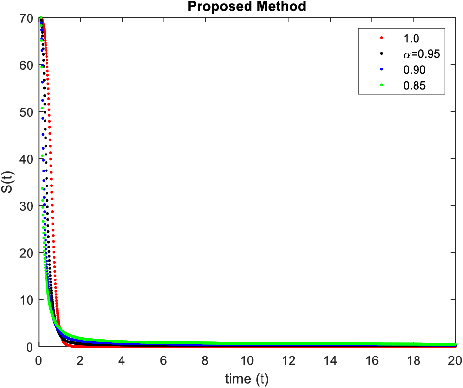
Figure 5: Results of
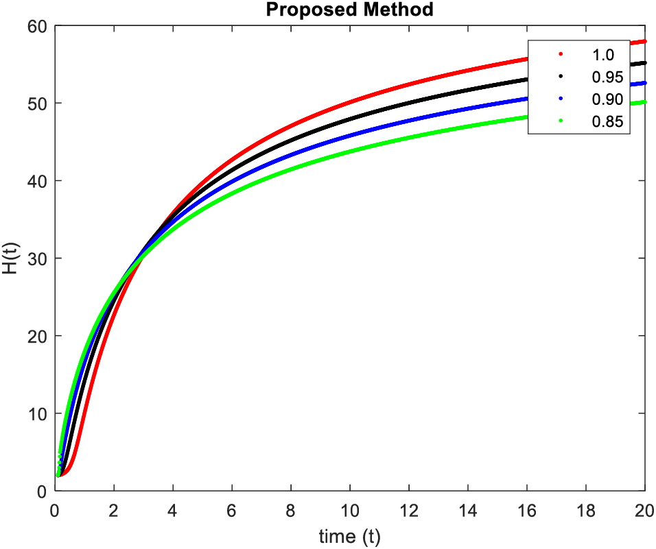
Figure 6: Results of
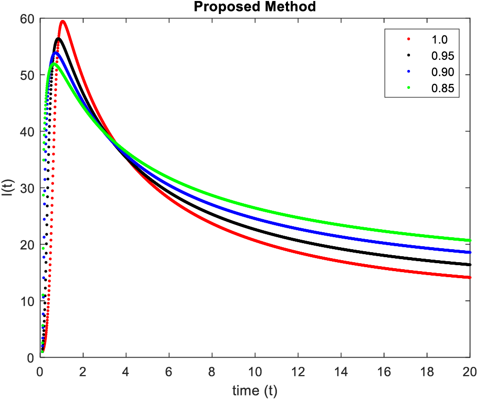
Figure 7: Results of
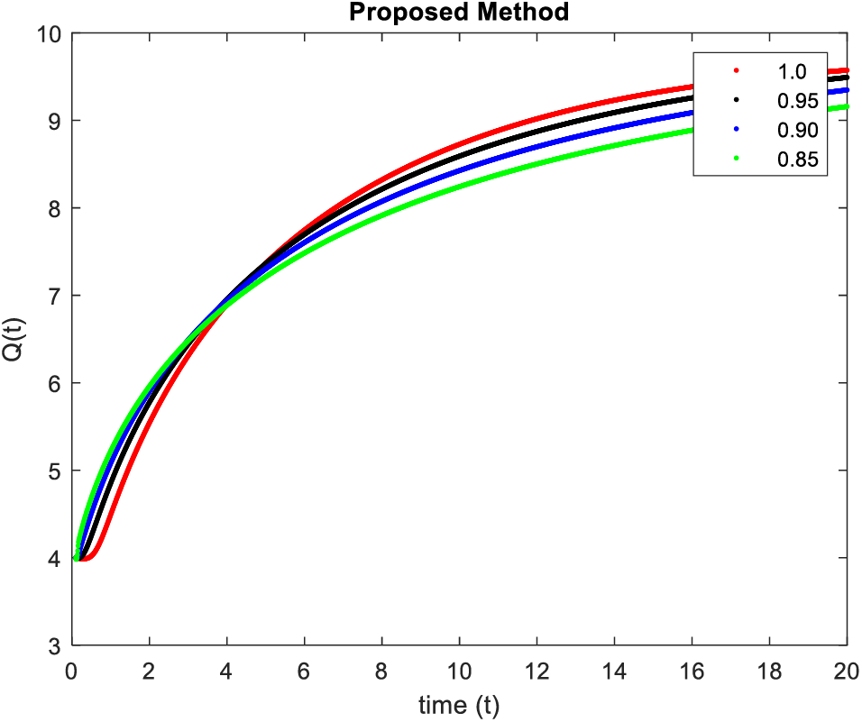
Figure 8: Simulation of
In Figs. 9–12, simulations were obtained by fractal fractional method. It is noted that physical procedures are far better explained using the fractional order derivatives which are the most notable and sustainable component compared to the classical-order case with order at 0.8. The behaviors of the dynamics found in the various fractional orders are shown in the form of numerical results that have been reported.
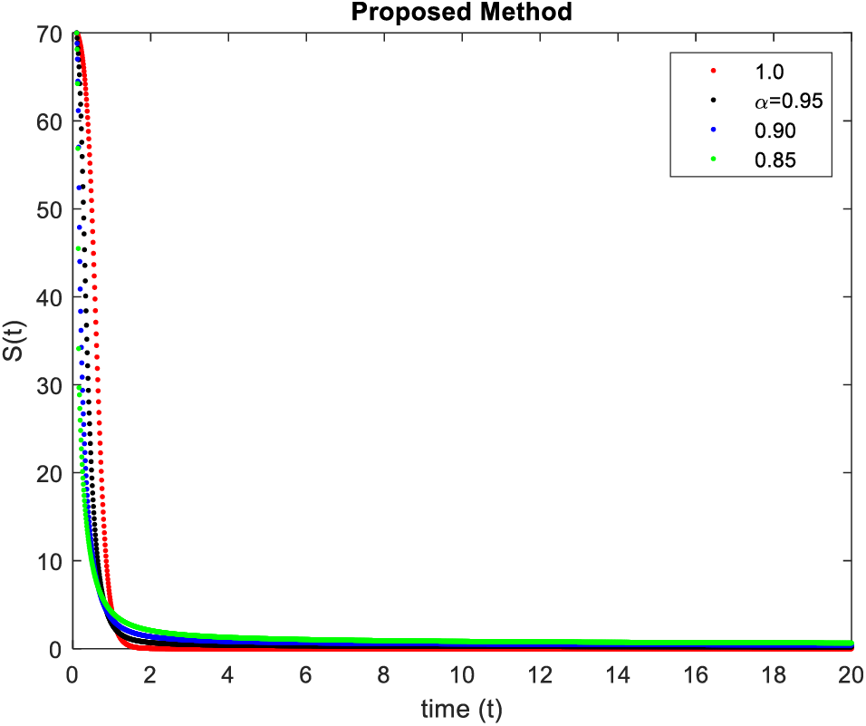
Figure 9: Results of
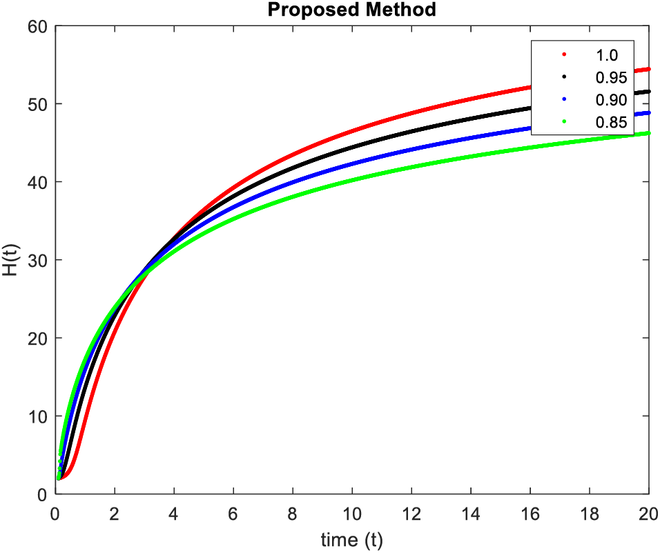
Figure 10: Results of
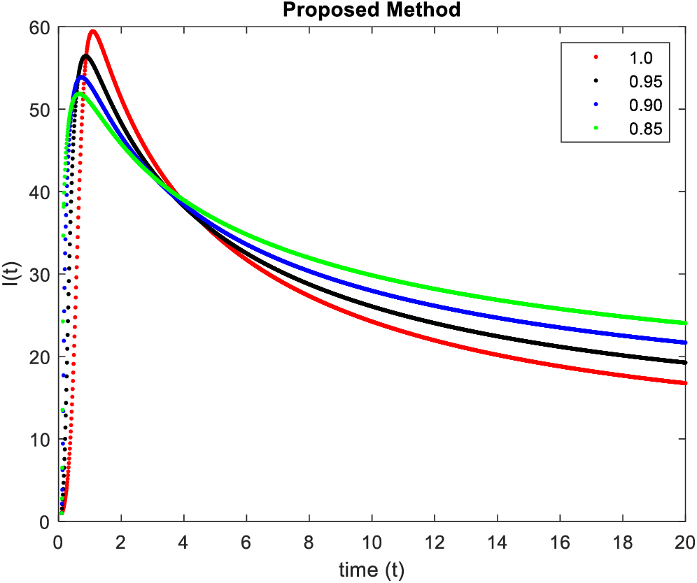
Figure 11: Results of
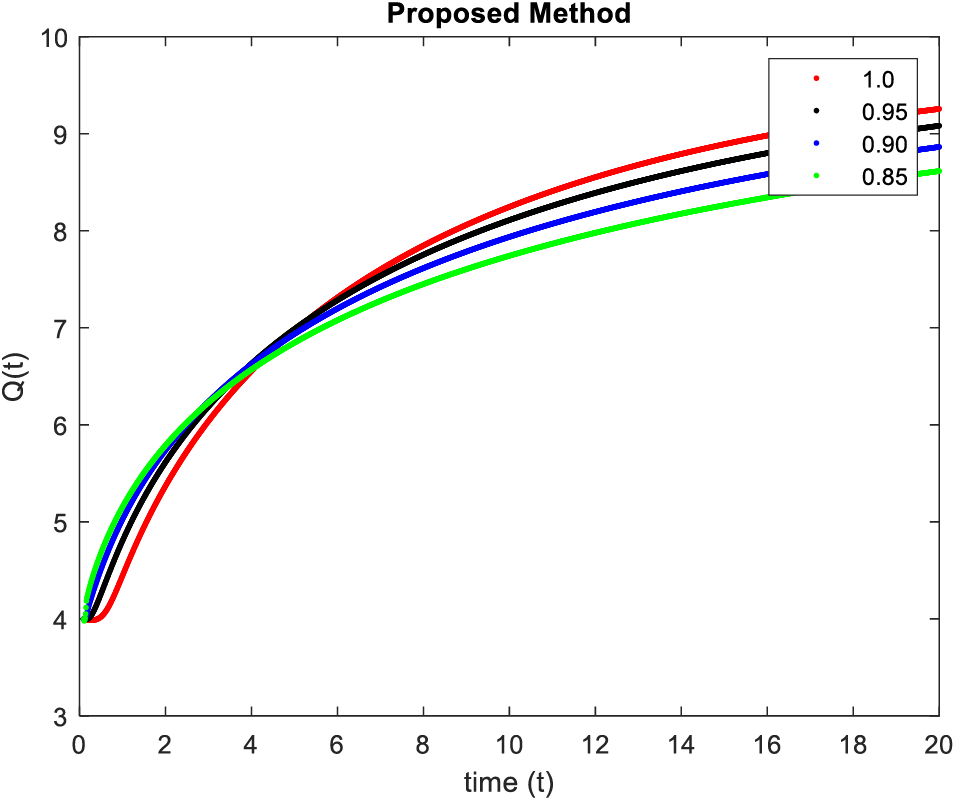
Figure 12: Results of
In this paper, the fractal-fractional differential equation model for COVID-19 disease has been investigated with fractal fractional operator. The steady state and fundamental characteristics of the model equilibria are investigated. Fixed point theory is used to demonstrate in detail the existence and uniqueness of solutions for the model with FFM derivative. The Ulam-Hyers technique is used to conduct the stability analysis of the system which fulfills all properties. The two-step fractional Lagrange polynomial approach with FFM derivative is used to generate the model’s numerical solution. The numerical simulations are obtained and briefly described by choosing various values of the fractional order and dimension. We applied very effective numerical techniques to obtain the solutions of the model. We analyzed our obtained results and concluded that they are effective for the proposed model. Some theoretical results were also discussed for the model. This model turns out to be quite trustworthy when precise estimations of transmission structures are provided in real-time. The new suggested improvement will shed some modeling-related light on problems with and without singularity at the origin.
The analysis of the following problems forms further directions of research and developments: creating and exploring families of other epidemiological models based on fractal-fractional differential equations for diseases; the exploration of distinctions, taking into account the types of distinctions between fractional models; creating the output information for subsequent methodological recommendations, for diseases expansions analysis and for anti-diseases interventions plans.
Acknowledgement: The authors would like to acknowledge the Lucian Blaga University of Sibiu & Hasso Plattner Foundation’s research grant.
Funding Statement: Lucian Blaga University of Sibiu & Hasso Plattner Foundation Research Grants LBUS-IRG-2020-06.
Author Contributions: Conceptualization, M.F., A.A. and M.S.H.; Methodology, M.F., A.A. and M.S.H.; Formal analysis, M.F., A.A., M.S.H., A.B. and L.G.; Investigation, M.F., A.A. and M.S.H.; Supervision, A.B. and L.G.; Project administration, A.B.; Funding acquisition, A.B. All authors have read and agreed to the published version of the manuscript.
Availability of Data and Materials: Not applicable.
Conflicts of Interest: The authors declare that they have no conflicts of interest to report regarding the present study.
References
1. Jasper, F. W. C. (2020). Genomic characterization of the 2019 novel human-pathogenic coronavirus isolated from patients with acute respiratory disease in Wuhan, Hubei, China. Emerging Microbes & Infections, 9(1), 221–236. [Google Scholar]
2. World Health Organization (WHO). https://www.who.int/emergencies/diseases/novel-coronavirus-2019/technical-guidance2020 [Google Scholar]
3. Lu, H., Stratton, C. W., Tang, Y. W. (2020). Outbreak of pneumonia of unknown etiology in Wuhan, China: The mystery and the miracle. Journal of Medical Virology, 92, 401. [Google Scholar] [PubMed]
4. Ji, W., Wang, W., Zhao, X., Zai, J., Li, X. (2020). Homologous recombination within the spike glycoprotein of the newly identified coronavirus may boost cross-species transmission from snake to human. Journal of Medical Virology, 94(4), 433–440. [Google Scholar]
5. World Health Organization (2021). Coronavirus Disease 2019 (COVID-19Situation Report. [Google Scholar]
6. Alnaser, W. E., Abdel-Aty, M., Al-Ubaydli, O. (2020). Mathematical prospective of coronavirus infections in Bahrain, Saudi Arabia and Egypt. Information Sciences Letters, 9(1), 51–64. [Google Scholar]
7. Ming, W., Huang, J. V., Zhang, C. J. P. (2020). Breaking down of the healthcare system: Mathematical modelling for controlling the novel coronavirus (2019-nCoV) outbreak in Wuhan, China. https://doi.org/10.1101/2020.01.27.922443 [Google Scholar] [CrossRef]
8. Nesteruk, I. (2020). Statistics-based predictions of coronavirus epidemic spreading in Mainland China. Innovative Biosystems and Bioengineering, 4(1), 13–18. [Google Scholar]
9. Kucharski, A. J., Russell, T. W., Diamond, C., Liu, Y., Edmunds, J. et al. (2020). Early dynamics of transmission and control of COVID-19: A mathematical modelling study. The Lancet Infectious Diseases, 20(5), 553–558. [Google Scholar] [PubMed]
10. Liu, Y., Gayle, A. A., Wilder-Smith, A., Rocklöv, J. (2020). The reproductive number of COVID-19 is higher compared to SARS coronavirus. Journal of Travel Medicine, 27(2). https://doi.org/10.1093/jtm/taaa021 [Google Scholar] [PubMed] [CrossRef]
11. Arif, M. S., Abodayeh, K., Ejaz, A. (2023). Computational modeling of reaction-diffusion COVID-19 model having isolated compartment. Computer Modeling in Engineering & Sciences, 135(2), 1719–1743. https://doi.org/10.32604/cmes.2022.022235 [Google Scholar] [PubMed] [CrossRef]
12. Raza, A., Baleanu, D., Khan, Z. U., Mohsin, M., Ahmed, N. et al. (2023). Stochastic analysis for the dynamics of a poliovirus epidemic model. Computer Modeling in Engineering & Sciences, 136(1), 257–275. https://doi.org/10.32604/cmes.2023.023231 [Google Scholar] [PubMed] [CrossRef]
13. Xu, C., Farman, M., Hasan, A., Akgul, A., Zakarya, M. et al. (2022). Lyapunov stability and wave analysis of COVID-19 omicron variant of real data with fractional operator. Alexandria Engineering Journal, 61(12), 11787–11802. [Google Scholar]
14. Toufik, M., Atangana, A. (2017). New numerical approximation of fractional derivative with non-local and non-singular kernel: Application to chaotic models. European Physical Journal Plus, 132, 444. [Google Scholar]
15. Akgul, E. K. (2019). Solutions of the linear and nonlinear differential equations within the generalized fractional derivatives. Chaos, 29(2), 023108. [Google Scholar] [PubMed]
16. Atangana, A., Akgul, A. (2020). Can transfer function and bode diagram be obtained from Sumudu transform. Alexandria Engineering Journal, 59, 1971–1984. [Google Scholar]
17. Farman, M., Saleem, M. U., Imtiaz, A. S., Tabassm, M. F., Akram, S. et al. (2020). A control of glucose level in insulin therapies for the development of artificial pancreas by atangana baleanu fractional derivative. Alexandria Engineering Journal, 59, 2639–2648. [Google Scholar]
18. Hashemi, M. S. (2018). Some new exact solutions of (2+1) dimensional nonlinear Heisenberg ferromagnetic spin chain with the conformable time fractional derivative. Optical and Quantum Electronics, 50(2), 1–11. [Google Scholar]
19. Hashemi, M. S., Baleanu, D. (2020). Lie symmetry analysis of fractional differential equations. New York: CRC Press. [Google Scholar]
20. Kheybari, S., Darvishi, M. T., Hashemi, M. S. (2019). Numerical simulation for the space-fractional diffusion equations. Applied Mathematics and Computation, 348, 57–69. [Google Scholar]
21. Hashemi, M. S., Inc, M., Hajikhah, S. (2021). Generalized squared remainder minimization method for solving multi-term fractional differential equations. Nonlinear Analysis: Modelling and Control, 26(1), 57–71. [Google Scholar]
22. Khalid, N., Abbas, M., Iqbal, M. K., Singh, J., Ismail, A. I. M. (2020). A computational approach for solving time fractional differential equation via spline functions. Alexandria Engineering Journal, 59(5), 3061–3078. [Google Scholar]
23. Khalid, N., Abbas, M., Iqbal, M. K. (2019). Non-polynomial quintic spline for solving fourth-order fractional boundary value problems involving product terms. Applied Mathematics and Computation, 349, 393–407. [Google Scholar]
24. Majeed, A., Kamran, M., Abbas, M., Misro, M. Y. B. (2021). An efficient numerical scheme for the simulation of time-fractional nonhomogeneous Benjamin-Bona-Mahony-Burger model. Physica Scripta, 96(8), 084002. [Google Scholar]
25. Farman, M., Hasan, A., Sultan, M., Ahmad, A., Akgül, A. et al. (2023). Yellow virus epidemiological analysis in red chili plants using Mittag-Leffler kernel. Alexandria Engineering Journal, 66, 811–825. [Google Scholar]
26. Hashemi, M. S., Inc, M., Kilic, B., Akgul, A. (2016). On solitons and invariant solutions of the magneto-electro-elastic circular rod. Waves in Random and Complex Media, 26(3), 259–271. [Google Scholar]
27. Khan, M. A., Atangana, A. (2020). Modeling the dynamics of novel coronavirus (2019-nCoV) with fractional derivative. Alexandria Engineering Journal, 59(4), 2379–2389. [Google Scholar]
28. Atangana, A., Bonyah, E., Elsadany, A. A. (2020). A fractional order optimal 4D chaotic financial model with mittag-leffler law. Chinese Journal of Physics, 65, 38–53. [Google Scholar]
29. Aslam, M., Farman, M., Akgul, A., Sun, M. (2021). Modeling and simulation of fractional order COVID-19 model with quarantined-isolated people. Mathematical Method in Applied Sciences, 44(8), 6389–6405. [Google Scholar]
30. Farman, M., Ahmad, A., Akgul, A., Saleem, M. U., Naeem, M. et al. (2021). Epidemiological analysis of the coronavirus disease outbreak with random effects. Computer, Material & Continua, 67(3), 3215–3227. [Google Scholar]
31. Aslam, M., Farman, M., Akgul, A., Ahmad, A., Sun, M. (2021). Generalized form of fractional order COVID-19 model with Mittag-Leffler kernal. Mathematical Method in Applied Sciences, 44(11), 8598–8614. [Google Scholar]
32. Farman, M., Aslam, M., Akgul, A., Ahmad, A. (2021). Modeling of fractional order COVID-19 epidemic model with quarantine and social distancing. Mathematical Method in Applied Sciences. https://doi.org/10.1002/mma.7360 [Google Scholar] [PubMed] [CrossRef]
33. Farman, M., Akgul, A., Ahmad, A., Baleanu, D., Saleem, M. U. (2021). Dynamical transmission of coronavirus model with analysis and simulation. Computer Modeling in Engineering & Sciences, 127(2), 753–769. https://doi.org/10.32604/cmes.2021.014882 [Google Scholar] [PubMed] [CrossRef]
34. Ivorra, B., Ferrández, M. R., Vela-Pérez, M., Ramos, A. (2020). Mathematical modeling of the spread of the coronavirus disease 2019 (COVID-19) taking into account the undetected infections. the case of China. Communications in Nonlinear Science and Numerical Simulation, 88, 105303. [Google Scholar] [PubMed]
35. Kanno, R. (1998). Representation of random walk-in fractal space-time. Physica A: Statistical Mechanics and its Applications, 248, 165–175. [Google Scholar]
36. Atangana, A., Qureshi, S. (2019). Modelling attractors of chaotic dynamical systems with fractal-fractional operators. Chaos, Solitons & Fractals, 123, 320–337. [Google Scholar]
37. Chen, W., Sun, H., Zhang, X., Korosak, D. (2010). Anomalous diffusion modeling by fractal and fractional derivatives. Computers & Mathematics with Applications, 59(5), 1754–1758. [Google Scholar]
38. Atangana, A. (2017). Fractal-fractional differentiation and integration: Connecting fractal calculus and fractional calculus to predict complex system. Chaos, Solitons & Fractals, 102, 396–406. [Google Scholar]
39. Ahmad, S., Ullah, A., Al-Mdallal, Q. M., Khan, H., Shah, K. et al. (2020). Fractional order mathematical modeling of COVID-19 transmission. Chaos, Solitons & Fractals, 139, 110256. [Google Scholar]
40. Tanrıverdi, T., Mcleod, J. B. (2010). The Fanno model for turbulent compressible flow. Journal of Differential Equations, 249(12), 2955–2963. [Google Scholar]
41. Khan, M. A. (2021). The dynamics of dengue infection through fractal-fractional operator with real statistical data. Alexandria Engineering Journal, 60(1), 321–336. [Google Scholar]
42. Ahmad, S., Ullah, A., Abdeljawad, T., Akgül, A., Mlaiki, N. (2021). Analysis of fractal-fractional model of tumor-immune interaction. Results in Physics, 25, 104178. [Google Scholar]
43. Hashemi, M. S. (2020). A novel approach to find exact solutions of fractional evolution equations with non-singular kernel derivative. Chaos, Solitons & Fractals, 152, 111367. [Google Scholar]
44. Bucur, A., Guran, L., Petrusel, A. (2009). Fixed point theorems for multivalued operators on a set endowed with vector-valued metrics and applications. Fixed Point Theory, 1, 19–34. [Google Scholar]
45. Rus, I. A., Petrușel, A., Sîntămărian, A. L. (2001). A data dependence of the fixed point set of multivalued weakly Picard operators. Studia Universitatis Babeș-Bolyai Mathematica, 46(2), 111–121. [Google Scholar]
46. Ahmad, S., Owyed, S., Abdel-Aty, A. H., Mahmoud, E. E., Shah, K. et al. (2021). Mathematical analysis of COVID-19 via new mathematical model. Chaos, Solitons & Fractals, 143, 110585. [Google Scholar]
Cite This Article
 Copyright © 2024 The Author(s). Published by Tech Science Press.
This work is licensed under a Creative Commons Attribution 4.0 International License , which permits unrestricted use, distribution, and reproduction in any medium, provided the original work is properly cited.
 Downloads
 Citation Tools