Construction of a Computational Scheme for the Fuzzy HIV/AIDS Epidemic Model with a Nonlinear Saturated Incidence Rate

1  Introduction

Epidemiology is the branch that offers predictions against infectious diseases, their presence, and control among a given population. It explains the factors governing infection spread and provides a suitable precautionary measure adapted for its control. Therefore, one can say that epidemiology is the branch that improves the healthcare system by regulating disease spread [1]. In 1981, the USA was the first country to report early cases of HIV (a retrovirus) among transgender people, plotting it as a life-threatening ailment. To date, 25 million deaths have been reported, with 14,000 new cases/day forming a nightmare with no cure as no vaccine has yet been prepared. It requires 6 months to 15 years for an individual to become completely susceptible to HIV and reveal the symptoms.

On the other hand, the virus severely disrupts the CD4+ T-cells, affecting the autoimmunity system of cells. Ultimately, individuals lacking immunity became vulnerable to even minute diseases like influenza, leading them straight to death. The routes for HIV movement are unprotected sexual intercourse along with contaminated syringes, needles, and blood, which may infect the person when in use. Blood containing HIV, when transferred through vertical transmissions [2], could be fatal for a receiver.

Mathematics has given researchers enormous tools to build the epidemiology of HIV/AIDS and understand the involvement of variable factors contributing to the epidemic. Three approaches to the population-based study of the HIV/AIDS epidemic were made by Zafar et al. [3]. The Adams-Bashforth Moulton method, Grunwald Letnikov approach, and Grunwald Letnikov approach with binomial coefficients. In this study, the stability if Ro<1 and if Ro>1 and disability are discussed along with endemic equilibrium. A delayed fractional-order SIR model with saturated incidence and treatment functions was investigated by Wang et al. [4].

A fuzzy differential equation is commonly used to omit uncertainty modeling a dynamic system. Such a system may involve cell growth and the dynamic of population, tumor growth, and nuclear disintegration under uncertainty. The transition of HIV to AIDS can be modeled using a fuzzy transference rate correlated with the viral load and CD4+ T-cells level by rule bases [5]. Several drugs have been designed that are optimal for drug therapy and prescribed to HIV patients. Considering the drug therapy, several questions have been asked about the best medicinal therapy for the HIV patient, although the therapeutic period is confined. The answer lies in the traditional differential equation, which efficiently describes the interaction between HIV and an infective individual’s immune system. This equation provides an appropriate optimal control on the system of equations by a suitable medicine program [6].

Individuals carrying HIV depicted variable levels of their immune system regarding the number of immunity cells vs. concentration of virus inside the body during a virus attack. This could be modeled using mathematical modeling that interprets the ratio between HIV and immune cells. Perelson et al. in [7] elaborated on three state variables, i.e., healthy CD4+ T-cells, infected CD4+ T-cells, and viruses, and created the basis of a simple mathematical model for HIV. Complexity arises when considering other variables like cytotoxic T lymphocytes and macrophages, as reported by [8]. Ambiguity in the given publication arises due to an unclarified uncertainty description without interpreting fuzzy parameters. The major concern of this paper is to focus on uncertain parameters and halt them using the fuzzy equation in preparation for the HIV model.

Hukuhara derivative [9] was the pioneer who suggested the concept of differentiability for fuzzy mappings about the fuzzy differential equation. Time revealed that the fuzzy differential equation used by the Hukuhara derivative could be termed fuzzier and possesses different characters compared to a crisp solution [10]. To remove this obstacle, another strong variable, fuzzy-number-valued functions, was derived, which exclusively generalized differentiability as mentioned in [11–14].

The simplest are first-order fuzzy differential equations that as many applications. Whereas such simplest equation creates hurdles under different fuzzy differential equation concepts, i.e., the behavior of solutions is different (based on interpretation). Several researchers have utilized first-order fuzzy linear equations, as mentioned in [11]. Under the umbrella of the generalized differentiability notion, the author proposed a general form of the solutions to the first-order fuzzy differential equations with crisp coefficients. Recently operator approach has been proposed for solving first- and second-order linear fuzzy differential equations under strongly generalized differentiability [12]. Boundary value conditions have been introduced to the impulses [13]. A first-order linear fuzzy differential equation’s explicit solutions are found by calculating them on each level set and proving their existence and uniqueness. They are using the generalized Euler approximation approach. The numerical solution of the fuzzy differential equation under generalized differentiability has been studied in [14]. A generalization of Hukuhara’s differentiability for interval-valued functions has been introduced in [15]. Under this sort of differentiability, interval differential equations have local existence and uniqueness.

Linear fuzzy differential dynamical systems with complex number representation of level sets and solutions derived under this representation were the focus of [16], which focused on linear fuzzy differential dynamical systems with initial conditions defined by a fuzzy number vector. When solving linear differential dynamical systems, including fuzzy matrices, it is helpful to keep this in mind, but [17] goes one step further by providing solutions to these systems using fuzzy matrices in addition to those provided by [18].

This publication provided sufficient information for the existence of equilibrium and global stability concerning the endemic and infection-free medium by formulating suitable Lyapunov functions. Fractional SEIR epidemic models and fractional differential equations were examined by Almeida [19] in an attempt to understand the dynamics of specific epidemics. Carvalho et al. developed a fractional-order model of HIV/HCV coinfection to understand better how the HIV viral load affects the coinfection [20]. Their study was confined to providing a numeric of individuals suffering from various infections like HIV, HCV, dengue fever, and many others. However, results revealed that the HIV viral load impacts remarkably on the harshness of the HCV infection, and the treatment efficacy is dominated by the natural progression of HCV against HIV/HCV coinfection. Using a multi-patch HIV/AIDS epidemic model with fractional-order derivatives, Kheiri et al. [21] studied the effect of human drive on HIV/AIDS pandemic propagation among patches. The major objective of the study was to bring the basic reproduction number Ro of the model to observe local and global stability of the equilibrium based on Ro values. Fractional optimal control brings the system towards stability by making Ro<1 and disability when Ro>1, and hence proved that the endemic equilibrium is unique and globally asymptotically stable beside the presentation of state and co-state equation as left fractional derivatives.

The model formulated by [21] comprised time-dependent control to minimize the spread of HIV/AIDS and the derived fractional optimal control that varies the fractional order of the disease spread. Nowadays, plenty of literature on fractional-order models of HIV disease dynamics reveals the engagement of mathematical techniques. Such techniques solve the models and the disease dynamics (HIV) spread [22,23]. Studies focused on fractional-order modeling can be seen in the literature [24–26] and references therein. The most significant application of fractional order derivative is modeling infectious disease, vibration equations [27,28], and much more.

Moreover, massive optimal control theory applications have made it applicable in several fields of pure and applied sciences [29]. The theory of linear systems has been extensively worked on [30]. Contrary, the theory of nonlinear optimal control (OCP) needed a thorough description and further analysis [31,32]. The modal series method and eigenvalue decomposition technique were used by Jajarmi et al. [33] to illustrate a class of nonlinear optimal control problems and convergence analysis. Jajarmi et al. [34] investigated the optimal control of time-varying delay systems with persistent matched external disturbances. The uniqueness of their study, which made the whole working thing interesting, is the conversion of the disturbed original time-delay model into an augmented system without any disturbance. A quadratic performance index was chosen for the enhanced system to establish an undisturbed time-delay optimum control issue. Two-point boundary value problems drive to advance and delay optimality criteria. An iterative algorithm for solving the latter advance-delay boundary value problem with a new iterative technique was also offered. To approximate the solution of the HIV infection of CD4+ T-cells model, the authors of [35] employed the continuous Galerkin-Petrov method (cGP(2)-method). Different clinical parameters’ effects on the model are discussed and analyzed. In the study [36], we applied a Legendre wavelet collocation scheme to an HIV infection model and compared our results to those found elsewhere. The results show how accurate and useful the proposed method is for estimating the HIV model’s solutions. The purpose of the research presented in [37] was to create a new fuzzy fractional model for the human liver. This model would incorporate the ABC fractional differentiability, which is also referred to as the ABC gH-differentiability. It would be based on the generalized Hukuhara derivative. Using the gH-differentiability of Caputo fractional order, this study [38] developed and analyzed a robust double-parametric analytical approach for the nonlinear fuzzy fractional KdV equation (FFKdVE). With the time-dependent variable of carbon flux in the atmosphere, carbon flux in soil, and the carbon flux of animals and plants, the dynamical behaviors and mathematics of the fractional order atmosphere-soil-land plant carbon cycle system were studied in [39].

This study concerns a fuzzy epidemic model comprising five compartments: Susceptible, exposed, unaware, infective, aware, and recovered. The fuzzy-based interaction parameters are defined and further used in the model. The fuzzy parameters are split into three parts that discuss the unsuccessful, successful, and fully successful meetings of infective with susceptible. If the value of the fuzzy parameter falls between 0 and 1, then a higher value corresponds to higher chances of successful interaction of infective with susceptible. So, two fuzzy parameters in a model provide nine different cases because each fuzzy parameter is divided into three parts. The discussions related to three cases exist in this study, but the remaining cases can be discussed similarly. In addition, a numerical scheme is established for three of the discussed cases. The numerical scheme has the advantage over some existing classical schemes in determining conditions for a positive solution. The numerical scheme is established on three time levels, so either a different scheme is adopted, or some initial guess is chosen for the second time level. In this work, the forward Euler scheme is chosen for finding a solution at the second time level. Since the given scheme and existing forward Euler schemes are conditionally stable, both require suitable step sizes for obtaining a convergent solution. Among existing finite difference schemes for solving differential equations, a non-standard finite difference method has been chosen by various researchers for solving epidemic models. The non-standard finite difference scheme has been constructed on two-time levels. It is unconditionally stable and provides surety to get positive solutions for some of the existing epidemic models. But, the scheme has its drawback: it does not achieve first-order accuracy in the obtained solution. So, the solution obtained by a non-standard scheme is doubtful unless the proper step size is chosen. The scheme constructed in this work has the advantage over the non-standard scheme due to the order of accuracy. In addition, the constructed scheme has an advantage over the forward Euler method in terms of enlarged stability region, but the constructed scheme is conditionally stable.

2  Fuzzy Epidemic Model

Before starting the mathematical modeling and analysis of the fuzzy epidemic model, some basic definitions are given.

2.1 Fuzzy Subset [40]

A fuzzy subset of a Universe X is denoted by the function Pf(x):X→[0,1] where Pf(x) is a membership function representing the degree of membership of element x in the fuzzy set f.

2.2 Fuzzy Number

A fuzzy number is a generalization of a regular real number. It refers to a connected set of potential values instead of just one specific value, where each potential value weights 0 and 1. The membership function is the name of this weight. Consequently, a convex, normalized fuzzy set of the real line is a particular instance of a fuzzy number.

2.3 Triangular Fuzzy Number [40]

The number f=(a,b,c) is a triangular fuzzy number if its membership function is denoted by:

Pf(x)={0,x≤ax−ab−a,a<x≤bx−cb−c,b<x≤c0,c≤x(1)

where a≤b≤c.

2.4 Trapezoidal Fuzzy Number [40]

The number f=(a,b,c,d) is called a trapezoidal fuzzy number if its membership function is defined as:

μf(x)={x−ab−a,a≤x≤b1,b≤x≤cd−xd−c,c<x≤d0,otherwise(2)

where a≤b≤c≤d.

2.5 Expected Value [41]

The expected value of a triangular fuzzy number (p,q,r) is given as:

E(f)=p+2q+r4.(3)

where p, q, and r are constants.

2.6 Fuzzy Basic Reproductive Number [41]

The fuzzy basic reproductive number of a triangular fuzzy number R0(u1,u2) is given by:

R0f=E[R0(u1,u2)].(4)

The deterministic model given in [42] is expressed as:

dSdt=Λ−S(β1I1+β2I2)−λS,(5)

dEdt=S(β1I1+β2I2)−(λ+σ)E,(6)

dI1dt=σE−(ρ+λ+θ)I1,(7)

dI2dt=θI1−(λ+ρ)I2.(8)

dRdt=ρ(I1+I2)−(d+λ)R.(9)

where S denotes the susceptible, E denotes the exposed, I1 denotes the infected but unaware, I2 represents the infected but aware, R denotes the recovered individuals, Λ denotes the recruited rate of susceptible, β1 is the rate of transmission from susceptible to infected but unaware, β2 denotes the transmission rate from susceptible to becoming infected but aware, λ is the natural death rate which is not related to acquired immune deficiency syndrome (AIDS), θ is the rate of unaware infective to becoming aware infectives, σ is the rate of exposed to become unaware infectives, ρ denotes the rate of transferring infective to those having AIDS, and d denotes the AIDS-related to the death rate.

Now, a fuzzy mathematical model with the incidence rate of AIDS is represented as:

dSdt=−S(β1(u1)I11+α1I1+β2(u2)I21+α2I2),(10)

dEdt=S(β1(u1)I11+α1I1+β2(u2)I21+α2I2)−σE,(11)

dI1dt=σE−(ρ+θ)I1,(12)

dI2dt=θI1−ρI2,(13)

dRdt=ρ(I1+I2)−dR,(14)

where β1(u1),β2(u2),σ,ρ,θ,d are positive constants. Let β1(u1) and β2(u2) denote the chances of transmission disease rate from susceptible to unaware infective and aware infective, respectively, β1(u1) and β2(u2) are defined as:

β1(u1)={0,u1<um,1u1−um,1u0,1−um,1,um,1<u1<u0,11,u0,1≤u1<uM,1(15)

β2(u2)={0,u2<um,2u2−um,2u0,2−um,1,um,2<u2<u0,21,u0,2≤u2<uM,2(16)

The β1(u) shows that a higher value of u1 produces higher β1(u1) which is greater than some minimum um,1. The transferring of disease from susceptible to infectives is ignorable if u1 is smaller than um,1. Also, the rate of transmission of disease from susceptible to infectives ones will be higher if u1 is greater than u0,1.

3  Mathematical Analysis

The equilibrium point of the model (10)–(13) will be found in this section.

3.1 Fuzzy Equilibrium Analysis

The system (10)–(13) has disease-free equilibrium points

E0(S0,E0,I10,I20)=E0(S0,0,0,0)(17)

3.2 Fuzzy Basic Reproductive Number

The first basic reproductive number of the deterministic model will be found. For doing so, the next-generation matrix approach is considered. According to this approach, the following matrices can be found:

ℱ(ψ)=[S(β1I11+α1I1+β2I21+α2I2)000],(18)

υ(ψ)=[σE−σE+(ρ+θ)I1−θI1+ρI2S(β1I11+α1I1+β2I21+α2I2)],(19)

where

ψ′=ℱ(ψ)−υ(ψ),(20)

and ψ=(E,I1,I2,S)T.

Since infected compartments are E,I1 and I2, so

F=[∂ℱP(E∘)∂ym]andV=[∂υP(E∘)∂ym]for1≤m,P≤3,(21)

F and V are given by

F=[σ00−σρ+θ00−ρ−θρ]andV=[σ00−σρ+θ00−ρ−θρ].(22)

The spectral radius of FV−1 gives the basic reproductive number, which is given as:

R0=ρβ1+β2(ρ+θ)ρ(ρ+θ).(23)

The fuzzy basic reproductive number is given by:

R¯0=ρβ(u1)+β2(u2)(ρ+θ)ρ(ρ+θ).(24)

Since there are three parts for each β1(u) and β2(u), so nine possible cases can be discussed. But in this work, only three will be discussed for convenience.

Case I: In this case u1<um,1 and u2<um,2 then β1(u1)=0=β2(u2), so R¯0 is given by:

R¯0=0.(25)

Case II: For this case, let um,1≤u1≤u0,1 and um,2≤u2≤u0,2, then

β1(u1)=u1−um,1u0,1−um,1andβ2(u2)=u2−um,2u0,2−um,2.

The fuzzy basic reproductive number is given by:

R¯0=ρβ1(u1)+β2(u2)(ρ+θ)ρ(ρ+θ).(26)

Case III: When u0,1<u1<uM,1 and u0,2<u2<uM,2 then β1(u1)=1=β2(u2) and so

R¯0=2ρ+θρ(ρ+θ).(27)

R0(u) can be expressed as:

R0(u1,u2)=(0,ρβ1(u1)+β2(u2)(ρ+θ)ρ(ρ+θ),2ρ+θρ(ρ+θ)),

where β1(u1)=u1−um,1u0,1−um,1 and β2(u2)=u2−um,2u0,2−um,2.

Given the definition of the expected value, R0f is expressed as:

R0f=E[R0(u1,u2)],

R0f=ρ(2β1(u1)+2β2(u2)+2)+θ(1+2β2(u2))4ρ(ρ+θ).(28)

3.3 Sensitivity Analysis

For a parameter S, the normalized forward parameter sensitivity index is given by:

ϕ(S)=SR0f∂R0f∂S.(29)

The sensitivity of parameters is given by:

ϕ(β1(u1))=β1(u1)R0f∂∂β1(u1)(ρ(2β1(u1)+2β2(u2)+2)+θ(1+2β2(u2))4ρ(ρ+θ))=2ρβ1(u1)ρ(2β1(u1)+2β2(u2)+2)+θ(1+2β2(u2))>0,(30)

ϕ(β2(u2))=β2(u2)R0f∂∂β2(u2)(ρ(2β1(u1)+2β2(u2)+2)+θ(1+2β2(u2))4ρ(ρ+θ))=β2(u2)(2ρ+2θ)ρ(2β1(u1)+2β2(u2)+2)+θ(1+2β2(u2))>0,(31)

ϕ(ρ)=ρR0f∂∂ρ(R0f)=−2(1+β1+β2)ρ2+(1+2β2)θ2+2ρ(θ+2β2θ)(ρ+θ)(2(1+β1+β2)ρ+θ+2β2θ)<0,(32)

ϕ(θ)=θR0f∂∂θ(R0f)=(1+2β1)ρθ(ρ+θ)(2(1+β1+β2)ρ+θ+2β2θ)<0.(33)

According to sensitivity analysis, β1(u1) and β2(u2) are sensitive parameters. The sensitive parameters and R0f have a direct relationship. By increasing sensitive parameters, R0f increases and vice versa. The insensitive parameters have an indirect relationship with R0f. It means that a decrease in insensitive parameters will increase R0f and vice versa.

3.4 Theorem

If R0≤1 and ρ2+2ρσ+ρθ+σθ>β1(u1)σ holds, then disease-free equilibrium point E0(S0,0,0,0) of the system (10)–(13) will be locally asymptotically stable.

Proof: For proving this theorem, eigenvalues for the Jacobian system (10)–(13) must have non-positive eigenvalues. For doing so, consider the Jacobian of the system (10)–(13) in the form of

[00−β1(u1)−β2(u2)0−σβ1(u1)β2(u2)0σ−ρ−θ000ρ+θ−ρ].(34)

Case I: When u1<um,1 and u2<um,2 then β1(u1)=0=β2(u2), so the Jacobian (34) can be written as:

J0=[00000−σ000σ−ρ−θ000ρ+θ−ρ].(35)

The eigenvalues of (35) are:

λ¯1=0,−ρ−θ,−ρ,−σ.(36)

Since all eigenvalues are negative, system (10)–(13) is stable for this case.

Case II: In this case, um,1≤u1<u0,1 and um,2≤u2<u0,2, then β1(u1)=u1−um,1u0,1−um,1 and β2(u2)=u2−um,2u0,2−um,2, and characteristic polynomial for (34) can be written as:

R(λ¯)=λ¯(λ¯3+a2λ¯2+a1λ¯+a0),(37)

where a0=−β1(u1)ρσ−β2(u2)ρσ+ρ2σ−β2(u2)σθ+ρσθ.

a1=ρ2−β1σ+2ρσ+ρθ+σθ

a2=2ρ+σ+θ

According to Routh Hurwitz’s criterion for cubic polynomials, the eigenvalues will lie in the left half plane, if and only if a0,a1,a2>0 and a1a2>a0.

The condition a2 is satisfied because all terms are positive. The condition a0>0 follows from R0≤1. For proving a1a2>a0, first the expression for a1a2−a0 will be found, which is given as:

a1a2−a0=2ρ3−β1(u1)ρσ+β2(u2)ρσ+4ρ2σ−β1(u1)σ2+2ρσ2+3ρ2θ−β1(u1)σθ+β2(u2)σθ+4ρσθ+σ2θ+ρθ2+σθ2.(38)

All terms in (38) are positive except for three terms. Now, the second inequality in the theorem statement will be utilized.

Since ρ2+2ρσ+ρθ+σθ>β1(u1)σ holds. From here, three more inequalities can be constructed as:

ρ3+2ρ2σ+ρ2θ+ρσθ>β1(u1)σρ,(39)

ρ2σ+2ρσ2+ρθσ+σ2θ>β1(u1)σ2,(40)

ρ2θ+2ρσθ+ρθ2+σθ2>β1(u1)σθ.(41)

By using inequalities (39)–(41) in (38), it can be shown that a1a2−a0>0. Therefore, all the conditions of the Routh Hurwitz criterion are satisfied, so eigenvalues lie in the left half plane.

Case III: When u1≥u0,1 and u2>u0,2 then β1(u1)=1=β2(u2), then it can be shown that eigenvalues are non-positive.

4  Numerical Scheme

A numerical scheme is presented for solving systems (10)–(13). The scheme will be constructed for the model’s first Eq. (10). For doing so, consider the discretized equation for Eq. (10) as:

Sn+1=(Sn−1+Sn)2+a¯1h[−Sn+1(β1(u1)I1n1+α1I1n+β2(u2)I2n1+α2I2n)],(42)

where h is step size and a¯1 will be determined later.

For finding a¯1 Taylor series expansions for Sn+1 and Sn−1 will be considered, which are given as follows:

Sn+1=Sn+h(dSdt)n+O(h2),(43)

Sn−1=Sn−h(dSdt)n+O(h2).(44)

Substituting Taylor series expansions (43) and (44) into Eq. (42) yields

Sn+h(dSdt)n=Sn−h(dSdt)n+a¯1h[−Sn(β1(u1)I1n1+α1I1n+β2(u2)I2n1+α2I2n)−h(dSdt)n(β1(u1)I1n1+α1I1n+β2(u2)I2n1+α2I2n)].(45)

Eq. (45) can be expressed as:

Sn+h(dSdt)n=Sn−h2(dSdt)n+a¯1h[(dSdt)n−h(dSdt)n(β1(u1)I1n1+α1I1n+β2(u2)I2n1+α2I2n)].(46)

Equating coefficients of Sn and h(dSdt)n on both sides of Eq. (46), it is obtained:

1=−12+a¯1(1−h(β1(u1)I1n1+α1I1n+β2(u2)I2n1+α2I2n)).(47)

The unknown a¯1 can be found as:

a¯1=3/21−h(β1(u1)I1n1+α1I1n+β2(u2)I2n1+α2I2n).(48)

Given Eqs. (48), (42) can be written as:

Sn+1=12(Sn−1+Sn)1+a¯1h(β1(u1)I1n1+α1I1n+β2(u2)I2n1+α2I2n).(49)

Similarly, the following equations can be obtained:

En+1=12(En−1+En)+Sn(β1(u1)I1n1+α1I1n+β2(u2)I2n1+α2I2n)a¯2h1+a¯2hσ,(50)

I1n+1=12(I1n−1+I1n)+a¯3hσ1+a¯3h(ρ+θ),(51)

I2n+1=12(I2n−1+I2n)+a¯4hθ1+a¯4hρ,(52)

where

a¯2=3/21−hσ,

a¯3=3/21−h(ρ+θ),

a¯4=3/21−hρ.

Case I: When u1<um,1 and u2<um,2 then β1(u1)=0=β2(u2) and Eqs. (49) and (50) can be written as:

Sn+1=12(Sn−1+Sn),(53)

En+1=12(En−1+En)1+a¯2hσ.(54)

where a¯2 is the same as given before. The rest of the difference equations for this case will be the same.

Case II: When um,1≤u1<u0,1 and um,2≤u2<u0,2 then β1(u1)=u1−um,1u0,1−um,1, and

β2(u2)=u2−um,2u0,2−um,2. The difference equation for this case is already given in (49)–(52).

Case III: When u0,1≤u1<uM,1 and u0,2≤u2<uM,2 then β1(u1)=1=β2(u2). Therefore, Eqs. (49) and (50) are expressed as:

Sn+1=12(Sn−1+Sn)1+a¯1h(I1n1+α1I1n+I2n1+α2I2n),(55)

En+1=12(En−1+En)+Sn(I1n1+α1I1n+I2n1+α2I2n)1+a¯2hσ.(56)

The rest of the equations will be the same as in this work.

4.1 Stability Analysis

For finding the stability conditions system of Eqs. (10)–(13) can be expressed as:

dHdt=(J1−J2)H,(57)

where J=J1−J2 and H=(S,E,I1,I2)T,J is the Jacobian of the system (10)–(13) evaluated at equilibrium points E0(1,0,0,0) and J1 & J2 are given as:

J1=[000000β1(u1)β2(u2)0σ0000ρ+θ0]andJ2=[00β1(u1)β2(u2)0σ0000ρ+θ0000ρ].

Discretizing Eq. (57) using the proposed scheme gives:

Hn+1=12(Hn−1+Hn)+bh(J1Hn−J2Hn+1),(58)

where b=32(I−hJ2)−1 and I is an identity matrix. Eq. (58) can be written as:

Hn+1=(I+bhJ2)−1(Hn+Hn−12+bhJ1Hn).(59)

The characteristic polynomial for Eq. (59) can be expressed as:

ω2−(I+bhJ2)−1(12I+bhJ1)ω+(I+bhJ2)−1I2=0.(60)

The scheme will be stable if the following condition holds:

|(1+bhλ¯2)−1(12+bhλ¯1)±(1+bhλ¯2)−2(12+bhλ¯1)2−2(1+bhλ¯2)−12|<1,(61)

where λ¯2 denotes the maximum eigenvalue of J2. For three cases, some entries of J1 and J2 will be changed, and the remaining proceeds will be the same.

5  Results and Discussions

The fuzzy epidemic model has been constructed in this work. The model comprised fuzzy parameters that can be more generalized than classical ones. These given fuzzy parameters depend on the quantities of the interaction of people. The interaction parameters are divided into three categories. Suppose the quantities for the interaction of infective with susceptible are less than some minimum number. In that case, none of the susceptible will shift to the category of exposed people. If the interaction of people falls in a specific range, then the classical model can be used in which different values of parameters can be chosen. If the interaction of people is greater than some number, then there will be a 100% chance that the susceptible will become an exposed individual. So, nine possible cases can be discussed based on these three cases for one parameter. But, in this work, only a few cases have been discussed, and the rest can be discussed similarly. The presented numerical scheme has been constructed for three cases with specific values of β1(u1) and β2(u2). The consistency of the numerical scheme has not been discussed. It can be proved by applying Taylor series expansions. But, since the order of accuracy of the proposed scheme is one, it is consistent. The convergence of the scheme mainly depends on the choice of parameters and the considered value of step size. The convergence of numerical solutions can be controlled by choosing a suitable step size. Since the presented scheme utilizes three grid points, a solution at the second grid point is required for employing the scheme. For this work, the forward Euler scheme has been employed on the second grid points, and the presented scheme has been employed for the rest of the grid points. Since the solution remains positive for some specific values of the parameters, any numerical scheme can be considered for those parameters. So, forward Euler can also be considered for finding numerical solutions to epidemic disease models. Also, forward Euler does not produce the conditions for getting the positive solution, but the presented scheme determines the conditions for checking the positivity of the solution.

Fig. 1 shows the effect of β1(u1) on susceptible and exposed people. The clear decay in the susceptible people can be seen, and little growth in the exposed people can be seen in Fig. 1. Since the increase in the β1(u1) leads to shifting the susceptible people to exposed people, so susceptible people will decrease, and exposed people will increase due to the entrance of susceptible into the category of exposed people. The effect of parameter α1 on susceptible and exposed people is deliberated in Fig. 2. The small increase in the susceptible people and dual behavior in exposed individuals can be seen in Fig. 2. The growth in α1 will decrease the interaction of susceptible and infective resulting in changes in the susceptible and exposed individuals. The influence of σ on infective people can be seen in Fig. 3. Both categories of infective have dual behavior by incrementing the parameter σ. The effect of σ on both types of infectives can be seen in particular intervals. Initially, both types of infectives rise, but with time, the rise in infectives people converts to decay. Fig. 4 shows the infective people with a variation of the parameter ρ. By incrementing ρ, decay in both types of infective people can be seen in Fig. 4. Since higher values of ρ show that more people have transferred to people who have AIDS. So, due to this fact, the number of infective decays. The effect of parameter σ on infective people can be seen in Fig. 5 for case 3 discussed in this work. Again, the dual behavior of aware and unaware infective can be seen in Fig. 5. The decay in the infective people by incrementing the parameter ρ for case 3 is displayed in Fig. 6. The variation of β2(u2) when β1(u1)=0 on susceptible and exposed people is displayed in Fig. 7. The decay in the susceptible people and escalation in the exposed people can be observed by looking at Fig. 7. The escalating values of the parameter β2(u2) will tend to shift the susceptible people to the category of exposed people, leading to decay in the susceptible people and growth in the exposed people. Since the model, in this case, does not consider the birth rate of susceptible people, and so the equilibrium point is fixed at E0(S0,0,0,0). The relationship between susceptible, exposed, and unaware infective can be seen in Fig. 8 without including the birth rate of susceptible people. Figs. 9–11 show the relationships of susceptible, exposed, and unaware infective people with different birth rates of susceptible people. Since choosing different birth rates of susceptible people, the equilibrium points of the system change, resulting in a different plot for the relationship between susceptible, exposed, and unaware infective.

Figure 1: Effect of parameter β1(u1) on susceptible and exposed people for case 2 using α1=0.1,α2=0.3,β2=0.5,σ=0.1,ρ=0.3,θ=0.5,N=50

Figure 2: Effect of parameter α1 on susceptible and exposed people for case 2 using β1=0.5,α2=0.3,β2=0.5,σ=0.1,ρ=0.3,θ=0.5,N=50

Figure 3: Effect of parameter σon unaware and aware infective people for case 2 using α1=0.5,α2=0.3,β2=0.5,β1=0.5,ρ=0.3,θ=0.5,N=50

Figure 4: Effect of parameter ρ on unaware and aware infective people for case 2 using α1=0.5,α2=0.3,β2=0.5,β1=0.5,σ=0.5,θ=0.5,N=50

Figure 5: Effect of parameter σ on unaware and aware infective people for case 3 using α1=0.5,α2=0.3,β2=1,β1=1,ρ=0.5,θ=0.5,N=50

Figure 6: Effect of parameter ρ on unaware and aware infective people for case 3 using α1=0.5,α2=0.3,β2=1,β1=1,σ=0.5,θ=0.5,N=50

Figure 7: Effect of parameter β2(u2) on susceptible and exposed people using α1=0.5,α2=0.3,σ=0.5,β1=0,ρ=0.5,θ=0.5,N=50

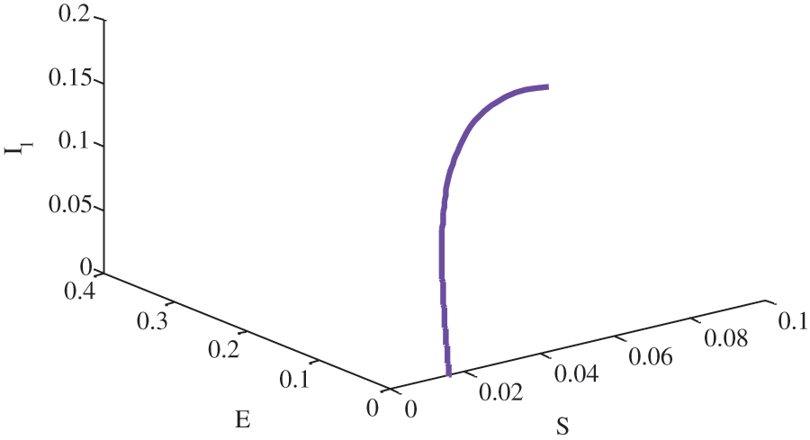
Figure 8: Relationship between susceptible, exposed and unaware infective people without birth rate of susceptible people using α1=0.5,α2=0.3,β2=1,β1=1,ρ=0.5,σ=0.5,θ=0.5,N=50

Figure 9: Relationship between susceptible, exposed and unaware infective people with a birth rate of 0.1 for susceptible people for case 3 using α1=0.5,α2=0.3,β2=1,β1=1,ρ=0.5,σ=0.5,θ=0.5,N=50

Figure 10: Relationship between susceptible, exposed and unaware infective people with a birth rate of 0.1 for susceptible people for case 2 using α1=0.5,α2=0.3,β2=1,β1=1,ρ=0.5,σ=0.5,θ=0.5,N=50

Figure 11: Relationship between susceptible, exposed and unaware infective people with a birth rate of 0.01 for susceptible people for case 2 using α1=0.5,α2=0.3,β2=1,β1=1,ρ=0.5,σ=0.5,θ=0.5,N=50

Table 1 shows the comparison of schemes for finding errors. Since the exact solution of the considered system is not available, a numerical solution is adopted. The Matlab solver ode45 obtains the numerical solution. Looking at Table 1, it can be concluded that the proposed scheme performs better than the existing non-standard finite difference method in most cases.

6  Conclusion

A fuzzy epidemic model has been proposed in this work. The model consists of five compartments. The fuzzy transmission rates have been defined in the model. The fuzzy transmission rate parameters have been divided into three parts based on three possibilities for the interaction of unaware and aware infective with susceptible people. The numerical scheme has been established for some fuzzy parameter cases. The concluding points can be expressed as:

•   The established scheme had an advantage over the existing forward Euler method in finding conditions for positive solutions.

•   Also, the constructed scheme produced less error than the existing NSFD method in small step sizes.

•   Susceptible people de-escalated, and exposed people escalated by incrementing fuzzy transmission parameters for unaware infective.

•   Both types of infectives were de-escalated by growth in the AIDS parameter.

•   Both types of infectives had dual behavior by raising transferring parameters from exposed to unaware infective.

•   The plots for relationships between susceptible, exposed, and infective converged to the model's equilibrium points with the susceptible people’s birth rate.

The established numerical scheme in this work can be employed in different branches of science and engineering to solve similar types of fuzzy differential equations. The findings of this study may lead to novel uses for the present method. Different types of theoretical and applied fuzzy differential equations might be amenable to the proposed technique. It can be put into action with little effort. After this study is over, the current method could be used in a variety of contexts [43, 44].

Acknowledgement: The authors wish to express their gratitude to Prince Sultan University for facilitating the publication of this article through the Theoretical and Applied Sciences Lab.

Funding Statement: The authors would like to acknowledge the support of Prince Sultan University for paying the article processing charges (APC) of this publication.

Author Contributions: Conceptualization, methodology, and analysis, writing—review and editing, Y.N.; funding ac-quisition, K.A.; investigation, Y.N.; methodology, M.S.A.; project administration, K.A.; resources, K.A.; supervision, M.S.A.; visualization, K.A.; writing—review and editing, M.S.A.; proofreading and editing, M.S.A. All authors have read and agreed to the published version of the manuscript.

Availability of Data and Materials: The manuscript included all required data and implementing information.

Conflicts of Interest: The authors declare that they have no conflicts of interest to report regarding the present study.

References

1. Dubey, P., Dubey, U. S., Dubey, B. (2018). Modeling the role of acquired immune response and antiretroviral therapy in the dynamics of HIV infection. Mathematics and Computers in Simulation, 144(1450), 120–137. [Google Scholar]

2. Dubey, B., Dubey, P., Dubey, U. S. (2015). Dynamics of an SIR model with nonlinear incidence and treatment rate. Applications and Applied Mathematics: An International Journal (AAM), 10(2), 5. [Google Scholar]

3. Zafar, Z. U. A., Rehan, K., Mushtaq, M. (2017). HIV/AIDS epidemic fractional-order model. Journal of Difference Equations and Applications, 23(7), 1298–1315. [Google Scholar]

4. Wang, X., Wang, Z., Huang, X., Li, Y. (2018). Dynamic analysis of a delayed fractional-order SIR model with saturated incidence and treatment functions. International Journal of Bifurcation and Chaos, 28(14), 1850180. [Google Scholar]

5. Zarei, H., Kamyad, A. V., Heydari, A. A. (2012). Fuzzy modelling and control of HIV infection. Computational and Mathematical Methods in Medicine, 2012, 1–17. [Google Scholar]

6. Zadeh, H. G., Nejad, H. C. (2012). Presentation of a fast solution for solving HIV-infection dynamics and chemotherapy optimization based on fuzzy: AVK method. Journal of AIDS and HIV Research, 4(3), 60–67. [Google Scholar]

7. Perelson, A. S., Neumann, A. U., Markowitz, M., Leonard, J. M., Ho, D. D. (1996). HIV-1 dynamics in vivo: Virion clearance rate, infected cell life-span, and viral generation time. Science, 271(5255), 1582–1586. [Google Scholar] [PubMed]

8. Hadjiandreou, M. M., Conejeros, R., Wilson, D. I. (2009). Long-term HIV dynamics subject to continuous therapy and structured treatment interruptions. Chemical Engineering Science, 64(7), 1600–1617. [Google Scholar]

9. Kaleva, O. (1987). Fuzzy differential equations. Fuzzy Sets and Systems, 24(3), 301–317. [Google Scholar]

10. Diamond, P., Kloeden, P. (1994). Metric spaces of fuzzy sets. Singapore: World Scientific. [Google Scholar]

11. Khastan, A., Nieto, J. J., Rodriguez-Lopez, R. (2011). Variation of constant formula for first order fuzzy differential equations. Fuzzy Sets and Systems, 177(1), 20–33. [Google Scholar]

12. Allahviranloo, T., Abbasbandy, S., Salahshour, S., Hakimzadeh, A. (2011). A new method for solving fuzzy linear differential equations. Computing, 92(2), 181–197. [Google Scholar]

13. Nieto, J. J., Rodríguez-López, R., Villanueva-Pesqueira, M. (2011). Exact solution to the periodic boundary value problem for a first-order linear fuzzy differential equation with impulses. Fuzzy Optimization and Decision Making, 10(4), 323–339. [Google Scholar]

14. Nieto, J. J., Khastan, A., Ivaz, K. (2009). Numerical solution of fuzzy differential equations under generalized differentiability. Nonlinear Analysis: Hybrid Systems, 3(4), 700–707. [Google Scholar]

15. Stefanini, L., Bede, B. (2009). Generalized Hukuhara differentiability of interval-valued functions and interval differential equations. Nonlinear Analysis: Theory, Methods & Applications, 71(3–4), 1311–1328. [Google Scholar]

16. Pearson, D. W. (1997). A property of linear fuzzy differential equations. Applied Mathematics Letters, 10(3), 99–103. [Google Scholar]

17. Ghazanfari, B., Niazi, S., Ghazanfari, A. G. (2012). Linear matrix differential dynamical systems with fuzzy matrices. Applied Mathematical Modelling, 36(1), 348–356. [Google Scholar]

18. Xu, J., Liao, Z., Nieto, J. J. (2010). A class of linear differential dynamical systems with fuzzy matrices. Journal of Mathematical Analysis and Applications, 368(1), 54–68. [Google Scholar]

19. Almeida, R. (2018). Analysis of a fractional SEIR model with treatment. Applied Mathematics Letters, 84(4), 56–62. [Google Scholar]

20. Carvalho, A. R., Pinto, C., Baleanu, D. (2018). HIV/HCV coinfection model: A fractional-order perspective for the effect of the HIV viral load. Advances in Difference Equations, 2018(1), 1–22. [Google Scholar]

21. Kheiri, H., Jafari, M. (2019). Stability analysis of a fractional order model for the HIV/AIDS epidemic in a patchy environment. Journal of Computational and Applied Mathematics, 346(7181), 323–339. [Google Scholar]

22. Kermack, W. O., McKendrick, A. G. (1933). Contributions to the mathematical theory of epidemics. III.—Further studies of the problem of endemicity. Proceedings of the Royal Society of London, 141(843), 94–122. [Google Scholar]

23. Ding, Y., Ye, H. (2009). A fractional-order differential equation model of HIV infection of CD4+ T-cells. Mathematical and Computer Modelling, 50(3–4), 386–392. [Google Scholar]

24. Khan, T., Ullah, R., Abdeljawad, T., Alqudah, M. A., Faiz, F. (2023). A theoretical investigation of the SARS-CoV-2 model via fractional order epidemiological model. Computer Modeling in Engineering & Sciences, 135(2), 1295–1313. https://doi.org/10.32604/cmes.2022.022177 [Google Scholar] [PubMed] [CrossRef]

25. Shah, K., Abdeljawad, T., Jarad, F., Al-Mdallal, Q. (2023). On nonlinear conformable fractional order dynamical system via differential transform method. Computer Modeling in Engineering & Sciences, 136(2), 1457–1472. https://doi.org/10.32604/cmes.2023.021523 [Google Scholar] [PubMed] [CrossRef]

26. Shah, K., Naz, H., Abdeljawad, T., Abdalla, B. (2023). Study of fractional order dynamical system of viral infection disease under piecewise derivative. Computer Modeling in Engineering & Sciences, 136(1), 921–941. https://doi.org/10.32604/cmes.2023.025769 [Google Scholar] [PubMed] [CrossRef]

27. Kumar, D., Singh, J., Al Qurashi, M., Baleanu, D. (2019). A new fractional SIRS-SI malaria disease model with application of vaccines, antimalarial drugs, and spraying. Advances in Difference Equations, 2019(1), 1–19. [Google Scholar]

28. Kumar, D., Singh, J., Baleanu, D. (2020). On the analysis of vibration equation involving a fractional derivative with Mittag-Leffler law. Mathematical Methods in the Applied Sciences, 43(1), 443–457. [Google Scholar]

29. Geering, H. P. (2007). Optimal control with engineering applications, vol. 113. Berlin: Springer. [Google Scholar]

30. Jia, W., He, X., Guo, L. (2017). The optimal homotopy analysis method for solving linear optimal control problems. Applied Mathematical Modelling, 45, 865–880. [Google Scholar]

31. Lin, H., Wei, Q., Liu, D. (2017). Online identifier-actor-critic algorithm for optimal control of nonlinear systems. Optimal Control Applications and Methods, 38(3), 317–335. [Google Scholar]

32. Almobaied, M., Eksin, I., Guzelkaya, M. (2018). Inverse optimal controller based on extended Kalman filter for discrete-time nonlinear systems. Optimal Control Applications and Methods, 39(1), 19–34. [Google Scholar]

33. Jajarmi, A., Baleanu, D. (2018). Optimal control of nonlinear dynamical systems based on a new parallel eigenvalue decomposition approach. Optimal Control Applications and Methods, 39(2), 1071–1083. [Google Scholar]

34. Jajarmi, A., Hajipour, M., Baleanu, D. (2018). A new approach for the optimal control of time-varying delay systems with external persistent matched disturbances. Journal of Vibration and Control, 24(19), 4505–4512. [Google Scholar]

35. Attaullah, R. D., Weera, W. (2022). Galerkin time discretization scheme for the transmission dynamics of HIV infection with non-linear supply rate. Journal of AIMS Mathematics, 6(6), 11292–11310. [Google Scholar]

36. Alyobi, S., Yassen, M. F. (2022). A study on the transmission and dynamical behavior of an HIV/AIDS epidemic model with a cure rate. AIMS Mathematics, 7(9), 17507–17528. [Google Scholar]

37. Verma, L., Meher, R. (2022). Study on generalized fuzzy fractional human liver model with Atangana–Baleanu–Caputo fractional derivative. The European Physical Journal Plus, 137(11), 1–20. [Google Scholar]

38. Verma, L., Meher, R., Avazzadeh, Z., Nikan, O. (2022). Solution for generalized fuzzy fractional Kortewege-de Varies equation using a robust fuzzy double parametric approach. Journal of Ocean Engineering and Science, 3(7), 109. https://doi.org/10.1016/j.joes.2022.04.026 [Google Scholar] [CrossRef]

39. Tanriverdi, T., Baskonus, H. M., Mahmud, A. A., Muhamad, K. A. (2021). Explicit solution of fractional order atmosphere-soil-land plant carbon cycle system. Ecological Complexity, 48(4), 100966. [Google Scholar]

40. Barros, L. C. D., Bassanezi, R. C., Lodwick, W. A. (2017). A first course in fuzzy logic, fuzzy dynamical systems, and biomathematics: Theory and applications. Brazil: Springer. [Google Scholar]

41. Mangongo, Y. T., Bukweli, J. D. K., Kampempe, J. D. B. (2021). Fuzzy global stability analysis of the dynamics of malaria with fuzzy transmission and recovery rates. American Journal of Operations Research, 11(6), 257–282. [Google Scholar]

42. Naik, P. A., Zu, J., Owolabi, K. M. (2020). Global dynamics of a fractional order model for the transmission of HIV epidemic with optimal control. Chaos, Solitons & Fractals, 138(2), 109826. [Google Scholar]

43. Shatanawi, W., Raza, A., Arif, M. S., Rafiq, M., Bibi, M. et al. (2021). Essential features preserving dynamics of stochastic Dengue model. Computer Modeling in Engineering & Sciences, 126(1), 201–215. https://doi.org/10.32604/cmes.2021.012111 [Google Scholar] [PubMed] [CrossRef]

44. Abodayeh, K., Raza, A., Arif, M. S., Rafiq, M., Bibi, M. et al. (2020). Stochastic numerical analysis for impact of heavy alcohol consumption on transmission dynamics of gonorrhoea epidemic. Computers, Materials & Continua, 62(3), 1125–1142. https://doi.org/10.32604/cmc.2020.08885 [Google Scholar] [PubMed] [CrossRef]