The Analysis of the Correlation between SPT and CPT Based on CNN-GA and Liquefaction Discrimination Research

1  Introduction

Soil liquefaction refers to the compaction of saturated soil caused by vibrations that lead to a rapid increase in pore water pressure, correspondingly resulting in a gradual decrease in effective stress until it disappears ultimately [1–5]. Eventually, the soil is unable to resist any external load. As a geological hazard with severe consequences, soil liquefaction usually leads to uneven settlement of foundations, building collapse, and slope instability, seriously threatening people’s lives [6–10]. Many studies have been conducted on the mechanism of soil liquefaction and related discrimination procedures, such as the Seed simplified method [11–15], laboratory studies [16,17], and liquefaction discrimination methods based on artificial intelligence [18–21].

As an earthquake-prone country, China has accumulated valuable experience in liquefaction discrimination [22–24]. The discrimination method currently used in China is the empirical analysis method that mainly includes the SPT-based and CPT-based approaches, which is summarized by investigating and studying many liquefaction and non-liquefaction data collected over the years. Among them, the liquefaction discrimination theory of the SPT-based approach is relatively mature due to its technical maturity, and liquefaction discrimination parameters derived from SPT data can be directly applied to existing design specifications and standards. However, the test result of SPT is significantly influenced by the operation of the geotechnical personnel, such as the drilling method, penetration speed, and perpendicularity of the drill pipe, which leads to difficulty in obtaining test data. In contrast, the CPT test is a simpler and faster process that causes less damage to the soil layer and allows for continuous recording of soil information. However, the quality of the data referenced by the CPT-based method is not high enough, especially in complex sites where the lack of data is more prominent, which limits its prediction accuracy and reliability. Additionally, compared with the SPT-based liquefaction discrimination method, the CPT method is based on relatively less research on liquefaction phenomena, so the understanding of liquefaction phenomena is limited, and its liquefaction discrimination mechanism needs further in-depth study. In summary, developing an economical and simple method to combine the two liquefaction discrimination methods can better meet the requirements of practical engineering applications, such as obtaining the standard penetration test blow count N by CPT parameters for liquefaction discrimination.

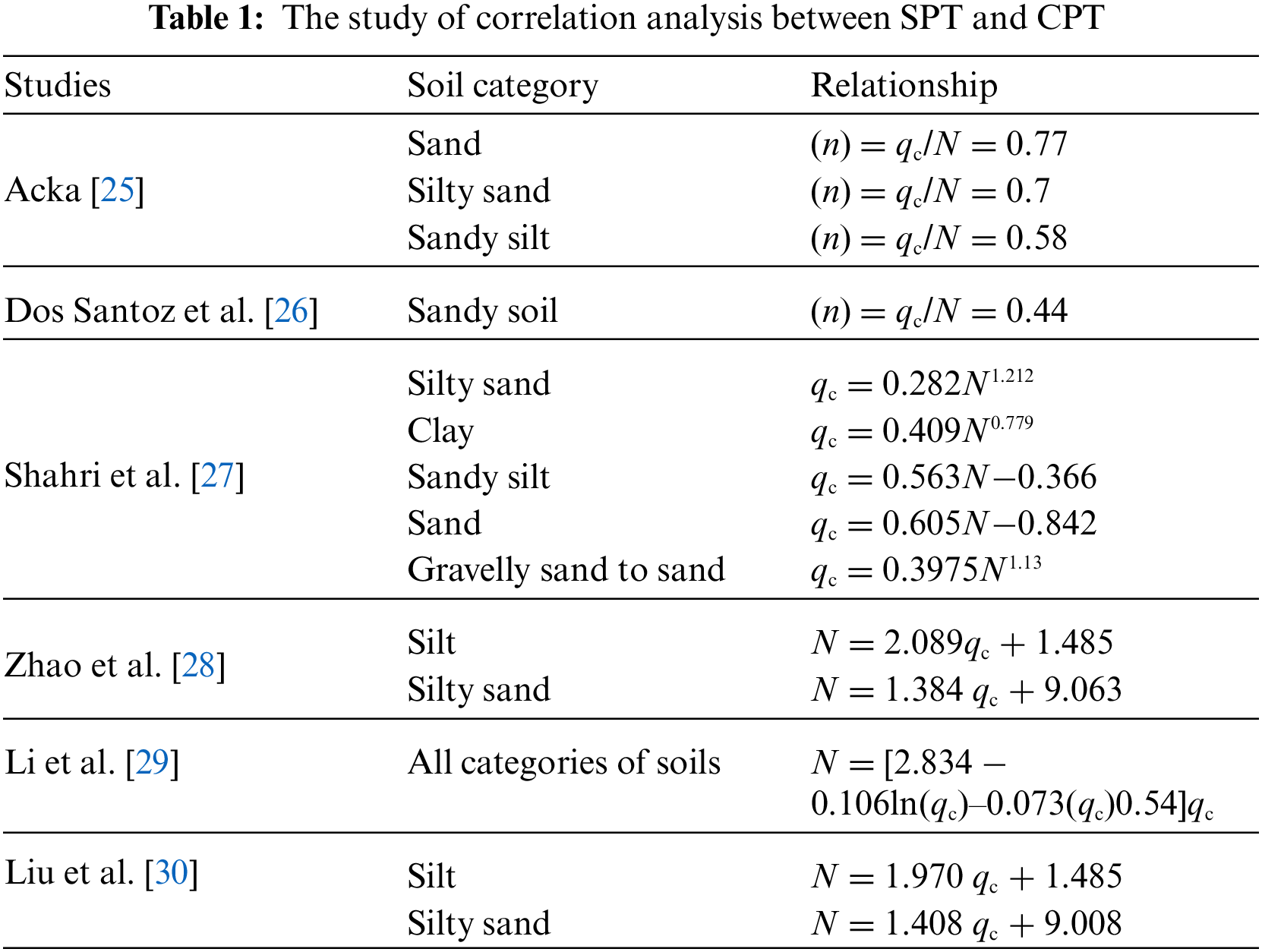
Table 1 lists studies about empirical equations for predicting N based on one or more CPT parameters, and these methods mainly use regression analysis to establish the relationship. Acka [25] investigated the correlation between SPT and CPT data in the UAE and proposed an empirical equation to predict CPT values from SPT data. Dos Santoz et al. [26] developed correlation models between SPT-CPT and DPL-CPT data for sandy soils in Brazil. Shahri et al. [27] performed statistical analysis to develop a high-accuracy correlation model between SPT and CPT data. Zhao et al. [28] established correlations between SPT and CPT parameters for liquefaction evaluation in China, proposing two correlation equations for N value and qc. Li et al. [29] used the least squares method to establish a regression model between N with qc and investigated the impact of three factors on liquefaction discrimination. Liu et al. [30] determined the selection principle of SPT-CPT comparison holes and the acquisition method of parameters in several actual projects, and further used statistical methods to fit the scatter plot formed by N and qc values. The emergence of artificial intelligence has given rise to the widespread use of intelligent techniques for problem-solving in science and engineering. Among these techniques, machine learning has proven to be a powerful tool for extracting information from data. Recently, it has been increasingly applied to predict the N value using CPT parameters. Tarawneh [31] analyzed a dataset consisting of both SPT and CPT data and used the Artificial Neural Networks (ANN) model to predict the N value from the CPT data. The study found that the ANN model provided accurate predictions of the N value, demonstrating the potential for using this approach as an alternative to traditional SPT testing. Fernando et al. [32] explored the feasibility of using ANN to predict SPT values and compared the prediction accuracy with and without data normalization. The study found that an ANN model using CPT data and soil properties as input variables could accurately predict SPT values, with data normalization further improving the accuracy and reliability of the predictions. Gupta et al. [33] investigated the correlations between SPT and CPT data for liquefaction assessment using the statistical programming language R. The study compared different correlation methods and found that the developed correlations using the random forest regression method provided the best prediction accuracy.

To match CPT and SPT data, many of the above studies have employed the method of averaging CPT parameters or selecting representative values within a given soil layer to correspond to N values. This method has the advantage of being simple and easy to implement. However, it is important to note that this approach has some limitations. One limitation is that this method may overlook critical local or inhomogeneous features. Averaging or selecting representative values may smooth out small-scale variations within the soil layer, and these variations may be important for understanding the geotechnical behavior of the soil. Another potential limitation of averaging or selecting representative values for CPT data is that it may obscure the variability between different categories of soil layers. Soil layers can exhibit different geotechnical properties, and ignoring this variability can lead to inaccurate correlations between the CPT and SPT data. When performing CPT and SPT data matching, factors such as soil properties, structure, and variability characteristics usually need to be considered to obtain accurate and reliable matching results.

To address a common problem faced by current SPT-CPT correlation studies, this study proposed to correspond to N values by establishing the CPT feature matrix. The CPT feature matrix consists of the CPT parameters of the two CPT exploration holes closest to the SPT exploration holes within a given soil layer. The numerical matrix divides the CPT data of different exploration holes into different column vectors. By doing so, the CPT feature matrix approach can make full use of the information from multiple exploration holes, allowing for the extraction of richer information regarding soil characteristics. Additionally, the numerical matrix approach divides the CPT data into different row vectors based on the different depths of CPT parameters. This method enables the extraction of feature information at different depths, which accurately reflects the changing characteristics of soil properties. In contrast, the averaging method simply averages the CPT data, which may not fully capture the local variations in depth and can lead to inaccuracies in characteristic soil estimations. Drawing inspiration from the characteristics of Convolutional Neural Network (CNN) in image recognition [34,35], the paperproposed that a sliding window function performing the convolution principle can be effectively applied to the constructed CPT feature matrix. As the convolution kernel slides over the matrix, the features are integrated by multiplying the convolution kernel with the input matrix. The CNN network performs higher-level feature extraction on the input CPT feature matrix to predict the N value.

In summary, this paper presents a novel approach for establishing the correlation between N and CPT parameters using the CNN model. The Genetic Algorithm (GA) is utilized to optimize the CNN network hyperparameters in a data-driven manner. The model can predict the values of N based on the CPT parameters. Finally, the predicted N values are expected to be used for assessing the liquefaction potential based on the discriminatory liquefaction method outlined in the Chinese Specification for Seismic Design of Buildings.

The remainder of this paper is as follows: Section 2 introduces the experimental data used in this paper and data pre-processing work; Section 3 introduces the principle of CNN and GA; Section 4 presents the establishment of the optimized CNN model; Section 5 shows a comparative study with the empirical methods; Section 6 demonstrates the feasibility of utilizing the predicted N values obtained from proposed model for liquefaction discrimination.

2  Experimental Data Introduction

2.1 Data Source

The standard penetration test blow count N is a crucial geotechnical parameter that reflects soil resistance properties. It is determined by counting the number of blows required to drive a split-spoon sampler 30 cm into the soil using standard energy of 60 joules per blow during the SPT (Fig. 1a). The tip resistance qc and sleeve resistance fs, obtained through the CPT, are equally important geotechnical parameters for evaluating soil mechanical properties. The qc value measures the resistance of a cone-shaped penetrometer to penetration into the soil at a constant rate, while the fs value measures the resistance of the penetrometer’s side friction against the soil (Fig. 1b).

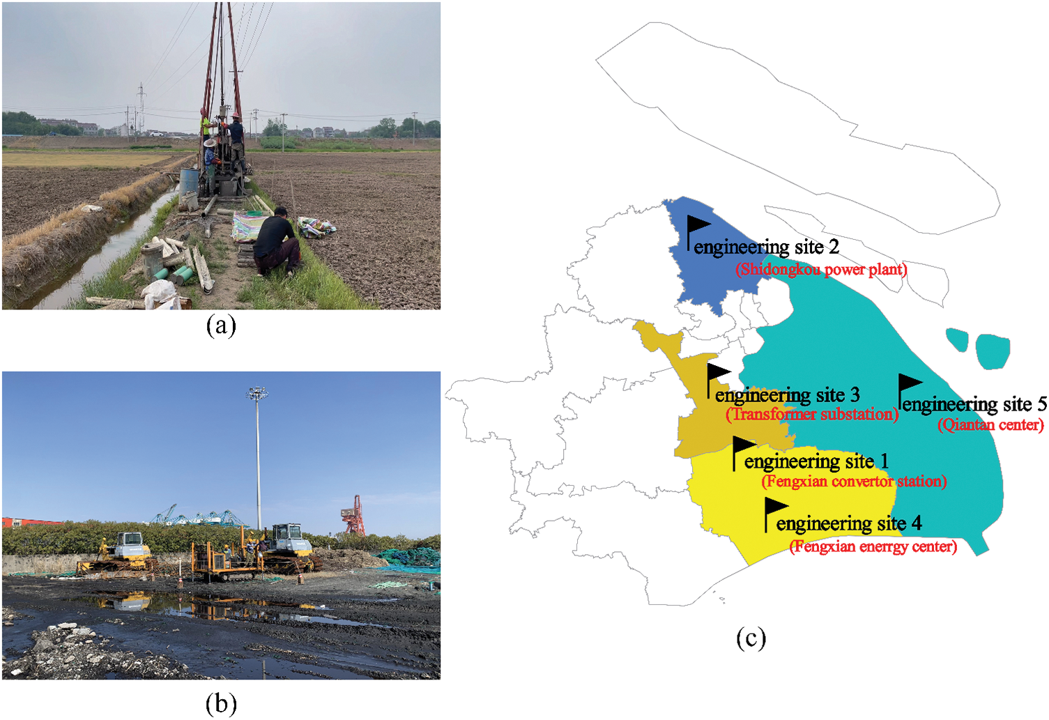
Figure 1: Data source: (a) Standard penetration test; (b) Cone penetration test (c) The location of the engineering site

The experimental data were collected from five investigation engineering sites in Shanghai, China, as shown in Fig. 1c. The whole data included 138 SPT exploration holes and 198 CPT exploration holes, with the number of exploration holes varying across each site. Specifically, the number of exploration holes for each site is statistically illustrated as follows:

Engineering site 1: 25 SPT exploration holes and 41 CPT exploration holes

Engineering site 2: 42 SPT exploration holes and 63 CPT exploration holes

Engineering site 3: 7 SPT exploration holes and 14 CPT exploration holes

Engineering site 4: 20 SPT exploration holes and 27 CPT exploration holes

Engineering site 5: 44 SPT exploration holes and 53 CPT exploration holes

2.2 Abnormal Data Filtering

This research investigates three categories of soil layers: sandy silt, silty sand, and clayey silt. To ensure that the data used for correlation analysis is of good quality and reduces the risk of overfitting during model training, the box plot method [36] is used to identify and remove outliers from the experimental dataset. It works by first arranging the data in ascending order and then calculating statistical metrics such as the median value, quartiles Q1 and Q3, and the interquartile range (IQR). The upper limit (UL) and lower limit (LL) are then calculated based on the quartiles and IQR. Data points outside the UL and LL are considered outliers and removed from the dataset. Figs. 2–4 illustrate the distribution of both raw and filtered data for different soil categories, including sandy silt, silty sand, and clayey silt. The removal of data outliers leads to a more concentrated data distribution, significantly reducing the impact of outliers on data analysis and improving the reliability of data analysis.

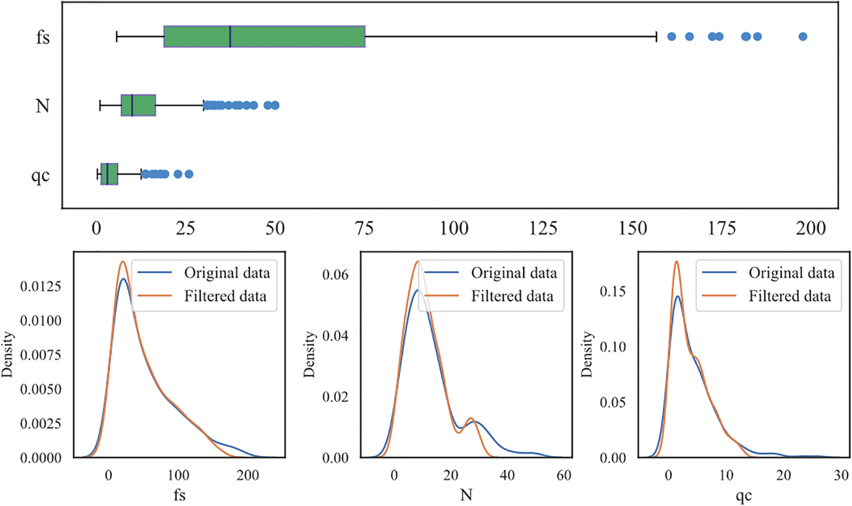
Figure 2: Abnormal data filtering (sandy silt)

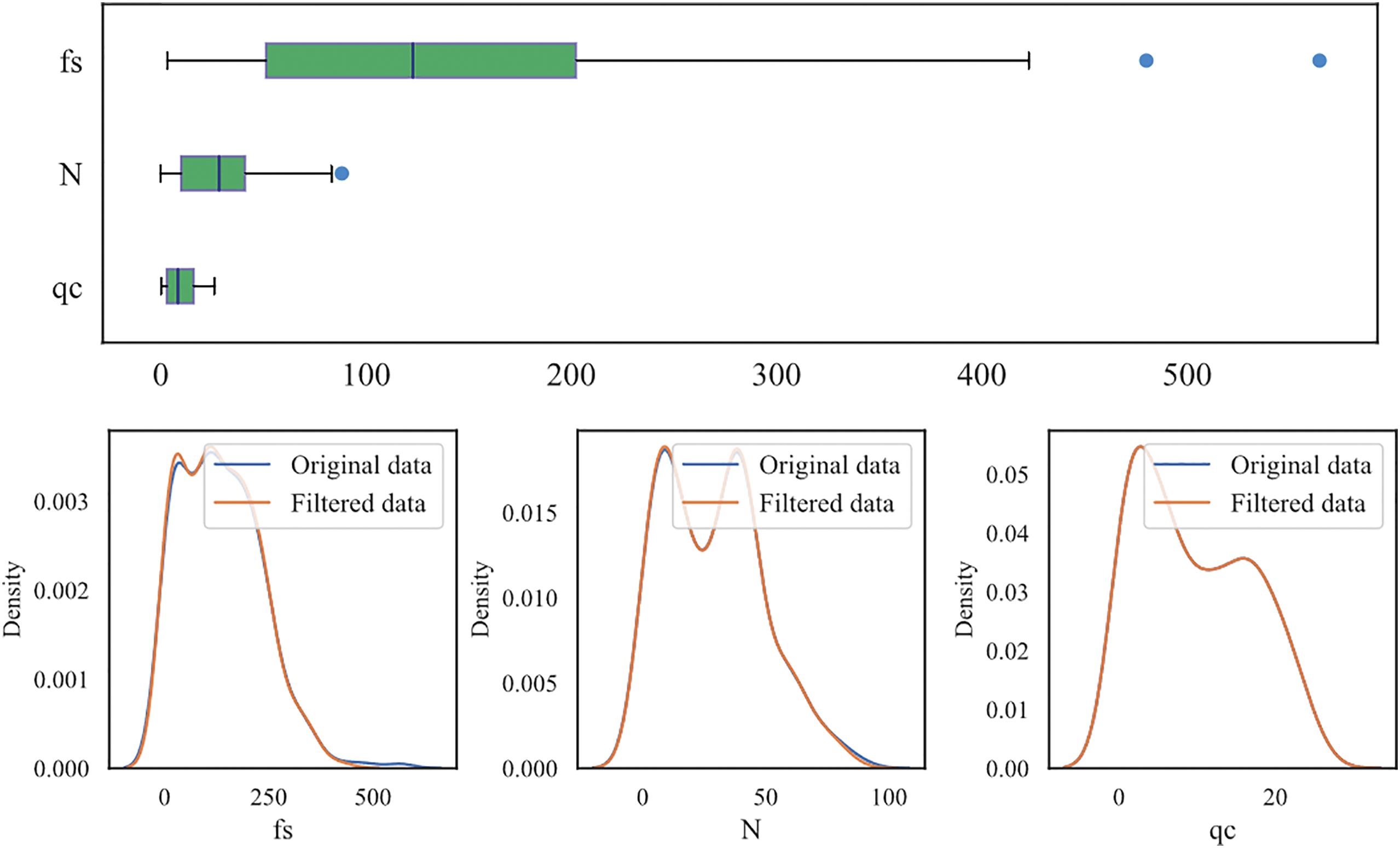
Figure 3: Abnormal data filtering (silty sand)

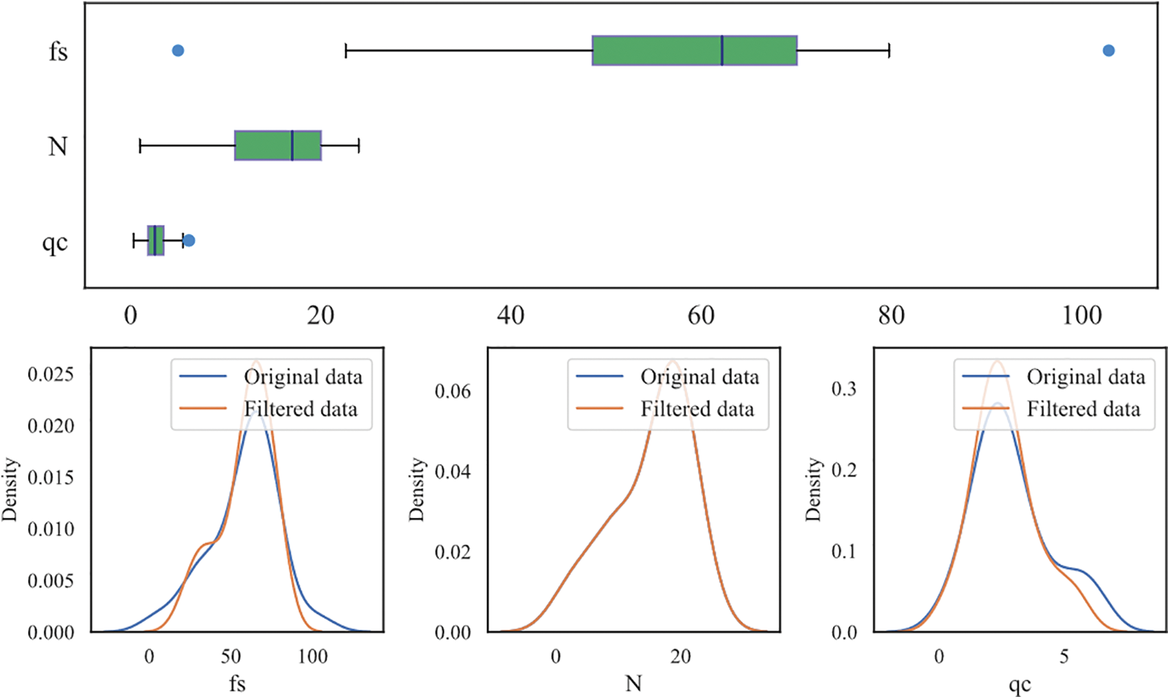
Figure 4: Abnormal data filtering (clayey silt)

2.3 The Matching Principle between CPT and SPT Data

The data of SPT is discrete, while the data of CPT is continuous, and a principle needs to be established to match the SPT and CPT data. This study proposes a solution using the CPT feature matrix to match the N value. First, the maximum distance between CPT and SPT was set at 30 m, and only data within this range was considered for correlation analysis. In the vertical direction, the upper and lower 0.2 m of each depth of the N value were taken as the soil’s upper and lower characteristic boundary to capture the detailed variance characteristics of CPT data. For the horizontal direction, the CPT hole with the two closest distances to the SPT exploration hole was selected. The feature matrix corresponding to the N was established based on the qc, fs, and H of the two selected CPT holes (Fig. 5). Note that SPT exploration holes without a nearby CPT hole within 30 m were eliminated. If only one CPT hole was available, its feature information was duplicated to establish the feature matrix.

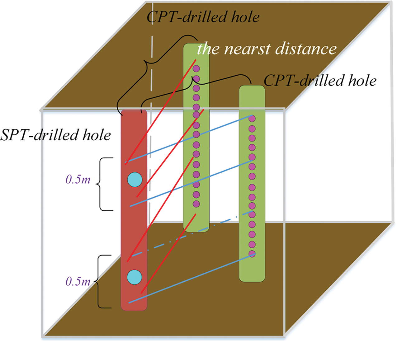
Figure 5: The matching principle between SPT and CPT

As described in Eq. (1), the CPT feature matrix consists of the CPT parameters of the two CPT exploration holes closest to the SPT exploration holes within a given soil layer.

X=(x(1),H,x(2))=|qc(1)fs(1)Hi+0.2fs(2)qc(2)qc(1)fs(1)Hi+0.1fs(2)qc(2)qc(1)fs(1)Hifs(2)qc(2)qc(1)fs(1)Hi−0.1fs(2)qc(2)qc(1)fs(1)Hi−0.2fs(2)qc(2)|5×5(1)

where X refers to the CPT characteristic matrix corresponding to N, x refers to the CPT hole with the two closest distances to the SPT hole, i refers to the penetration depth of SPT, and the subscripts (1) and (2) at the top right corner of x refer to the number of CPT exploration hole that is closest to the SPT exploration hole, respectively.

The proposed method utilizes a CNN model to establish the relationship between the CPT feature matrix and N. Through the sliding window function, the convolution kernel integrates the qc and fs information from different depths of the first CPT exploration hole (Fig. 6a), then integrates the fs information and depth H (Fig. 6b). Subsequently, the window integrates CPT information from the second exploration hole (Figs. 6c and 6d). When the window slides down to the next level, it can integrate CPT information from different depths (Fig. 6e).

Figure 6: The principle of feature fusion based on the feature matrix

3  Analytical Method

3.1 Machine Learning Algorithm CNN

CNN is a powerful machine learning algorithm that uses convolutional operations for feature extraction and a layered combination of neural networks to learn complex data efficiently. The convolution operation refers to sliding a data window to different locations of the input data, then performing dot product and accumulation operations on the data in the window with a convolution kernel (also called a filter) to obtain the output feature map, as shown in Eq. (2):

aij=f(∑m=02∑n=02ωm,nxi+m,j+n+ωb)(2)

where xij refers to the value of the ith row and jth column of the input matrix, aij refers to the value of the ith row and jth column of the output matrix, f refers to the activation function, wm,n refers to the weight assigned by the filter to the mth row and nth column of the input matrix, wb refers to the bias assigned by the filter.

CNN consists of multiple convolutional, pooling, activation functions, and fully connected layers (Fig. 7). The input values are passed through the layers to the final output layer. Eq. (3) is the formula for calculating the difference between the output and the true values.

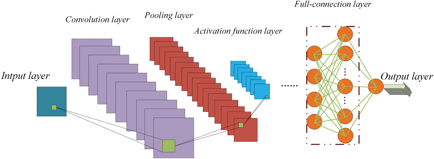
Figure 7: CNN algorithm

J=12(yfianl−ytrue)2(3)

During the training process, CNN improves the accuracy and generalization of the model by continuously adjusting the parameters of the convolutional kernel and the weights between neurons, as described in Eqs. (4) and (5):

(W,b)=arg⁡min(J(w,b))(4)

(W,b)n+1=(W,b)n−r⋅grad(J(W,b)n)(5)

where r refers to the learning rate, and grad refers to the derivative of the loss function J to the w or b.

3.2 Genetic Algorithm

The Genetic Algorithm (GA) is a powerful optimization algorithm that simulates the process of natural selection and biological evolution in nature. As shown in Fig. 8, the GA converts multiple problem solutions into corresponding chromosomes, which are then evaluated based on their fitness to the problem. The chromosomes with higher fitness are selected and undergo genetic operations, including gene exchange and mutation. The process of selection, elimination, mutation, and exchange is repeated multiple times until the remaining chromosomal genes represent the most optimal solution to the problem.

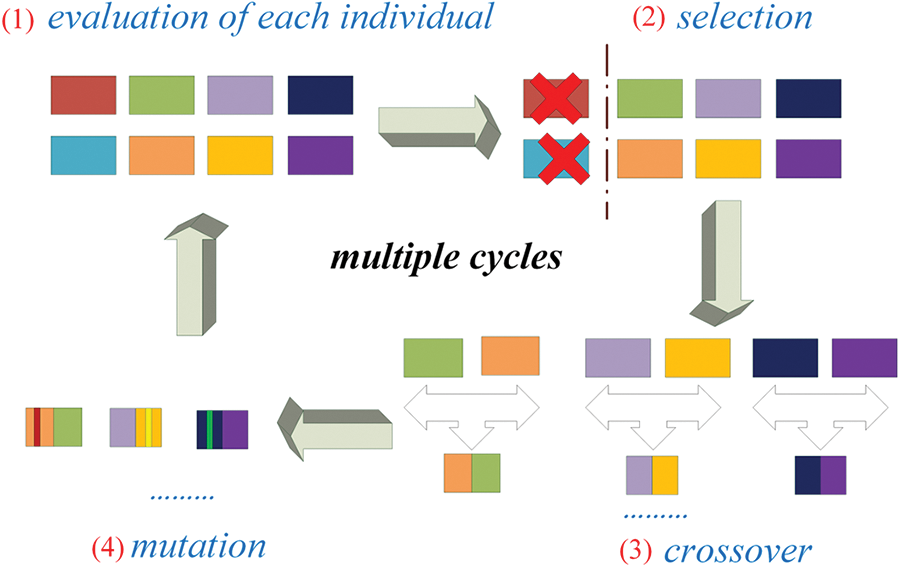
Figure 8: Genetic algorithm

3.3 Evaluation Metric

Mean absolute error (MAE), root mean square error (RMSE), mean squared error (MSE), and the coefficient of determination R2 are the metrics used to evaluate the model performance in this paper. MAE represents the average of the absolute error, which can better reflect the actual situation of the prediction value error. RMSE is a measure of the dispersion of the sample distribution, indicating the deviation between the observed value and the true value, and is often used as a standard for measuring the prediction results of machine learning models. MSE is a more common error calculation in statistics, which is the expectation of the error square between the true value and the predicted value. R2 is a metric used to evaluate regression models, which indicates the proportion of the variance in the data that the model can explain. Generally, the closer to 1, the smaller the error between the predicted and true values. The above metrics are calculated by:

MAE=1N∑i=1N|yi∧−yi|(6)

RMSE=1N∑i=1N(yi∧−yi)2(7)

MSE=1N∑i=1N(yi∧−yi)2(8)

R2=1−∑i=1N(yi∧−yi)2∑i=1N(yi−yi−)2(9)

where yi is the true value, y^i is the predicted value, y¯i is the average value of the true values, and N is the number of data.

To certify the robustness of the model, the cross-validation method was introduced in this study. The method evenly divides the whole data into several groups, selecting one as the testing dataset, while the corresponding remaining part is the training dataset. Each data group was selected as the testing dataset and avoided overlapping with the data from the training dataset. Take the average of all testing dataset scores as the final model performance score, which is calculated in Eq. (10):

CV(k)=1k∑i=1kRi2(10)

where k refers to the number of groups of all datasets that were divided, and R2i refers to the R2 value when the ith group dataset is the testing dataset.

4  The Optimization of the CNN Model

The structure of the CNN model, especially the number of filters per convolutional layer and neurons per full-connection layer, significantly impacts the model performance. Therefore, optimizing the model structure is crucial to achieving high accuracy and efficiency. In this study, the genetic algorithm was utilized to optimize the structure of the model. The designed CNN network comprises five layers, including three convolutional layers and two fully connected layers. The structural information of the model was encoded as chromosomes, as presented in Fig. 9.

Figure 9: The optimization of the CNN model structure

Each chromosome consists of five parameters, with the first three determining the number of filters per convolutional layer, ranging from 1 to 20, and the last two determining the number of neurons per fully connected layer, ranging from 1 to 15. The fitness of each chromosome was calculated using Eq. (11), where chromosomes with higher fitness correspond to superior model structures and are thus more likely to be inherited to the next generation. The probability of inheritance for each chromosome was determined using Eq. (12), which calculates the ratio of the fitness of that chromosome to the sum of the fitness values of the entire population. The chromosomes with greater fitness have a higher probability of being selected and could potentially be selected multiple times, further improving the average performance of the next-generation model. The hyperparameters of the genetic algorithm are summarised in Table 2. For more information, refer to Appendix A for the pseudocode of optimizing the CNN model using the genetic algorithm.

fitnessi=CV(10,R2)(populationi)=CV(10,R2)(Modeli(a,b))(11)

probabilityi=fitnessi∑k=1Kfitnessk(12)

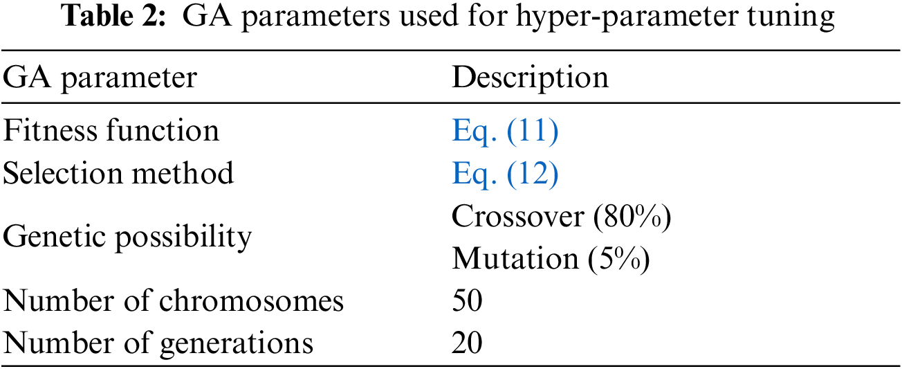
where i refers to each population, K refers to the number of populations, and a, b refers to the number of filters per convolutional layer and the number of neurons per full connection layer.

The optimal combination of filter and neuron numbers for the model could be identified by using the GA algorithm for tuning the hyperparameters of the CNN model. Fig. 10 illustrates the convergence of the average population fitness after several generations of selection, exchange, and mutation, indicating the effectiveness of the Genetic Algorithm in hyperparameter tuning. In our study, the optimized model had three convolutional layers with 9, 7, and 13 filters, respectively, and two full-connection layers with 12 and 8 neurons. The use of the Genetic Algorithm greatly reduced the workload of the optimization process compared to permutation or variable analysis, which is time-consuming and inefficient.

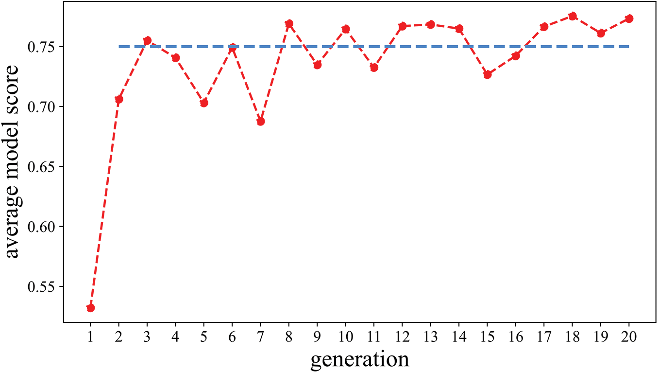
Figure 10: Average value of model score vs. generation

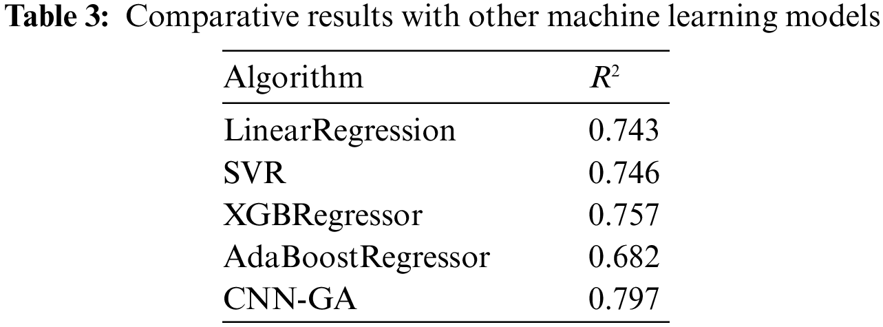
Table 3 compares the performance of the optimized CNN model with other machine-learning algorithms. The results indicate that the optimized CNN model outperforms the other models with a minimum error, demonstrating that it is the most suitable model for this particular scenario. The R2 values obtained for the optimized CNN model (0.797) are higher than those obtained for the other models, including Linear Regression (0.743), SVR (0.746), XGBRegressor (0.757), and AdaBoostRegressor (0.682). Furthermore, the feature matrix computation based on the convolution principle is interpretable in fusing multifaceted features, which enhances the researchers’ comprehension of the model. Therefore, the optimized CNN model is a promising approach for predicting the outcome of this specific task.

5  Analysis of the Built Model

5.1 Comparison with the Equation Methods

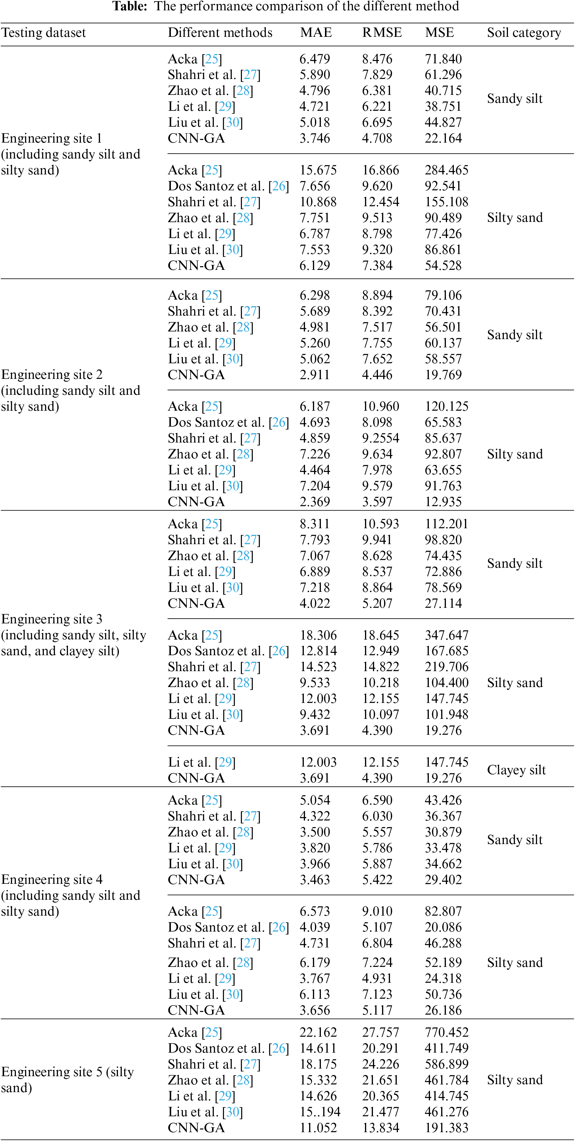
This section compares the prediction of the CNN-GA model with equation methods in terms of N values for various soil categories. The characteristics of datasets from the same engineering site are likely to be similar. Therefore, a model trained on data from one engineering site may perform well when tested on data from the same site, but it may not perform as well when tested on data from a different site. To ensure the robustness and generalizability of the models across different sites, the training and testing datasets were divided based on engineering sites. A cross-validation approach was utilized, where the test set consisted of data from one engineering site while the training set comprised data from the other engineering sites. This approach ensured that the models were trained and tested on a diverse set of data, enabling them to be more robust and generalizable. This method provides a stringent test of the generalizability of our model, as it ensures that there is no overlap or similarity between the data in the training and testing sets.

This section only analyzes the performance of the models when data from engineering site 1 is used as the testing set and the data from the remaining engineering sites are used as the training set, and other cases are detailed in Appendix B. The soil at engineering site 1 contains two main categories, including sandy silt and silty sand, and this section analyzes them separately. The comparison results are presented through scatter distribution and frequency distribution graphs. The scatter distribution graph shows the true and predicted values on the horizontal and vertical axes, respectively. Points closer to the diagonal indicate a smaller discrepancy between the predicted and true values. In a frequency distribution plot, the ratio of predicted to true values for a given sample is represented by the variable n. The frequency distribution curve of n is more centralized at x = 1 means the prediction result is accurate.

For sandy silt (Fig. 11), Acka [25] and Shahri et al. [27] consistently underestimated true N values, and Zhao et al. [28], Li et al. [29], and Liu et al. [30] performed poorly for data with true values above 30. In contrast, the CNN-GA model provided more accurate predictions, especially for data with smaller true values.

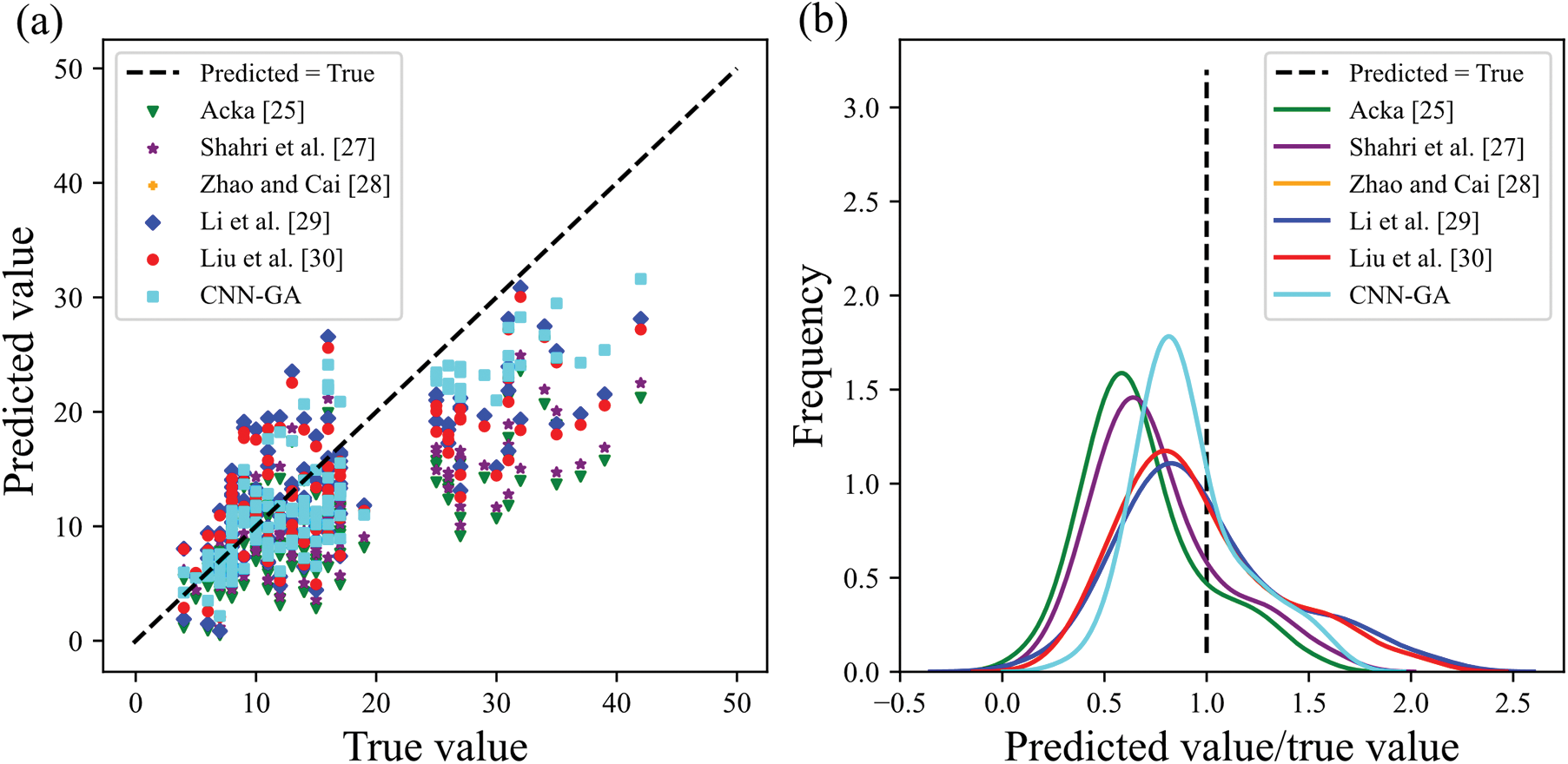
Figure 11: The comparative prediction results of different methods for N (sandy silt)

Compared to the CNN-GA model, the traditional methods of Acka [25], Dos Santoz et al. [26], Shahri et al. [27], Zhao et al. [28], Li et al. [29], and Liu et al. [30] for predicting N values in silty sand yielded poor results (Fig. 12). Specifically, Acka [25], Dos Santoz et al. [26], and Shahri et al. [27] produced predicted values that were significantly far from the true N values; Zhao et al. [28], Li et al. [29], and Liu et al. [30] consistently underestimated the true N values. In contrast, the CNN-GA model demonstrated superior predictive performance for silty sand, outperforming traditional methods in terms of accuracy.

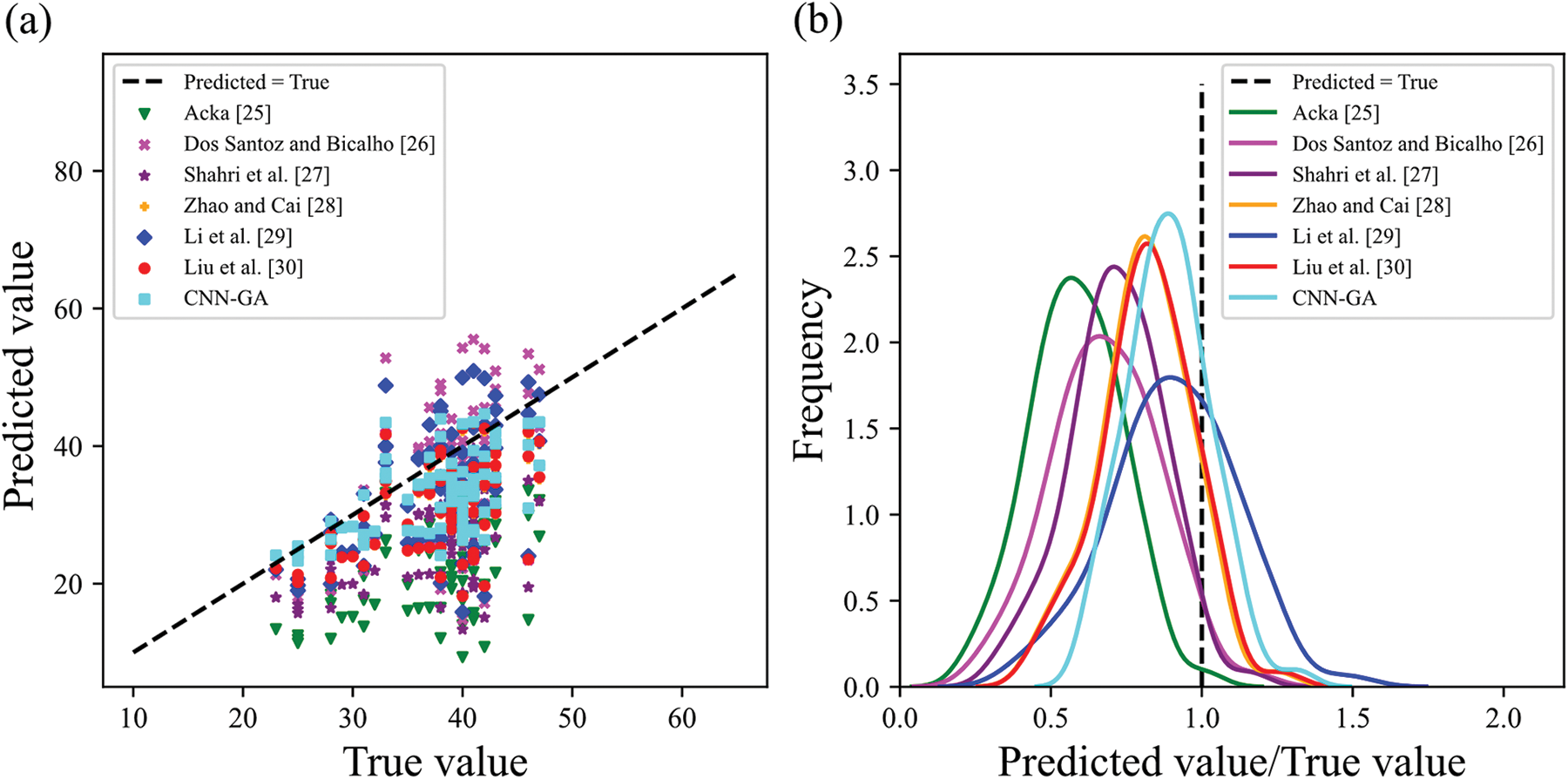
Figure 12: The comparative prediction results of different methods for N (silty sand)

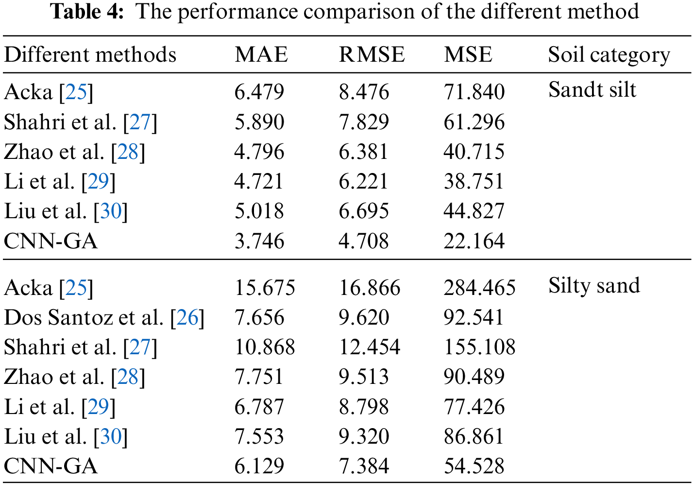
Table 4 presents the error metrics of various models for different soil categories, including sandy silt, silty sand, and clayey silt. The results demonstrate that the CNN-GA model studied in this paper outperformed other studies, achieving lower MAE, RMSE, and MSE values for all three soil categories. In addition to the improved accuracy, the CNN-GA model is a comprehensive model that predicts soil parameters without prior knowledge of soil category, which makes it an attractive alternative to other methods.

5.2 The Analysis of CNN-GA Model Prediction Results

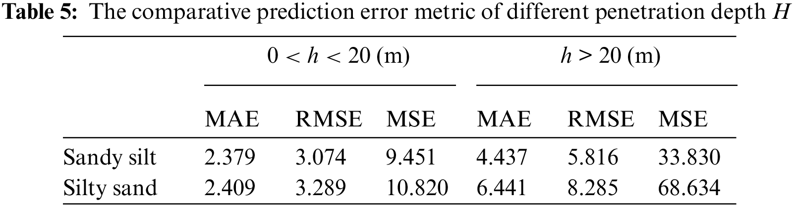
This section further analyzed the prediction accuracy of our proposed model for N values at different soil depths. Fig. 13 illustrates the discrepancy between the predicted and true values of N, and the prediction results for relatively deep soil layers are not well. However, the liquefaction discrimination problem focuses primarily on soils within 20 m below ground, so the poor predicted results for deep soils have less impact on the latter study of liquefaction discrimination. Table 5 summarizes the error metrics of different categories of soils in different depth ranges. The result showed that the prediction for the soil with a depth of less than 20 m has a minor error, which is more beneficial to the subsequent liquefaction discrimination study. The results demonstrate that the model has minor prediction errors for soils with a depth of less than 20 m, which is particularly beneficial for subsequent liquefaction discrimination studies.

Figure 13: Analysis of CNN-GA model prediction results

6  The Application of Liquefaction Discrimination Based on the Built Model

This section demonstrates the feasibility of utilizing the predicted N values for liquefaction discrimination. The approach for liquefaction discrimination utilized in this study was based on the code for the seismic design of buildings (GB50011-2010). According to this code, liquefaction is considered to occur when the standard penetration test blow count N of the saturated soil is less than or equal to the critical value Ncr. The formula for Ncr is given in Eq. (13):

Ncr=N0β[ln⁡(0.6ds+1.5)−0.1dw]3/ρc(13)

where N0 is the reference value of the SPT for liquidation discrimination, ds is the penetration depth (m), dw is the depth of the groundwater level (m), ρc is the percentage of clay, and β is the regulation factor.

After determining the Ncr value based on soil factors, the predicted and measured N values were compared with Ncr for each exploration hole to assess the liquefaction potential. Take engineering site 1 as an illustration, and the liquefaction discrimination results are summarized in Table 6. The number 0 in the table indicates that the sample is classified as liquefied, while the number 1 indicates that the sample is classified as non-liquefied. √ represents consistent discriminatory results, while × represents inconsistent discriminatory results. The results showed that the discriminatory results based on predicted N values had a consistency of 75% with the results obtained from measured N values, indicating the reliability of the proposed model in evaluating the liquefaction potential of an engineering site. Moreover, using predicted N values can significantly reduce the workload and time required for geotechnical personnel to perform liquefaction assessments, particularly when many SPT exploration holes need to be tested. At the initial stage of liquefaction discrimination, a preliminary assessment can be conducted using the predicted N values, and the SPT can be selectively performed based on the preliminary results for further evaluation. This simplified and efficient approach can enhance the effectiveness of the geotechnical investigation, making our proposed model a valuable tool for geotechnical engineers.

7  Conclusion

The CPT feature matrix is a novel feature extraction method proposed in this study, which converts the traditional CPT test data into a matrix form for processing. Each element in the feature matrix represents the CPT data at a specific depth, such as tip resistance qc and sleeve resistance fs. By convolving the feature matrix, the multidimensional features were fused, effectively improving the prediction accuracy of the N value. Additionally, the Genetic Algorithm (GA) was employed to optimize the model and improve its accuracy and generalization. The study verified the prediction performance of the model for different soil categories, and the results showed that the method has higher prediction accuracy than the conventional method. Then the study validates the feasibility of liquefaction discrimination based on the developed model. The study utilized the predicted N values obtained from the model for liquefaction discrimination and compared the results with the measured N values, using the liquefaction discrimination criteria outlined in the seismic design code for buildings (GB50011-2010). The experimental results show that the agreement between the liquefaction discrimination results based on the predicted N values and the measured N values is 75%, which indicates that the proposed model has reliability in assessing the liquefaction potential of the engineering site.

Given the high level of uncertainty associated with geotechnical engineering, the feature matrix proposed in this study has the potential for broad applications in other geoengineering fields. The use of multidimensional features can improve the accuracy and reliability of predictions in contexts where data is often limited and uncertainty is high. Although this study yielded some meaningful results, some shortcomings need to be acknowledged. The primary deficiencies of this study include:

1. While the proposed method has shown promising results for liquefaction discrimination, its reliability needs to be further verified in multiple regions. There is also scope for refinement and enhancement of the method in the future. To this end, we intend to conduct further studies and collect data on liquefaction cases in China to verify the effectiveness of our proposed method.

2. The current study did not include a comparison with other state-of-the-art AI methods, such as related deep learning methods, because it would involve the authors’ source code and experimental data. In future studies, we plan to include more comprehensive and systematic comparisons with other methods to provide a more thorough understanding of the effectiveness of our proposed method.

Acknowledgement: The authors thank the reviewers who remained anonymous for their constructive criticism and recommendations, which helped to make the manuscript better.

Funding Statement: This study was supported by the Center University (Grant No. B220202013) and Qinglan Project of Jiangsu Province (2022).

Author Contributions: Ruihan Bai wrote the main manuscript text and performed the experiments. Feng Shen gave guidance and suggestions for method of this article, as well as reviewed and edited the manuscript. Zihao Zhao summarized the methods of the existing related research. Zhiping Zhang drew the diagrams (model structure in the article and provided suggestions for improving the article's layout. Qisi Yu contributed to the check, review, and editing of the article. All authors reviewed and revised the manuscript.

Availability of Data and Materials: The data supporting the conclusions of this article are included within the article. Any queries regarding these data may be directed to the author Ruihan Bai (bairuihanup@163.com).

Conflicts of Interest: The authors declare that they have no conflicts of interest to report regarding the present study.

References

1. Seed, H. B., Idriss, I. M. (1967). Analysis of soil liquefaction: Niigata earthquake. Journal of the Soil Mechanics and Foundations Division, 93(3), 83–108. [Google Scholar]

2. Huang, Y., Yu, M. (2013). Review of soil liquefaction characteristics during major earthquakes of the twenty-first century. Natural Hazards, 65, 2375–2384. [Google Scholar]

3. Singh, S. (1996). Liquefaction characteristics of silts. Geotechnical & Geological Engineering, 14, 1–19. [Google Scholar]

4. Shu, S., Ge, B., Wu, Y., Zhang, F. (2023). Probabilistic assessment on 3D stability and failure mechanism of undrained slopes based on the kinematic approach of limit analysis. International Journal of Geomechanics, 23(1), 06022037. [Google Scholar]

5. Shibata, T., Oka, F., Ozawa, Y. (1996). Characteristics of ground deformation due to liquefaction. Soils and Foundations, 36, 65–79. [Google Scholar]

6. Goda, K., Atkinson, G. M., Hunter, J. A., Crow, H., Motazedian, D. (2011). Probabilistic liquefaction hazard analysis for four Canadian cities. Bulletin of the Seismological Society of America, 101(1), 190–201. [Google Scholar]

7. Subedi, M., Acharya, I. P. (2022). Liquefaction hazard assessment and ground failure probability analysis in the Kathmandu Valley of Nepal. Geoenvironmental Disasters, 9(1), 1–17. [Google Scholar]

8. Piya, B., van Westen, C., Woldai, T. (2004). Geological database for liquefaction hazard analysis in the Kathmandu Valley, Nepal. Journal of Nepal Geological Society, 30, 141–152. [Google Scholar]

9. Putti, S. P., Satyam, N. (2018). Ground response analysis and liquefaction hazard assessment for Vishakhapatnam City. Innovative Infrastructure Solutions, 3, 1–14. [Google Scholar]

10. Ansari, A., Zahoor, F., Rao, K. S., Jain, A. K. (2022). Liquefaction hazard assessment in a seismically active region of Himalayas using geotechnical and geophysical investigations: A case study of the Jammu Region. Bulletin of Engineering Geology and the Environment, 81(9), 349. [Google Scholar]

11. Seed, H. B., Idriss, I. M. (1971). Simplified procedure for evaluating soil liquefaction potential. Journal of the Soil Mechanics and Foundations Division, 97(9), 1249–1273. [Google Scholar]

12. Cetin, K. O., Seed, R. B., Kayen, R. E., Moss, R. E., Bilge, H. T. et al. (2018). Examination of differences between three SPT-based seismic soil liquefaction triggering relationships. Soil Dynamics and Earthquake Engineering, 113, 75–86. [Google Scholar]

13. Robertson, P. K., Campanella, R. G. (1985). Liquefaction potential of sands using the CPT. Journal of Geotechnical Engineering, 111(3), 384–403. [Google Scholar]

14. Robertson, P. K., Wride, C. E. (1998). Evaluating cyclic liquefaction potential using the cone penetration test. Canadian Geotechnical Journal, 35(3), 442–459. [Google Scholar]

15. Juang, C. H., Chen, C. J., Jiang, T., Andrus, R. D. (2000). Risk-based liquefaction potential evaluation using standard penetration tests. Canadian Geotechnical Journal, 37(6), 1195–1208. [Google Scholar]

16. Missoum, H., Belkhatir, M., Bendani, K., Maliki, M. (2013). Laboratory investigation into the effects of silty fines on liquefaction susceptibility of Chlef (Algeria) sandy soils. Geotechnical and Geological Engineering, 31, 279–296. [Google Scholar]

17. Liu, J. (2020). Influence of fines contents on soil liquefaction resistance in cyclic triaxial test. Geotechnical and Geological Engineering, 38(5), 4735–4751. [Google Scholar]

18. Zhao, Z., Duan, W., Cai, G., Wu, M., Liu, S. (2022). CPT-based fully probabilistic seismic liquefaction potential assessment to reduce uncertainty: Integrating XGBoost algorithm with Bayesian theorem. Computers and Geotechnics, 149, 104868. [Google Scholar]

19. Zhao, Z., Duan, W., Cai, G. (2021). A novel PSO-KELM based soil liquefaction potential evaluation system using CPT and Vs measurements. Soil Dynamics and Earthquake Engineering, 150, 106930. [Google Scholar]

20. Fang, Y., Jairi, I., Pirhadi, N. (2023). Neural transfer learning for soil liquefaction tests. Computers & Geosciences, 171, 105282. [Google Scholar]

21. Zhang, Y., Xie, Y., Zhang, Y., Qiu, J., Wu, S. (2021). The adoption of deep neural network (DNN) to the prediction of soil liquefaction based on shear wave velocity. Bulletin of Engineering Geology and the Environment, 80, 5053–5060. [Google Scholar]

22. Bray, J. D., Sancio, R. B. (2006). Assessment of the liquefaction susceptibility of fine-grained soils. Journal of Geotechnical and Geoenvironmental Engineering, 132(9), 1165–1177. [Google Scholar]

23. Shengcong, F., Tatsuoka, F. (1984). Soil liquefaction during Haicheng and Tangshan earthquake in China; A review. Soils and Foundations, 24(4), 11–29. [Google Scholar]

24. Huang, Y., Jiang, X. (2010). Field-observed phenomena of seismic liquefaction and subsidence during the 2008 Wenchuan earthquake in China. Natural Hazards, 54, 839–850. [Google Scholar]

25. Akca, N. (2003). Correlation of SPT-CPT data from the United Arab Emirates. Engineering Geology, 67(3–4), 219–231. [Google Scholar]

26. Dos Santos, M. D., Bicalho, K. V. (2017). Proposals of SPT-CPT and DPL-CPT correlations for sandy soils in Brazil. Journal of Rock Mechanics and Geotechnical Engineering, 9(6), 1152–1158. [Google Scholar]

27. Shahri, A., Juhlin, C., Malemir, A. (2014). A reliable correlation of SPT-CPT data for Southwest of Sweden. Electronic Journal of Geotechnical Engineering, 19, 1013–1032. [Google Scholar]

28. Zhao, X., Cai, G. (2015). SPT-CPT correlation and its application for liquefaction evaluation in China. Marine Georesources & Geotechnology, 33(3), 272–281. [Google Scholar]

29. Li, G., Guo, W., Qiao, L. (2018). Study on the method of site liquefaction discrimination based on CPT in Jiangsu area. Site Investigation Science and Technology, 221(1), 10–13. [Google Scholar]

30. Liu, X., Huang, Z., Ren, Y., Chen, N. (2012). The analysis of SPT-CPT correlation and influencing factors. Science Technology and Engineering, 12(28), 7443–7448. [Google Scholar]

31. Tarawneh, B. (2017). Predicting standard penetration test N-value from cone penetration test data using artificial neural networks. Geoscience Frontiers, 8(1), 199–204. [Google Scholar]

32. Fernando, H., Nugroho, S. A., Suryanita, R., Kikumoto, M. (2021). Prediction of SPT value based on CPT data and soil properties using ANN with and without normalization. International Journal of Artificial Intelligence Research, 5(2), 123–131. [Google Scholar]

33. Gupta, A. K., Alla, V., Suneel Kumar, G., Behera, R. N. (2022). Development of correlations between SPT-CPT data for liquefaction assessment using R. http://dspace.nitrkl.ac.in/dspace/handle/2080/3820 [Google Scholar]

34. Jin, K. H., McCann, M. T., Froustey, E., Unser, M. (2017). Deep convolutional neural network for inverse problems in imaging. IEEE Transactions on Image Processing, 26(9), 4509–4522. [Google Scholar]

35. Rawat, W., Wang, Z. (2017). Deep convolutional neural networks for image classification: A comprehensive review. Neural Computation, 29(9), 2352–2449. [Google Scholar] [PubMed]

36. Williamson, D. F., Parker, R. A., Kendrick, J. S. (1989). The box plot: A simple visual method to interpret data. Annals of Internal Medicine, 110(11), 916–921. [Google Scholar] [PubMed]

Appendix A.

Note:

1.    The first three values of each DNA are the number of convolutional filters corresponding to the three convolutional layers, and the last two values of each DNA are the number of neurons corresponding to the two fully connected layers.

2.    At the crossover point, the initial three genes encoding the number of filters in each convolutional layer can be interchanged between two individuals. Moreover, at an additional randomly-selected crossover point, the final two genes representing the number of neurons in the two fully connected layers can be exchanged between the same two individuals. This process generates two novel individuals that amalgamate the genetic information of the original two individuals.

3.    Mutation provides a mechanism to explore new regions of the search space and can prevent premature convergence to sub-optimal solutions. The genes representing the number of filters in the convolutional layer or the number of neurons in the fully connected layer can randomly generate new values during mutation operation.

Appendix B.