Adaptive H_∞ Filtering Algorithm for Train Positioning Based on Prior Combination Constraints

1  Introduction

For a modern railway transportation system, train tracking and positioning play important roles. With the development of science and technology, the requirements for train positioning and control are becoming more stringent. The application of the Global Navigation Satellite System (GNSS), represented by GPS, in positioning solutions, information fusion and safety assessment of train running is developing rapidly [1,2]. In information fusion, the Kalman filter is one of the main algorithms of integrated navigation, and its concept is based on minimum linear variance estimation [3].

Although the Kalman filter is an effective tool for estimating the state of a system, conventional filtering does not fully exploit information about prior constraints and thus limiting the filtering performance. For example, the state of motion of a vehicle satisfies the constraints of the road. In this case, additional prior information can be used to modify the filter and achieve better filtering performance [4]. The coupling method of heading angle and road network is used to improve the positioning accuracy of vehicles [5]. Trajectory estimation of moving targets can achieve better performance by using map constraints as additional information [6,7]. In summary, the state estimation accuracy of the filter with state constraints is higher than that of the unconstrained filter [8]. The adaptive Kalman filter with an observer of vehicle velocity and heading angle can provide robust and highly accurate estimates of vehicle position [9].

Train positioning based on track constraints has also been developed. A solution based on GNSS was proposed, which can determine the track occupied by the train in a very short time [10]. Liu et al. proposed a system model for train state prediction by adding track constraints [11,12]. Train positioning constrained by three-dimensional track coordinates was proposed [13]. In the current literature, the added track constraint is a simplified constraint, without using the full track constraint and adding the motion state constraint. Since constraints can fully utilize the existing prior information to improve the performance of the train positioning algorithm, it is very important to study train positioning estimation methods under more constraints. Conventional train positioning methods cannot meet the real-time and high-precision requirements of train positioning [14]. Therefore, GNSS is used for train-assisted positioning. In order to ensure the continuous output of positioning data in case of satellite positioning failure, it is possible to use the method of fusion with an inertial navigation system, speed radar and other sensor information to support positioning [15,16].

Due to various influencing factors, the movement of the train is uncertain. meanwhile, the safety and stability of the train are highly required. Therefore, a robust algorithm is important for practical application. The traditional Kalman filter requires a determined system noise covariance matrix and a measurement noise covariance matrix, nevertheless, the noise in reality has a certain uncertainty. However, the H∞ filtering algorithm has good robustness and can adapt to noise uncertainty.

In this paper, an adaptive H∞ filtering algorithm for train positioning with the constraint of combining prior information is mainly studied. The following problems exist when GNSS is used for train positioning. Firstly, the map matching algorithm generally uses a simple projection method and considers the two-point interval on the railway track as a straight line, and the railway track is usually assumed to be a plurality of straight line segments [17,18], which is significantly different from the real railway track. Secondly, the measurement values of multi-sensors and train-specific prior information are not fully utilized, especially the prior information on train state and some redundant sensors with high measurement accuracy. Finally, the traditional filter algorithm cannot adapt to the complex and variable environment of train positioning. Hence, a robust filtering algorithm is required. Clearly, a method of fusing multi-sensor data can improve the comprehensive performance of the system [19,20].

In order to solve the above problems, a data fusion method is proposed to fuse the precise digital track map information and train status information with train positioning data in the form of prior combination constraint by a new adaptive H∞ filter algorithm.

In multi-source information fusion positioning systems, the federated filter is widely used because of low computational complexity, high accuracy and good fault-tolerant performance [21]. The basic structure of the system based on a federated filter of multiple sensors is shown in Fig. 1.

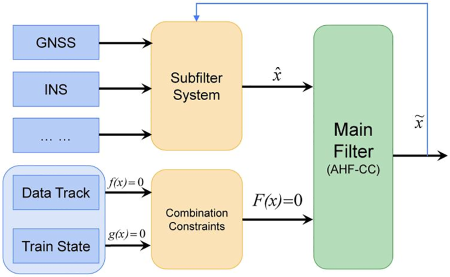
Figure 1: Basic structure of the combination constraint system based on a federated filter

Inertial Navigation System (INS) is an autonomous navigation system that does not rely on external information. The GNSS and other sensors generate a preliminary estimation of the position through the subfilter, and the digital track and train state constraints form a combination constraint. The partly known prior information of the road constraint can be utilized to enhance the tracking performance. Combination constraint and preliminary estimation are used to generate the final constraint position estimation in the main filter [22,23]. The main filter uses the adaptive H∞ filtering algorithm with combination constraint (AHF-CC). The subfilter is updated with the observation and gives the unconstrained estimation. The constraint is applied to give the final estimation [24]. Finally, the train positioning information is fused with other sensors in the form of a combination constraint.

2  Material and Methods

In this section, the precise track constraint method of the train is proposed to improve the accuracy of train positioning. The position constraint of the plane and the train motion state constraints are analyzed.

We can accurately segment the track by continuous fitting and iteration [25]. Then, the railway track can be accurately modeled with a piecewise function to construct a high-precision digital track. Digital track maps will have a constraining effect on trains. The most important constraints are position constraints and motion state constraints. The track plane of railway lines is composed of three types including straight line, transition curve and circular curve, in which transition curve is a cubical parabola [26]. Fig. 2 is a typical precision track from a part of the railway.

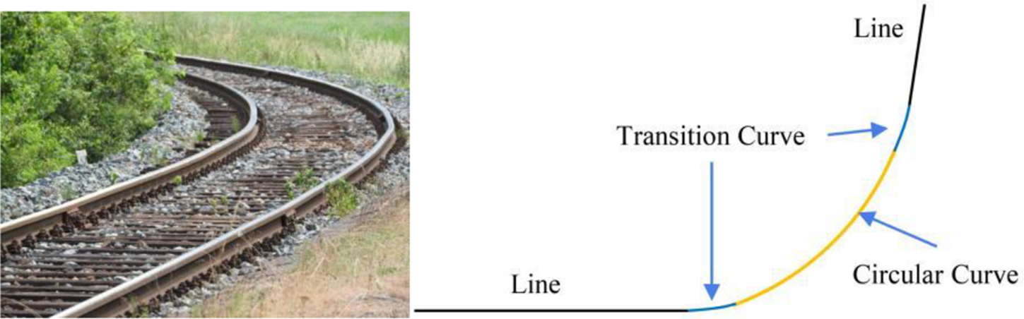
Figure 2: Typical structural diagram of precision track

The essence of train constraint positioning is the fusion of track map information and train position measurement information. The positioning accuracy of the train is improved by the fusion method.

2.1 Linear Constraint Modeling

When a train runs on a straight track segment, the track constraint is the linear constraint. The train is subject to the following linear constraint as [3]

g(x)=Dxk=d,(1)

where D is a given constant, s × n matrix, d is an s × 1 vector and s ≤ n. It is assumed that D has full row rank. If D is not full rank, it means that there are redundant state constraints. A state estimation x^k that satisfies the constraint is expected to get.

2.1.1 Linear Constraint of Linear Railway Track

The coordinates of the points on the railway line are set as (χ, γ). The general equation for the linear model of railway track is as

[k1][χγ]=−b(2)

where k and b represent straight track slope and intercept, respectively.

2.1.2 Linear Constraint of Motion State

The train's running speed, acceleration and heading angle are key parameters of the train's motion state. The state constraints can indirectly improve the accuracy of train position estimation.

The heading angle can reflect the direction of the track in the plane direction [27]. When the train travels on different track segments, the change of heading angle is also different. In the straight segment, the heading angle is a constant value. In the curve segment, the heading angle changes with the mileage. In general, the heading angle may be output by an inertial navigation device, such as an angular rate sensor or magnetic compass. When the satellite signal is good, it can also be obtained by a two-antenna attitude measurement method [28]. The Doppler speed radar equipped on the train has high-speed measurement accuracy, which is about 0.1% of the measured value [29]. A disadvantage of Doppler radar is that its performance depends on environmental conditions, such as weather and the relative motion of ahead objects. The acceleration range of the train is small. According to the requirements of the railway design code [30], the lateral acceleration of running trains on curved tracks is less than 0.75 m/s2 for passengers’ comfort. Taking into account the plane of the track only, the train is subjected to forward acceleration and no lateral acceleration when the train is running in a straight line. When the train is running on the curve track, the train is encountered with forward acceleration and lateral acceleration. The measurement of train acceleration can be obtained through the accelerometer or inertial navigation module, but it needs to pay attention to the influence of cumulative error.

The train state constraint can be written as

[1000010000100001][VeVnaean]=[VDopplersin⁡θINSVDopplercos⁡θINSaINSsin⁡θINSaINScos⁡θINS](3)

where V, a are the forward speed and forward acceleration of the train state estimation, and subscript e, n mean EAST and NORTH. The θINS, Vdoppler, aINS are accurate measurements of the heading angle, forward speed and forward acceleration of the train, which are usually filtered.

2.2 Nonlinear Constraint Modeling

The curved portion of the railway track can be represented by a nonlinear equation, and its constraints on the train are nonlinear constraint. Generally, a nonlinear constraint equation can be written as

f(x)=d(4)

Fig. 3 shows the difference between linear and nonlinear constraints. It indicates the possible error caused by the linear approximation of a nonlinear equality constrained state estimation. Moreover, it shows that the nonlinear constrained state estimation can be projected onto the nonlinear constrained curve, with the resulting error being much smaller than the linearization-introduced error.

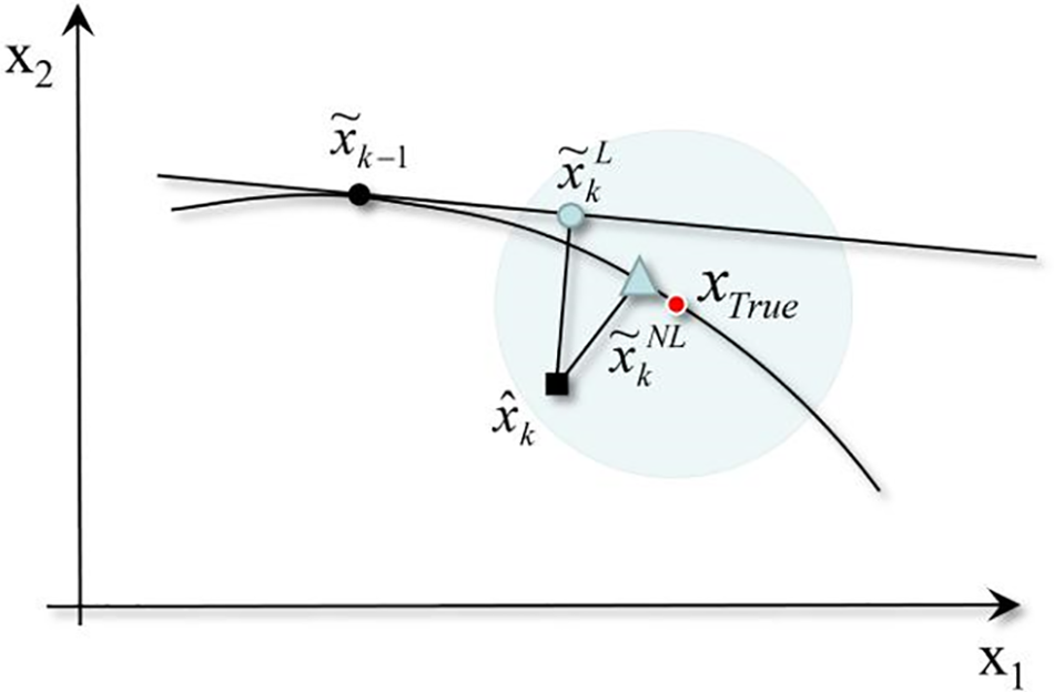
Figure 3: Linear and nonlinear state constraint

In it, x~k−1 is the previous constrained estimation, x^k is the current unconstrained estimation, x~kL is the current linear constrained estimation and x~kNL is the current nonlinear constrained estimation, xTrue is the current true value.

The curve segments of railway lines are composed of circular curves and transition curves. The parametric equation of the circular curve in the independent coordinate system as shown in Fig. 4 can be expressed as

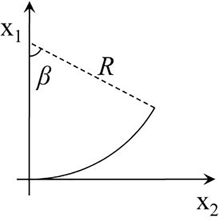
Figure 4: The coordinate of circular curve

{χ=Rsin⁡β,γ=R−Rcos⁡β,β=l/R,(5)

where (χ, γ) is the coordinate of any point on the circular curve. R is the radius of the circular curve. l is the curve length of the point along a circular curve to the point of transition curve to circular on a circular curve. β is the arc angle corresponding to the point.

Taking the center of a circle as the origin of the coordinate, the simplified constraint equation of the circular curve can be expressed as

χ2+γ2=R2(6)

The transition curve is a curved connection between a straight line and a circular curve, whose radius gradually changes from infinity to the radius of a circular curve. In the construction of the railway, the cubical parabola is used to approximate the clothoid [26], and it can be written as

γ=aχ3+bχ2+cχ+d.(7)

Then, the curve line can be expressed as a nonlinear equation

f(x)=0(8)

Furthermore, the nonlinear state constraints about a constrained state estimation x^ are expanded as

fi(x)=fi(x^)+fi′(x^)T(x−x^)+12!(x−x^)Tfi″(x^)(x−x^)+⋯=0(9)

where the superscripts ′,″ denote the first and second partial derivatives.

Ignoring the higher-order of Taylor series expansion, the constraints can be expressed as

f(x)=xTAx+bTx+xTb+c=[xT1][AbbTc][x1]=0(10)

Herein, a railway track segment can be represented by a general equation of the second degree in two variables.

f(χ,γ)=aχ2+2bχγ+cγ2+2dχ+2eγ+f=[χγ1][abdbcedef][χγ1]=0.(11)

2.3 Combination Constraint

Through the analysis above, the constraints of train positioning can be linear or nonlinear, and usually multiple constraints act simultaneously, such as

{gi(x)=xTbi−ci=0fi(x)=0(12)

If the constraint is linear, it can be considered as a special case of the second-order approximate constraint of Eq. (10) (i.e., A = 0).

Therefore, a combination constraint based on multiple constraints is proposed. m represents the number of constraints, and the combined constraint F(x) can be expressed as

F(x)=[f1(x),f2(x),…,fm(x)]T=[xTxT⋱xT][A1A2⋱Am][xx⋮x]+2[b1Tb2T⋮bmT]x+[c1c2⋮cm]=0(13)

3  Results

In the complex operating environment of the train, the statistical characteristics of the actual navigation system noise are difficult to obtain accurately, which leads to the degradation of the performance of the traditional Kalman filter. Therefore, in order to truly reflect the motion of the train, an adaptive filtering algorithm is needed. Considering that H∞ filtering has strong robustness, this paper proposes an adaptive H∞ filtering algorithm with a combination constraint for train positioning, which makes adaptive improvement based on H∞ filter and combination constraint.

3.1 Unconstrained Adaptive H∞ Filter

The state equation and measurement equation of the system are

{xk+1=Fkxk+wkyk=Hkxk+vkzk=Lkxk(14)

where xk is the state variable, Fk is the state transition matrix, Hk is the measurement matrix. wk and vk are system noise and measurement noise, respectively [31]. White noise is not required. The linear combination of state variable zk is the estimated quantity, and Lk is the full rank of the custom estimation matrix.

For the uncertainty of the system model and the statistical characteristics of noise, H∞ filter minimizes the H∞ norm from the interference input to the filtered error output by introducing the H∞ norm idea. This method minimizes the estimation error of the system under the worst-case interference conditions. The cost function of H∞ filtering based on game theory is defined as

J=∑k=1N‖xk−x^k‖2‖x0−x^0‖P0−12+∑k=1N(‖wk‖Qk−12+‖vk‖Rk−12)(15)

where Qk and Rk are the variances of the system noise term and the measurement noise, x0 is the state initial value, P0 is the initial state variance, x^0 is the state estimated value [32].

Generally, it is difficult to minimize J directly, J<1/θ is established by selecting the performance boundary θ. Therefore, at any moment, the H∞ filter needs to meet the following requirement:

Pk−1−θLkTSkLk+HkTRk−1Hk>0(16)

where Pk is the error covariance matrix and Sk is the state variable estimation error covariance matrix. These are pre-set symmetric positive definite matrices. The recursive process of the H∞ filter is

S¯k=LkTSkLkKk=Pk[I−θS¯kPk+HkTRk−1HkPk]−1×HkTRk−1x^k+1=Fkx^k+Kk(yk−Hkx^k)Pk+1=FkPk[I−θS¯kPk+HkTRk−1HkPk]FkT+Qk(17)

The limitation of the filter is that the minimum value of the cost function, J should be satisfied in each iteration computation, which means the condition Eq. (15) should be satisfied.

It can be seen from the recursive Eq. (17) of the H∞ filter algorithm that Kalman filtering is a special case of H∞ filtering. When θ = 0, H∞ filtering is simplified to Kalman filtering. θ is an important factor affecting the robustness of H∞ filtering, which is called the robust factor. The robust factor plays a vital role in the accuracy, robustness and usability of the filter. When the value of the robust factor is too large, the system has high robustness but low filtering accuracy. On the contrary, the value of the robust factor is too small, the stability of the system is weak and even diverges. Therefore, the value of the robust factor directly influences the performance of the filter.

Generally, the robust factor is set to a constant value according to engineering practice experience. Therefore, the filter performance is conservative and cannot adapt to the possible changes in the application environment of the integrated navigation system. It is not guaranteed that the estimation error is small while the system still has strong robustness. Therefore, the selection of robust factors should be adaptively optimized.

Assuming rk is a filter innovation, rk=yk−Hkx^k. rkTrk is the sum of squares of the innovation sequence, which reflects the actual estimation error of the filter.

When rkTrk is large, the performance of the filter is degraded and even diverged. In this case, θ should be appropriately increased. When rkTrk is small, it indicates that the filter estimation accuracy is high, and θ can be appropriately reduced at this time, and the robustness requirement for the filter is reduced to some extent. It can be found that there is a positive proportional relationship between the robust factors θ and rkTrk.

A and B are two n-th order Hermite matrices, A > 0, B ≥ 0, then A>B⇔λ(BA−1)<1. Here λ(A) represents the maximum eigenvalue of A [33].

Then, the following formula can be obtained from the existing condition Eq. (16) of the H∞ filter:

θ<1λ(A),A=LkTLk(Pk−1+HkTHk)−1(18)

θ=1αλ(A),α=1+βrkTrk(19)

The coefficient α > 1, β > 0 are the correlation coefficients, which are generally determined by experiments according to the actual situation of the system.

The H∞ filter updates the robustness factor θ according to the filtering innovation rk continually. This makes the filter adaptive. It can be seen from the comparison that the improved adaptive H∞ filtering cannot only ensure Eq. (15) is established, but also avoid the filter divergence caused by the irrational value of θ, and ensure the automatic adjustment ability of the filter.

3.2 Adaptive H∞ Filter with Combination Constraint

The accuracy of the algorithm is improved by modifying the estimated value through constraints. When the constraint is linear, the unconstrained state estimation of the train at time k is set as x^k. Then the constrained estimation can be written as [34]

x~k=arg⁡minx(x−x^k)TW(x−x^k),(20)

where W is a symmetric positive definite weighting matrix derived from the Lagrangian multiplier technique. Then, the Lagrangian function is expressed as

J(x,λ)=(x−x^k)TW(x−x^k)+2λT(Dx^k−d).(21)

The first order conditions necessary for a minimum are given by

∂J∂x=0⇒W(x−x^k)+DTλ=0,(22)

∂J∂λ=0⇒Dxk−d=0.(23)

Under linear constraint, the solution are given below:

λ=(DW−1DT)−1(Dx^k−d),(24)

x~k=x^k−W−1DT(DW−1DT)−1(Dx^k−d).(25)

The W=Pk−1 or W = I is set to obtain the constrained estimation. Furthermore, the obtained constrained state estimation has a smaller error covariance than that of the unconstrained state estimation, and it is actually the smallest for all constrained filters of this type. Similar results hold in terms of the trace of the estimation error covariance matrix when W = I. The estimations of different constraints with W are shown in Fig. 5.

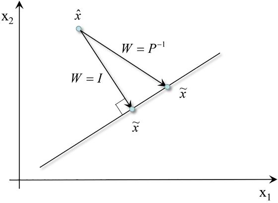
Figure 5: Different constraints with W

When the constraint is a combination of linear and nonlinear constraints, the state estimation of the system under the combination constraint condition (13) can be obtained by using the Lagrange product method. The Lagrangian is expressed as

Φ(x,λ)=(x−x^k)TW(x−x^k)+λTF(x)(26)

where W is any symmetric positive definite weighting matrix, λ=[λ1,λ2,⋯,λm]T is the Lagrangian multipliers vector, and x^ is the unconstrained state estimation. The first-order conditions necessary for a minimum are given by

∂Φ∂x=0⇒W(x−x^k)+∑i=1mλi(Aix+bi)=0(27)

∂Φ∂λ=0⇒F(x)=0.(28)

Assuming that the inverse matrix of W+∑i=1m⁡λiAi exists, the estimation under the combination constraint can be obtained from the above formula:

x~=L−1M(I+∑i=1mλiJi)MTL−1T(Wx^−∑i=1mλibi)(29)

4  Discussion

In this section, three examples are used to verify the effectiveness of the train track and state constrained method and to illustrate the superior performance of combination constrained method compared with unconstrained method.

4.1 Simulation Environment

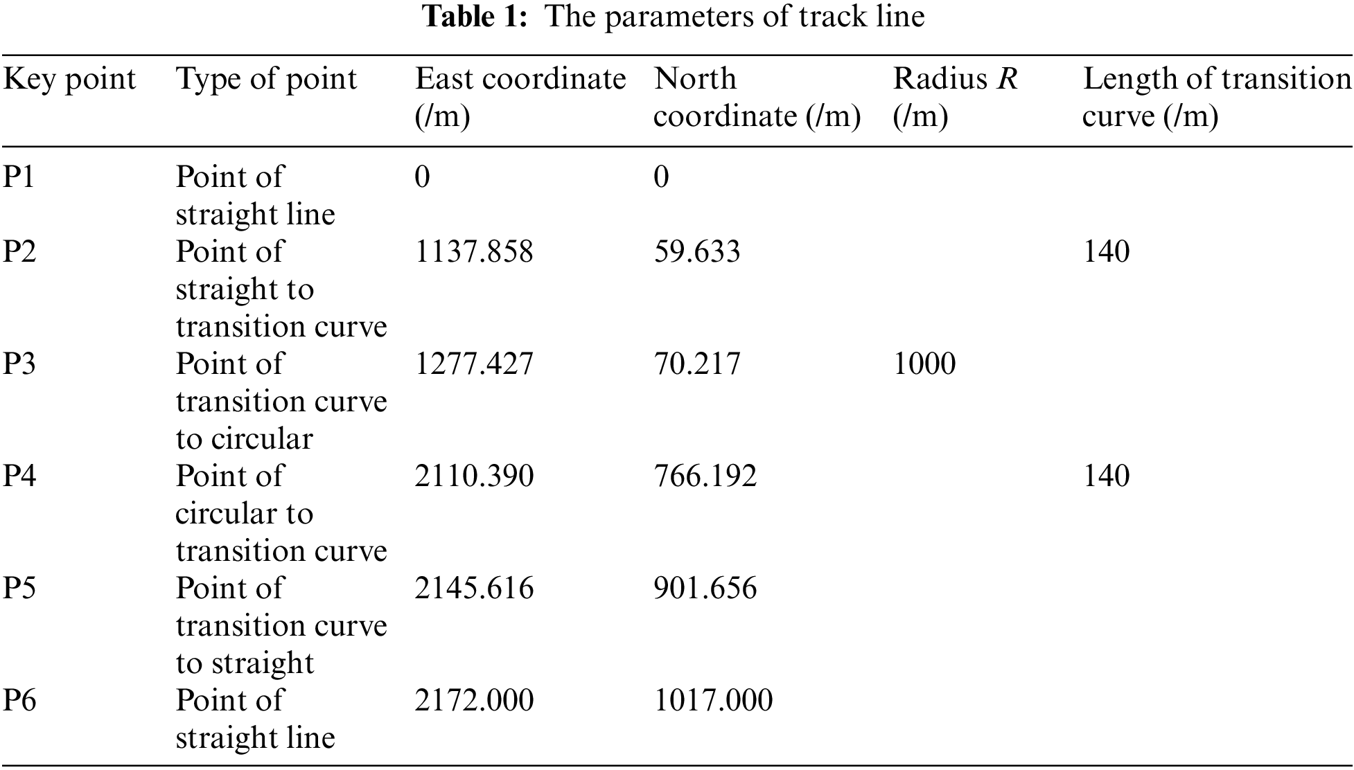
The railway track is part of the Harbin-Dalian Railway and consists of straight and curved segments. The structure of the track is similar to Fig. 2. The radius of the circle is R = 1000 m, and the length of the transition curve is 140 m. The parameters of each segment of the track line are shown in Table 1. The train system state variable is assumed to be x=[xe,x˙e,x¨e,xn,x˙n,x¨n]T, xe,xn represent East location and North location. The target is tracked by GNSS sensor with a sampling interval of T = 1 s. Assuming Q=diag([4,4,1,4,4,1]) and R=diag([100,100]), the initial state of the train is x0=[0,15,0,0,15,0]T, and the corresponding covariance matrix is assumed to be P0=diag([100,4,1,100,4,1]).

In the system simulation, the constraints for comparison are unconstrained AHF, only state-constrained AHF (AHF-SC), only track-constrained AHF (AHF-TC) and the combination constrained AHF (AHF-CC) which act simultaneously with the state constraints and the track constraints. By comparison, the effect of different constraints on the state estimation is analyzed.

Since the discrepancy between the estimated position and the real position is important to the positioning result, in order to compare the effect of the state estimation after adding the constraint information, the root mean square error of the distance (RMSED) is used to evaluate the performance of the algorithm.

RMSED=1M∑k=1M((x^e,k−xe,k)2+(x^n,k−xn,k)2)(30)

where x^e,k,x^n,k represent the EAST and NORTH position estimation of the target state estimation at time k. xe,k,xn,k represent the true eastbound and northbound values of the target at time k. M is the number of positioning points.

4.2 Straight Line Segment Track Simulation

Assume that the train runs at a constant speed on the straight segment track. The angle between the track and the NORTH axis is θ=π/3. The train position is constrained by the railway track. The speed of the train is a constant value V, and acceleration is zero. The train motion state constraints are speed and acceleration. The constraint equations are

{x˙e=Vsin⁡θx˙n=Vcos⁡θ(31)

[100−tan⁡θ000100−tan⁡θ000100−tan⁡θ]x=[000].(32)

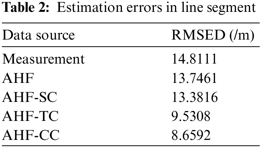
The simulation results of the train positioning are shown in Fig. 6. In Fig. 6, AHF, AHF-SC have a distance from the real track, but AHF-TC, AHF-CC are all on the track line, which mean that the distance errors are small. To accurately understand the distance between the estimated value and the true value, the order of decreasing distance error of AHF, AHF-SC, AHF-TC, AHF-CC are shown in Fig. 7. The constraint performance is analyzed by comparing AHF, AHF-SC, AHF-TC, AHF-CC, measurement and true values.

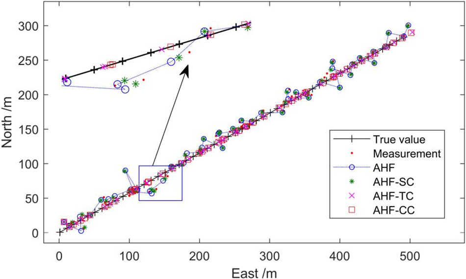
Figure 6: The trajectory simulation diagram of line segment

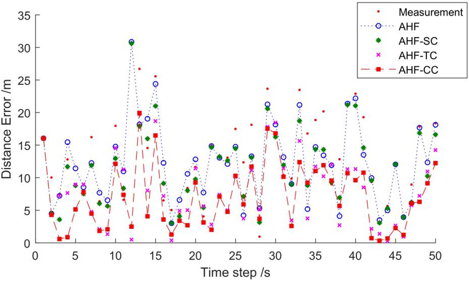
Figure 7: Distance error of linear segment

The evaluation of the constraining effect is listed in Table 2. It can be seen that the constrained filters can significantly outperform the unconstrained counterparts. The effect of AHF-TC is better than that of AHF-SC. Combined with state and track constraints, the AHF-CC can achieve excellent performance and greatly reduce the positioning error.

4.3 Circular Curve Segment Track Simulation

In the second example, train is assumed to travel along a circular road segment with the turn center chosen as the origin of the coordinates and the starting point is (866,500), as shown in Fig. 8. The train is in a state of near uniform motion, and the state constraints of the train are mainly dominated by the heading angle constraint, and the speed and acceleration constraints are negligible. The railway track constraint is quadratic and can be written as

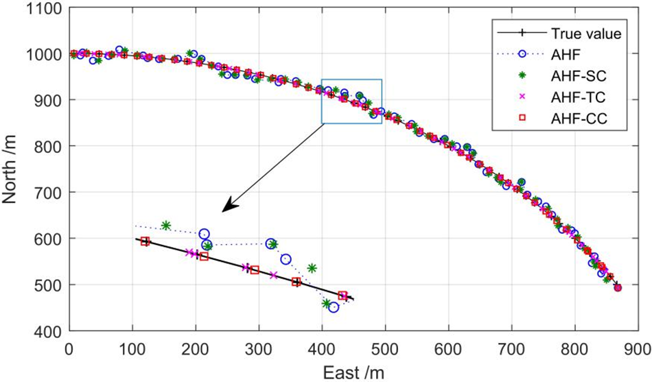
Figure 8: The trajectory simulation of circular curve segment

f(xe,k,xn,k)=xe,k2+xn,k2−R2=[xe,kxn,k][1001][xe,kxn,k]−R2=0(33)

The constraint equation is converted to the form of Eq. (1), that is

[x^e,k00x^n,k000100−tan⁡θk000100−tan⁡θk]x=[R200](34)

where θk is the heading angle of the train at k time. R is the radius of the circle. x^e,k,x^n,k represent the estimated east and north position of the target at time k before the constraint.

The final trajectory simulation result of the train on the circular curve is shown in Fig. 8. The distance between each point and the true point is shown in Fig. 9, and RMSED is listed in Table 3.

Figure 9: Distance error of circular curve segment

It can be seen from Fig. 8 that AHF-TC and AHF-CC with track constraints have better constrained positioning effects. Fig. 9 and Table 3 further demonstrate that AHF-TC performs better than AHF-SC and that the combination constraint has relatively best positioning accuracy. The positioning error is reduced from 12.6906 to 3.9053 m under combination constraint, and the RMSED decreased by about 69% compared to the measurement. The RMSED of AHF-CC is reduced by about 65% compared with AHF. The constraint method of transition curve can refer to the circular curve.

4.4 Full-Line Simulation

In order to better analyze the effect of the combination constraint on improving train positioning accuracy, the simulation results of true value, AHF estimation and AHF-CC estimation are compared in a complete track.

Because there are three types of track segment, the Local Coordinate System (LCS) of each segment is different. The equation of the track is established by the LCS of the track. Therefore, for the convenience of calculation, the train coordinates are converted to LCS of each segment according to the approximations between the measured train coordinates and the segment. Then, the train coordinates are converted to the track System Coordinate System (SCS) after the constraint calculation is completed. The basis for the determination of the approximation principle is the track coordinate range and the train position. The calculation procedure of track constraint from unconstraint point to constraint point is shown in Fig. 10.

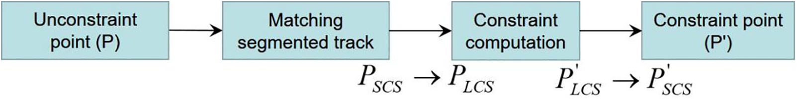
Figure 10: The calculation procedure of track constraint

In Fig. 10, PSCS→PLCS and PLCS′→PSCS′ represent the coordinate transformation between the two coordinate systems. Coordinate transformations include rotation and translation of coordinate. The coordinate transformation equation from the track LCS to the track SCS is

[xe,kSCSxn,kSCS]=[cos⁡α−sin⁡αsin⁡αcos⁡α][xe,kLCSxn,kLCS]+[Oe,mOn,m],(35)

where xe,kSCS,xn,kSCS is the coordinate of the point in the SCS at time k. xe,kLCS,xn,kLCS is the coordinate of the point in the LCS at time k. Oe,k,On,k is the origin coordinate of the m-th segment LCS in the SCS. α is the tangent azimuth of curve starting point in the SCS. The coordinate transformation equation from the track SCS to track LCS is similar to Eq. (35).

The trajectory of the train is calculated and shown in Fig. 11. Fig. 12 is the distance error for the full-line simulation, and Table 4 is the RMSED comparison of the combination constraint and AHF.

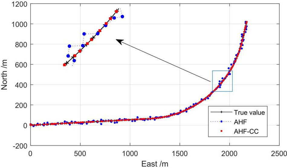
Figure 11: The full-line trajectory of the train

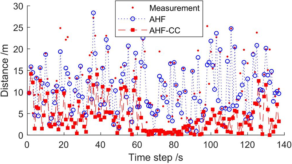
Figure 12: Distance error of the full-line

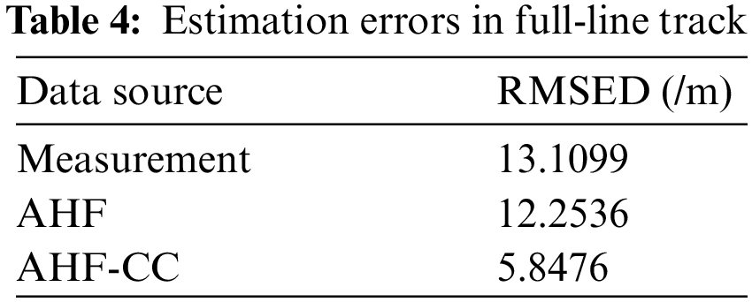
Based on Figs. 11, 12, and Table 4, the full-line RMSED of AHF-CC is reduced by about 52% and 55% compared with AHF and measured value, respectively. The positioning accuracy is relatively high in the curve segment with the time step 62 ~125 s in Fig. 12, which is due to the better effect on the heading angle constraint in the curve segment.

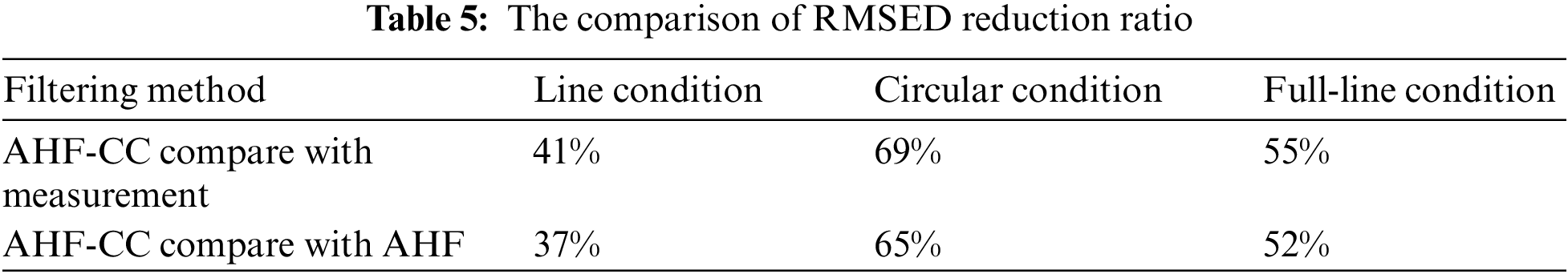
Table 5 shows the results of RMSED reduction ratio in different circumstances between AHF-CC and measurement, AHF, respectively. As shown in Table 5, AHF-CC can improve the positioning accuracy by about one time compared with the measurement and traditional AHF, especially in circular curve segment.

5  Conclusions

In this paper, an adaptive H∞ filtering method for train positioning based on the fusion of prior train information constraints. It melds data from a precise digital track map, prior train status information, and a train positioning sensor. The method can adjust the robust filter parameters autonomously, enhancing the system's robustness and adaptability while preserving the accuracy and stability of the algorithm. Nonlinear track constraints are treated as quadratic constraints, with linear constraints viewed as special cases. Moreover, the combined constrained H∞ filter is derived.

The effectiveness and superiority of the algorithm are confirmed by simulation results. The examples show that the constrained filter is better than the unconstrained filter. The more constraints the system has, the higher accuracy the filter obtains and the higher estimation accuracy the train positioning achieves. The effect of train track constraint is better than that of motion state constraint. The combination constraint with track constraints and motion state constraints can achieve better performance. Compared with the traditional filter, the adaptive H∞ filter with combination constraint can greatly reduce the train positioning error by more than 50%. The nonlinear filtering algorithm and its reliability evaluation under the combination constraint will put forward in further work.

Acknowledgement: The author would like to thank Professor Li Weidong for providing data support, and the financial support mentioned above.

Funding Statement: The authors thank the financial support of the National Natural Science Fund of China (61471080), and Training Plan for Young Backbone Teachers in Colleges and Universities of Henan Province (2018GGJS171).

Author Contributions: The authors confirm contribution to the paper as follows: study conception and design: Xiuhui Diao, Pengfei Wang; data collection: Pengfei Wang; analysis and interpretation of results: Xiuhui Diao, Pengfei Wang, Weidong Li; draft manuscript preparation: Xianwu Chu, Yunming Wang. All authors reviewed the results and approved the final version of the manuscript.

Availability of Data and Materials: The datasets generated and analysed during the current study are not publicly available due to privacy protection reasons but are available from the corresponding author on reasonable request.

Conflicts of Interest: The authors declare that they have no conflicts of interest to report regarding the present study.

References

1. Meng, D. B., Yang, S. Y., Lin, T., Wang, J. P., Yang, H. F. et al. (2022). RBMDO using gaussian mixture model-based second-order mean-value saddlepoint approximation. Computer Modeling in Engineering & Sciences, 132(2), 553–568. https://doi.org/10.32604/cmes.2022.020756 [Google Scholar] [CrossRef]

2. Zhi, P. P., Wang, Z. L., Chen, B. Z., Sheng, Z. Q. (2022). Time-variant reliability-based multi-objective fuzzy design optimization for anti-roll torsion bar of EMU. Computer Modeling in Engineering & Sciences, 131(2), 1001–1022. https://doi.org/10.32604/cmes.2022.019835 [Google Scholar] [CrossRef]

3. Simon, D. (2010). Kalman filtering with state constraints: A survey of linear and nonlinear algorithms. IET Control Theory and Applications, 4(8), 1303–1318. [Google Scholar]

4. Zhu, S. P., Liu, Q., Zhou, J., Yu, Z. Y. (2018). Fatigue reliability assessment of turbine discs under multi-source uncertainties. Fatigue & Fracture of Engineering Materials & Structures, 41(6), 1291–1305. [Google Scholar]

5. Karim, E. M., Serge, R., Jean-Bernard, C., Georges, S., Benaissa, A. et al. (2017). Circular particle fusion filter applied to map matching. IET Intelligent Transport Systems, 11(8), 491–500. [Google Scholar]

6. Meng, D. B., Yang, S. Y., He, C., Wang, H. T., Lv, Z. Y. et al. (2022). Multidisciplinary design optimization of engineering systems under uncertainty: A review. International Journal of Structural Integrity, 13(4), 565–593. [Google Scholar]

7. Meng, D. B., Yang, S. Y., de Jesus, A. M. P., Zhu, S. P. (2023). A novel Kriging-model-assisted reliability-based multidisciplinary design optimization strategy and its application in the offshore wind turbine tower. Renewable Energy, 203(C), 407–420. [Google Scholar]

8. Mokhtari, K. E., Reboul, S., Azmani, M., Choquel, J. B., Benjelloun, M. (2014). A map matching algorithm based on a particle filter. International Conference on Multimedia Computing & Systems, pp. 723–727. Marrakesh, Morocco, IEEE. [Google Scholar]

9. Meng, D. B., Yang, S. Y., Zhang, Y., Zhu, S. P. (2019). Structural reliability analysis and uncertainties-based collaborative design and optimization of turbine blades using surrogate model. Fatigue & Fracture of Engineering Materials & Structures, 42(6), 1219–1227. [Google Scholar]

10. Park, G., Hwang, Y., Choi, S. B. (2017). Vehicle positioning based on velocity and heading angle observer using low-cost sensor fusion. Journal of Dynamic Systems, Measurement, and Control, 139(12), 121008. [Google Scholar]

11. Neri, A., Sabina, S., Capua, R., Salvatori, P. (2016). Track constrained RTK for railway applications. 29th International Technical Meeting of the Satellite Division of the Institute of Navigation, pp. 2123–2135. Portland, USA. [Google Scholar]

12. Liu, J., Cai, B. G., Wang, J. (2016). Track-constrained GNSS/odometer-based train localization using a particle filter. International Intelligent Vehicles Symposium, pp. 877–882. Gotenburg, Sweden, IEEE. [Google Scholar]

13. Zhi, P. P., Xu, Y., Chen, B. Z. (2020). Time-dependent reliability analysis of the motor hanger for EMU based on stochastic process. International Journal of Structural Integrity, 11(3), 453–469. [Google Scholar]

14. Yamamoto, H., Takasu, T., Kubo, N. (2015). Multi-GNSS based train positioning constrained by three-dimensional track coordinates. Journal of the Institute of Positioning, Navigation and Timing of Japan, 6(3), 12–21. [Google Scholar]

15. Wang, P., Diao, X. (2022). Beidou GPS/SINS satellite positioning system based on embedded operating system. International Journal of Embedded Systems, 15(3), 259–269. [Google Scholar]

16. Zhao, Y. (2016). Performance evaluation of Cubature Kalman filter in a GPS/IMU tightly-coupled navigation system. Signal Processing, 119(1), 67–79. [Google Scholar]

17. Kim, K., Seol, S., Kong, S. H. (2015). High-speed train navigation system based on multi-sensor data fusion and map matching algorithm. International Journal of Control Automation and Systems, 13(3), 503–512. [Google Scholar]

18. Joerg, S., Silvia, B., Federico, R. (2016). Map-matching algorithm applied to bicycle global positioning system traces in bologna. IET Intelligent Transport Systems, 10(4), 244–250. [Google Scholar]

19. Rohani, M., Gingras, D., Gruyer, D. (2015). A novel approach for improved vehicular positioning using cooperative map matching and dynamic base station DGPS concept. IEEE Transactions on Intelligent Transportation Systems, 17(1), 230–239. [Google Scholar]

20. Frikha, A., Moalla, H. (2015). Analytic hierarchy process for multi-sensor data fusion based on belief function theory. European Journal of Operational Research, 241(1), 133–147. [Google Scholar]

21. Li, Z., Gao, J., Wang, J., Yao, Y. (2017). PPP/INS tightly coupled navigation using adaptive federated filter. GPS Solutions, 21(1), 137–148. [Google Scholar]

22. Zhang, Z. H., Li, K. Y., Zhou, G. J. (2018). State estimation with a heading constraint. 2018 International Conference on Information Fusion, pp. 253–258. Cambridge, UK. [Google Scholar]

23. Teixeira, B. O. S., Chandrasekar, J., Tôrres, L. A. B., Aguirre, L. A., Bernstein, D. S. (2009). State estimation for linear and non-linear equality-constrained systems. International Journal of Control, 82(5), 918–936. [Google Scholar]

24. Xu, L., Li, X. R., Liang, Y., Duan, Z. (2017). Constrained dynamic systems,generalized modeling and state estimation. IEEE Transactions on Aerospace and Electronic Systems, 53(5), 2594–2609. [Google Scholar]

25. Wang, P. F., Li, W. D. (2023). Indoor and outdoor seamless positioning technology based on artificial intelligence and intelligent switching algorithm. Wireless Communications and Mobile Computing, 2023(2), 7075834. [Google Scholar]

26. TB10098-2017 (2017). Code for design of railway line. Beijing, China: China Railway Press. [Google Scholar]

27. Chen, Q., Niu, X., Zhang, Q., Cheng, Y. (2015). Railway track irregularity measuring by GNSS/INS integration. Navigation, 62(1), 83–93. [Google Scholar]

28. Zhao, L., Li, N., Li, L., Zhang, Y., Cheng, C. (2017). Real-time GNSS-based attitude determination in the measurement domain. Sensors, 17(2), 296 [Google Scholar] [PubMed]

29. Cui, K., Dong, C. (2017). Analysis of the safety integrity in integrated train speed measurement system. Urban Mass Transit, 20(7), 65–68. [Google Scholar]

30. TB10621-2014 (2014). Code for design of high speed railway. Beijing, China: China Railway Press. [Google Scholar]

31. Uribe-Murcia, K., Shmaliy, Y. S., Andrade-Lucio, J. A. (2021). Unbiased FIR, kalman, and game theory H∞ filtering under bernoulli distributed random delays and packet dropouts. Neurocomputing, 442(7), 89–97. [Google Scholar]

32. Zhang, T., Deng, F., Zhang, W. (2021). Robust H-infinity filtering for nonlinear discrete-time stochastic systems. Automatica, 123, 109343. [Google Scholar]

33. Xie, L. Q., He, L. M., University, S. (2015). Ensemble kalman filter with state equality constraints. Journal of Sichuan University (Natural Science Edition), 52(5), 958–962. [Google Scholar]

34. Wang, P. F., Li, W. D., Wang, X. P., Chu, X. W., Liu, Y. (2021). Adaptive multi-model H∞ filter postioning algorithm about train. Control Engineering of China, 28(1), 135–141. [Google Scholar]