
 Submit a Paper
 Propose a Special lssue
 Open Access
ARTICLE

Gradient Optimizer Algorithm with Hybrid Deep Learning Based Failure Detection and Classification in the Industrial Environment
1 Department of Electrical and Computer Engineering (ECE), King Abdulaziz University, Jeddah, 21589, Saudi Arabia
2 Center of Excellence in Intelligent Engineering Systems (CEIES), King Abdulaziz University, Jeddah, 21589, Saudi Arabia
3 Department of Nuclear Engineering, King Abdulaziz University, Jeddah, 21589, Saudi Arabia
4 Department of Electrical and Electronic Engineering, Rajshahi University of Engineering and Technology, Rajshahi, Bangladesh
* Corresponding Author: Ibrahim M. Mehedi. Email:
(This article belongs to the Special Issue: Failure Detection Algorithms, Methods and Models for Industrial Environments)
Computer Modeling in Engineering & Sciences 2024, 138(2), 1341-1364. https://doi.org/10.32604/cmes.2023.030037
Received 20 March 2023; Accepted 06 July 2023; Issue published 17 November 2023
 View Full Text
 Download PDF
Abstract
Failure detection is an essential task in industrial systems for preventing costly downtime and ensuring the seamless operation of the system. Current industrial processes are getting smarter with the emergence of Industry 4.0. Specifically, various modernized industrial processes have been equipped with quite a few sensors to collect process-based data to find faults arising or prevailing in processes along with monitoring the status of processes. Fault diagnosis of rotating machines serves a main role in the engineering field and industrial production. Due to the disadvantages of existing fault, diagnosis approaches, which greatly depend on professional experience and human knowledge, intellectual fault diagnosis based on deep learning (DL) has attracted the researcher’s interest. DL reaches the desired fault classification and automatic feature learning. Therefore, this article designs a Gradient Optimizer Algorithm with Hybrid Deep Learning-based Failure Detection and Classification (GOAHDL-FDC) in the industrial environment. The presented GOAHDL-FDC technique initially applies continuous wavelet transform (CWT) for preprocessing the actual vibrational signals of the rotating machinery. Next, the residual network (ResNet18) model was exploited for the extraction of features from the vibration signals which are then fed into the HDL model for automated fault detection. Finally, the GOA-based hyperparameter tuning is performed to adjust the parameter values of the HDL model accurately. The experimental result analysis of the GOAHDL-FDC algorithm takes place using a series of simulations and the experimentation outcomes highlight the better results of the GOAHDL-FDC technique under different aspects.Keywords
Industrial system integration and information technology seem to be increasing due to the tremendous growth of advanced industry, highly reliable systems and components are the assurance for the safe operation of aerospace [1]. Hidden aviation faults might result in catastrophic actions of aviation machinery. Since the building blocks of aircraft engines, space shuttles, and other rotating machines, the mechanical transmission technique is inclined to different faults under harsh operating, heavy load conditions, and high speed for a longer time directly affects the safe operation of the mechanical technique [2]. The rotating machinery denoted by aviation equipment has gained popularity among researcher workers. Earlier fault diagnosis and detection (FD) techniques could forecast the fault growth trend that had a main role in preventing mechanical engineering transmission system faults [3]. Thus, every industry attaches considerable attention to the intelligent FD technique on rotating machinery to prevent the existence of succeeding major accidents caused by minor faults [4]. FD of rotating machinery is a method of FD, identification, and isolation that is employed on the data about the operational condition of the equipment. There are three fundamental tasks of FD: (1) find the incipient failure and its reason; (2) forecast the trend of fault growth; (3) determine whether the equipment is normal or not [5]. Thus, essentially, FD is considered a pattern recognition problem with respect to the rotating machinery condition.
As a robust pattern recognition method, artificial intelligence (AI) has gained popularity among several researcher workers and shows efficacy in rotating machinery FD applications [6]. Because of the richness and variability of the response signal, it is not possible to directly identify fault patterns. Thus, a typical FD technique often involves two main stages: fault recognition, and data processing (feature extraction) [7]. The most common intelligent FD system is constructed by using the preprocessing by feature extraction algorithm to convert the input pattern such that they can be denoted by low-dimension feature vectors for easy comparison and match [8]. Several AI techniques or tools were applied involving convex optimization, and mathematical optimization, along with probability-, classification- and statistical learning-based techniques [9]. Especially, statistical learning methods and classifiers were extensively exploited in FD of rotating machinery, which involves support vector machine (SVM), artificial neural network (ANN), k-nearest neighbor (KNN), and Bayesian classifier. Previously, deep learning (DL) methods have begun to be employed in the field of FD [10]. Based on the modern advances in DL algorithm, most of the AI technology lack of explainability traits and they need a massive amount of data labeled for fault and normal conditions, drastically limiting the industrial applications.
The motivation behind the proposed model is to bring advancements in industrial processes through sensor-based data collection for monitoring and fault detection. However, traditional fault diagnosis approaches still rely on human expertise and have limitations in accuracy and scalability. Therefore, there is a need for novel approaches that leverage the power of advanced technologies such as deep learning and optimization algorithms to improve fault diagnosis in the industrial environment.
The following are the contributions, and it is included in the introduction section:
In this article, we present a novel approach called the Gradient Optimizer Algorithm with Hybrid Deep Learning-based Failure Detection and Classification (GOAHDL-FDC) for accurate fault detection and classification in the industrial environment. Our approach combines several existing theoretical knowledge and techniques, including Continuous Wavelet Transform (CWT), Residual Network (ResNet18) model, Hybrid Deep Learning (HDL), and Gravitational Optimization Algorithm (GOA), in a unique and synergistic way to overcome the limitations of existing fault diagnosis approaches. The contributions of this work can be summarized as follows:
Design of GOAHDL-FDC technique: We propose a novel technique that integrates CWT for preprocessing, ResNet18 for feature extraction, HDL for automated fault detection, and GOA for hyperparameter tuning. This unique combination of techniques aims to improve the accuracy and effectiveness of fault detection and classification in the industrial environment.
Addressing limitations of existing approaches: Our GOAHDL-FDC technique is designed to overcome the limitations of traditional fault diagnosis approaches that rely on human expertise, may lack scalability, incomplete feature extraction, limited hyperparameter tuning, and insufficient utilization of optimization techniques. By leveraging advanced deep learning and optimization techniques, our approach aims to provide a more accurate and scalable solution for fault diagnosis in the industrial environment.
Experimental result analysis: We conduct a series of simulations and experiments to evaluate the performance of the GOAHDL-FDC technique. The outcomes of the experimentation highlight the effectiveness and superiority of our approach compared to existing methods, showcasing the potential of our proposed approach for modern data-driven applications in Industry 4.0.
This article designs a Gradient Optimizer technique with Hybrid Deep Learning-based Failure Detection and Classification (GOAHDL-FDC) in the industrial environment. The presented GOAHDL-FDC technique initially applies continuous wavelet transform (CWT) to preprocess the actual vibrational signals of the rotating machinery. Next, the residual network (ResNet18) method was used for the extraction of features from the vibration signals, which are then fed into the HDL model for automated fault detection. Finally, the GOA based hyper parameter tuning process was performed to adjust the parameter values of the HDL model accurately. The experimental validation of the GOAHDL-FDC approach is carried out using a series of simulations.
Zhao et al. [11] proposed a novel FD technique by using Local-Global DNN (LGDNN) algorithm. Initially, this FD method could directly apply the presented technique for extracting global and local structural features from the original vibration spectral signal. Then, the highest level feature which is extracted was employed for classifying the different fault conditions based on the Softmax classifier. Li et al. [12] developed a DL-related domain generalization technique for FD machinery. The presented method is adopted for expanding the presented data. Domain adversarial training was performed, and generalized features are learned from distinct domains that hold in new working scenarios without considering the availability of the testing dataset. Also, distance metric learning is utilized for further enhancing the robustness of the model in fault classification.
Gong et al. [13] introduced a novel CNN-SVM technique. This technique enhances the traditional CNN architecture by presenting the global average pooling technique and SVM. Initially, the spatial and temporal multi-channel raw information from different sensors was inputted directly towards the enhanced CNN-Softmax architecture for training the CNN technique. Next, the enhanced CNN is applied to the extra representation feature from the raw fault information. Lastly, the derived sparse representation feature vector was inputted into SVM for the classification of the fault. In [14], an innovative technique grounded on RNN was developed for identifying the type of fault in rotating machinery. Next, GRU is proposed for exploiting temporal data of time-series datasets and learning representation features from built images. Finally, an MLP is applied for implementing FD. Yongbo et al. [15] designed a FD technique with CNN for InfRared Thermal (IRT) images. Initially, the IRT method is applied to capture the IRT images of rotating machinery. Next, the CNN is exploited for extracting fault features from the IRT image. Lastly, the attained feature was given into the Softmax Regression (SR) classifiers for fault pattern detection.
Surendran et al. [16] proposed an Intelligent Industrial FD with Sailfish Optimized Inception using Residual Network (IIFD-SOIR). The presented method exploits a Continuous Wavelet Transform (CWT) for pre-processed representation of the original vibration signal. Additionally, the parameter tuning of Inception including the ResNet v2 method is implemented by the sailfish optimizers. Lastly, an MLP is exploited as a classification method for proficiently diagnosing the fault. Liu et al. [17] devised a technique integrating a 1D-CNN and 1D denoising convolutional autoencoder (DCAE) for addressing these problems, where the initial one is applied for the noise reduction of raw vibration signal and the next one is applied for FD using the denoised signal.
The study by [18] presented a novel approach for analyzing the random vibration of bridges under the influence of vehicle dynamic interaction. The authors propose a Bayesian deep learning approach, which combines deep learning techniques with Bayesian inference, to accurately predict the response of bridges to random vibrations caused by vehicles. The proposed approach takes into account the uncertainties associated with bridge parameters, vehicle loadings, and environmental conditions, and provides probabilistic predictions of bridge responses, which are crucial for ensuring the safety and reliability of bridges. The study addresses a critical issue in the field of bridge engineering, as the dynamic interaction between bridges and vehicles can cause significant vibrations that can potentially lead to structural damage or failure. By incorporating Bayesian inference into deep learning, the proposed approach provides a probabilistic framework that captures the uncertainties in the analysis, making it more robust and reliable compared to traditional deterministic methods.
By observing the following are the shortcomings of the existing approaches: Reliance on human expertise: Traditional fault diagnosis approaches in the industrial environment heavily depend on professional experience and human knowledge, which may result in subjective and less accurate results. Lack of scalability: Existing methods may not be scalable enough to handle large amounts of data from modern industrial processes equipped with numerous sensors, leading to limitations in real-time or near-real-time fault detection and classification.
Incomplete feature extraction: Feature extraction, which is crucial for accurate fault diagnosis, may not be optimized in existing methods, leading to suboptimal performance.
Limited hyperparameter tuning: Hyperparameters of deep learning models used for fault diagnosis may not be properly tuned, leading to suboptimal model performance and limited accuracy. Insufficient utilization of optimization techniques: Existing approaches may not fully utilize advanced optimization techniques for hyperparameter tuning, leading to suboptimal performance of the deep learning models.
The proposed approach in the title aims to address these limitations by introducing a novel gradient optimizer algorithm and leveraging hybrid deep learning techniques, with a focus on improving fault diagnosis in the industrial environment. The proposed method was trained by the noisy input for denoising learning. In this proposed method, a global average pooling layer, rather than an FC layer is exploited as a classifier for reducing the risk of overfitting and the amount of parameters.
In this article, we have focused on the design of the GOAHDL-FDC technique for accurate failure detection and classification in the industrial environment. The presented GOAHDL-FDC technique encompasses a series of operations such as CWT-based preprocessing, ResNet feature extraction, HDL-based failure detection, and GOA-related hyperparameter tuning.
In this article, the design of the GOAHDL-FDC technique for accurate failure detection and classification in the industrial environment is focused and the following reasons, the proposed model overcomes the existing model.
“Gradient Optimizer Algorithm”: The proposed algorithm incorporates a gradient optimizer, specifically the Gravitational Optimization Algorithm (GOA), for hyperparameter tuning of the Hybrid Deep Learning (HDL) model. This introduces a new optimization approach for improving the performance of the HDL model in the context of failure detection and classification in industrial systems.
“Hybrid Deep Learning-based Failure Detection and Classification”: The proposed approach combines the power of deep learning techniques, specifically the continuous wavelet transform (CWT) for preprocessing and a residual network (ResNet18) model for feature extraction, with the GOA-based hyperparameter tuning. This hybrid approach brings together different deep-learning components to create a novel solution for failure detection and classification in the industrial environment.
“Improved Fault Diagnosis in an industrial environment”: The proposed approach is specifically designed for the context of Industry 4.0, which refers to the modernization and digitization of industrial processes. By leveraging deep learning and optimization techniques, the proposed approach aims to improve fault diagnosis in industrial systems, addressing the limitations of existing approaches that rely heavily on human expertise and knowledge. Overall, the title highlights the novelty of the proposed approach, which combines a gradient optimizer algorithm, hybrid deep learning techniques, and a focus on Industry 4.0 for improved failure detection and classification in the industrial environment. Fig. 1 represents the overall process of GOAHDL-FDC method.
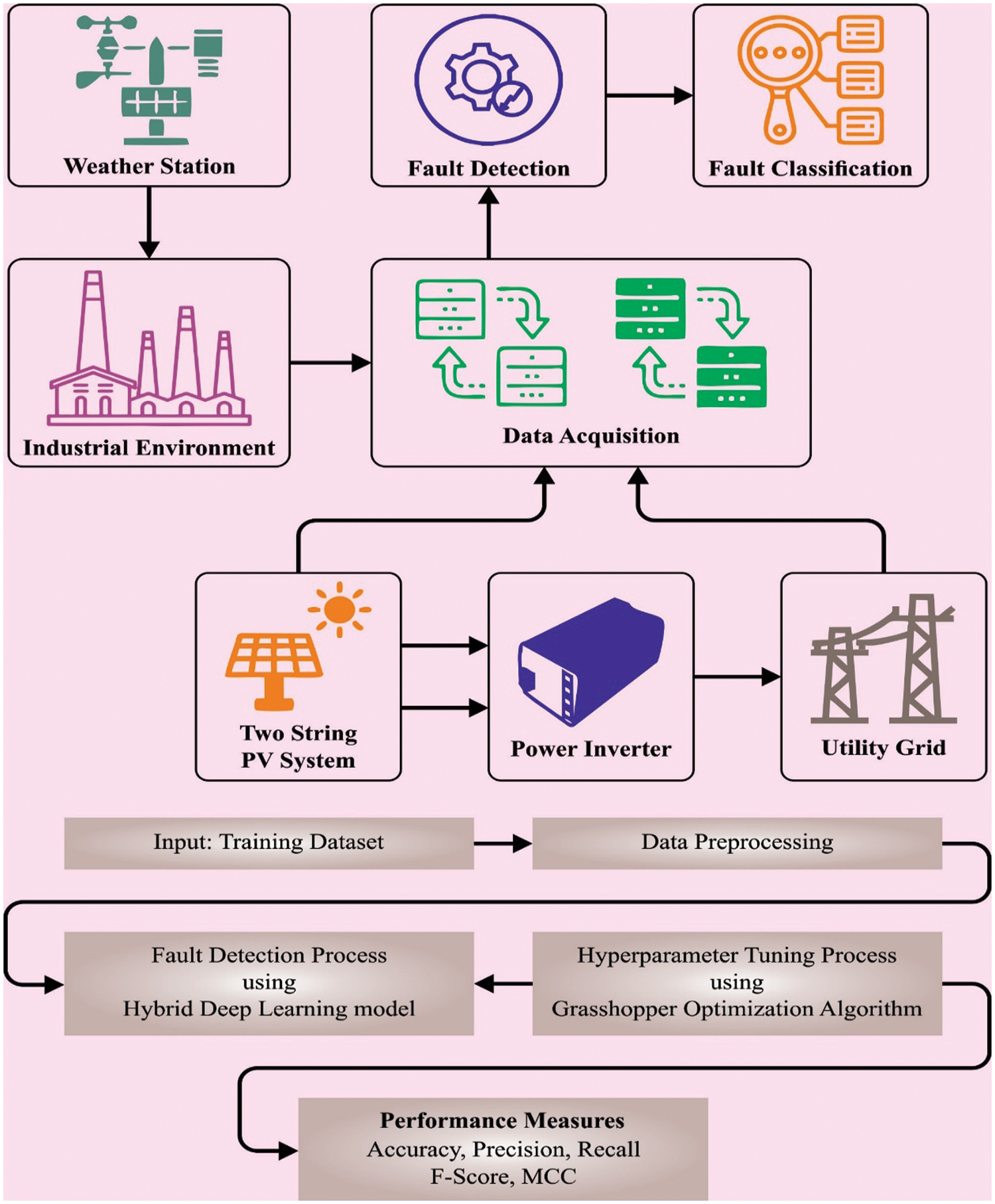
Figure 1: Overall process of GOAHDL-FDC approach
3.1 Data Preprocessing and Feature Extraction
Rotating machinery is a process of several rotating speeds and loads. In order to execute fault detection in any working conditions, the vibration signal from machine in complete speed range and load was crucial to gain for training it [19]. Primarily, the vibration signal was get together in rotating speed database. Specially, the rotating speed from trained case is considered that constant as it could be together once the machinery is constant working method. The CWT maintains and creates the localization proposal of STFT. The CWT of signal
whereas
Attaining every wavelet coefficient in matrix
In which
Then, the features are extracted by the use of ResNet-18 model. ResNet is a CNN that removes particular layers in the network using skip connection. The skip connection decreases the training time and helps to resolve the challenges of gradient disappearing in the CNN. The nonlinear activation function is applied between the skipped layers. Also, BN function is used between the shortcut connections. A weight matrix is applied which evaluates the weight of jump connection. In the later stage of the network, the expansion is applied, afterward learning the feature of the input. Many instances of the residual block are applied all over the network. The mapping from
In the network, the resultant residual blocks for the stacked layer with a similar dimension are provided using Eq. (3).
During the training, the function
3.2 Failure Detection Using HDL Model
In this work, the HDL model is applied to the failure detection process in rotating machinery [20]. LSTM mechanism on the backpropagation (BP) rule as it should compute gradients for the procedure optimizer. Its variations are weighted based on the rate of errors it computes at every cell level. LSTM is accomplished sufficient for learning long-term dependencies over a long time utilizing its memory unit. The main element of LSTM is the cell state. It goes straight down the whole time steps with only minor however vital connections. LSTM is remove or adds data in the cell state utilizing many gates. All the gates develop a sigmoid NN layer. These sigmoid layers create output numbers between zero and one, which signifies that several data of all the components are supposed to be allowed.
Assume the subsequent diagram for understanding the LSTM structure. LSTM contains 3 functions gates are:
• Forget gate
• Input gate
• Output gate
whereas,
The sigmoid of multiplication of the input additional with bias value occurred. This layer supports returning zero and one if it is require this data from predictive or not. The next gate is input gate, assume the under declared formula.
A primary part of input layer formula is like the formula of forget gate, rather than being the weight and bias. It endures a sigmoid function. During the next 2 formulas, it manages that part to add a cell state utilizing
GRU is considered the variant of LSTM. It contains 3 sigmoid layers as tanh layer, update gate, and reset gate. Assume the attached diagram to optimum realizes the formulas. The GRU utilizes the reset and update gates for vanishing gradient issues and these support in determining the outcome. A primary point of this technique was update gate. Initially, the subsequent equation computes update gate
whereas
Computation begins if
The estimate starts with augmentation of data
From the calculation, once the vector
Considering the technique from left to right. The method composed of LSTM layers, bidirectional layers, GRU layers considered feed-forward, to better train and predict the price values and electrical load precisely. LSTM layer is the input normalized features presented to the first layer and training inputted features in feed-forward way. GRU layer is applicable in the bidirectional layer. Initially, it goes through training in feed-forward manner than in feed backward manner. The hybrid layer comprising layers of LSTM and GRU in a given manner is enriching the predictions accuracy of the predictive techniques. A dropout layer to avoid overfitting, followed by a bidirectional GRU layer, follows the LSTM Layer. From all input neurons, the dense layer which is connected deeply receives the output.
3.3 Hyperparameter Tuning Using GOA
Finally, the GOA based hyperparameter tuning process was performed to adjust the parameter values of the HDL model accurately. GOA is the newly developed algorithm that has two mechanisms: local escaping operator and gradient search rule [21]. Fig. 2 illustrates the flowchart of GOA.
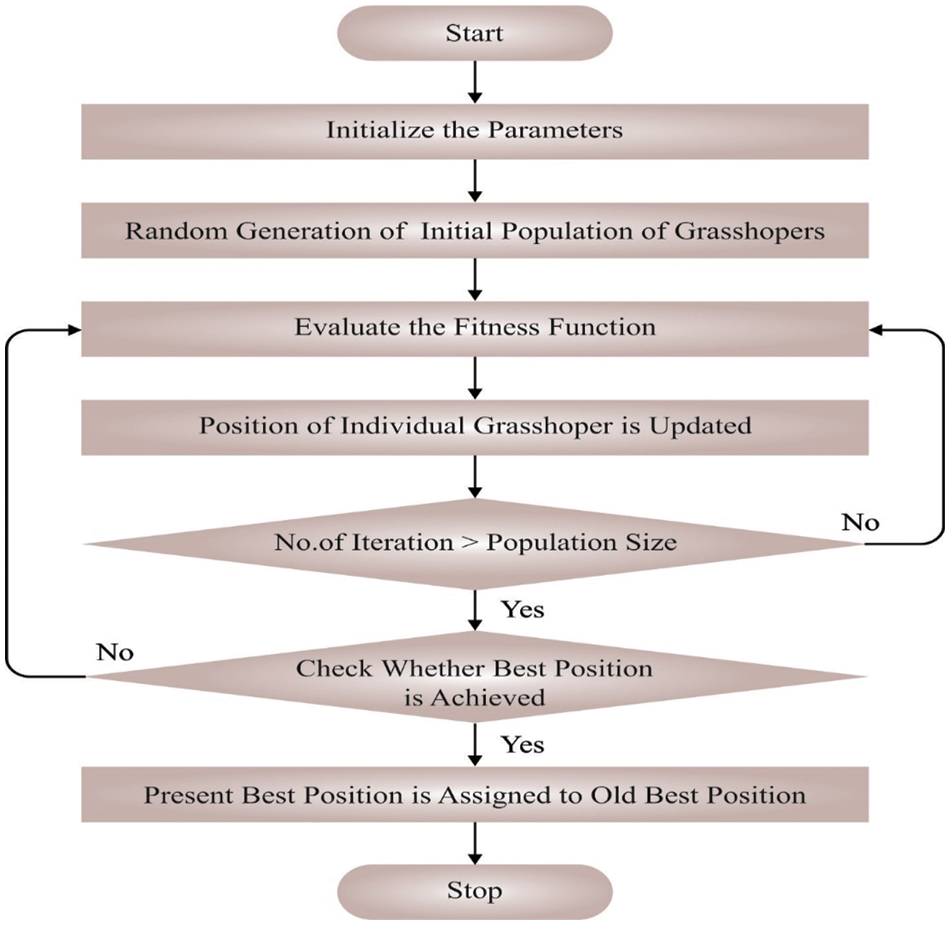
Figure 2: Flowchart of GOA
During the optimization process, the presented
In Eq. (14),
where
where
The novel vector
where
The newly generated solution at the following iteration
A local escaping operator (LEO) is proposed for increasing the efficacy of GOA. The LEO generates a solution with better performance
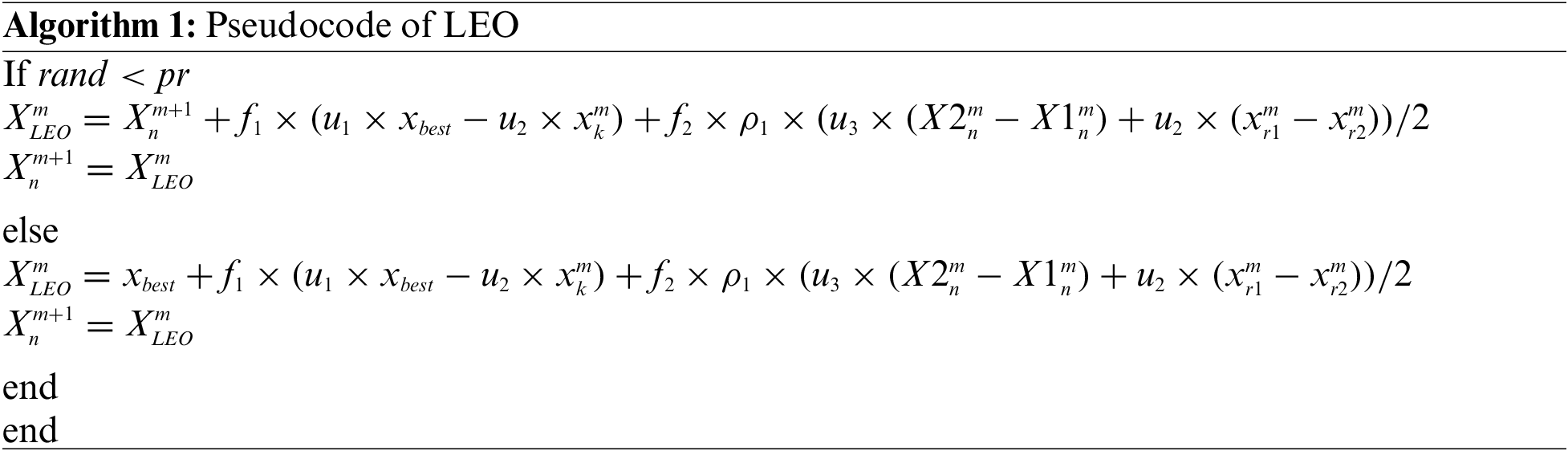
where
If parameter
where
In Eq. (32), if
where
The performance of the GOAHDL-FDC technique is experimentally authenticated using automotive gearbox [22] and bearing [23] fault dataset. The previous dataset covers seven classes where the latter dataset contains 10 classes. The primary dataset has seven different kinds of health statuses, like three kinds of compound faults (Missing tooth (0.2 mm), Normal, Minor-chipped tooth, and missed tooth gear fault, outer race-bearing fault, the Missing tooth (2 mm) and minor-chipped gear fault. The second dataset includes normal along with fault data. The bearing fault has some kinds, like the Ball faults (BF), Inner race (IF), and Outer race (OF).
In this article, we present the Gradient Optimizer Algorithm with Hybrid Deep Learning-based Failure Detection and Classification (GOAHDL-FDC) for accurate fault detection and classification in the industrial environment. To ensure a fair comparison with existing methods, we have carefully designed the experimental setup, including the selection of hyperparameters, the number of repeated experiments, and the evaluation of stability and complexity of our proposed model.
Experimental Setup:
Hyperparameter tuning: We utilize the Gravitational Optimization Algorithm (GOA) for hyperparameter tuning of the HDL model in our GOAHDL-FDC technique. The hyperparameters, such as learning rate, batch size, and number of hidden layers, are carefully selected based on empirical studies and domain expertise. We conduct a systematic search over a range of hyperparameter values to optimize the performance of our model.
Number of repeated experiments: To ensure the robustness and reliability of our results, we conduct multiple repeated experiments with different random seeds. The number of repeated experiments is determined based on statistical considerations and typically ranges from 5 to 10, depending on the complexity of the dataset and the computational resources available.
Evaluation of stability and complexity: To assess the stability of our proposed model, we calculate the standard deviation of accuracy for the repeated experiments. A lower standard deviation indicates higher stability and consistency in the performance of our model. Additionally, we evaluate the complexity of our model in terms of time-consuming. We measure the runtime of our GOAHDL-FDC technique for different datasets and compare it with existing methods to assess its computational efficiency.
In Table 1 and Fig. 3, the experimental results of the GOAHDL-FDC approach are studied under 70:30 of TRP/TSP of gearbox dataset. The average result analysis reported that the GOAHDL-FDC technique identifies all kinds of faults in the gearbox dataset. For instance, with 70% of TRP, the GOAHDL-FDC technique attains average
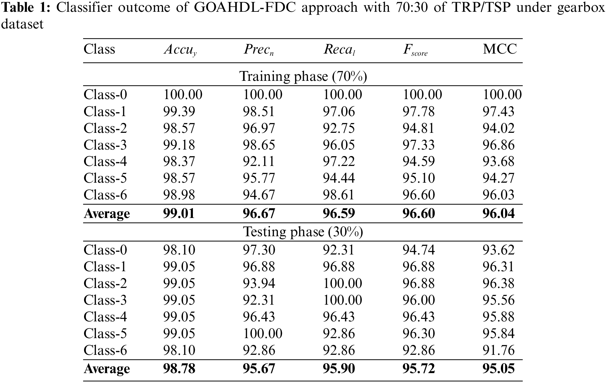
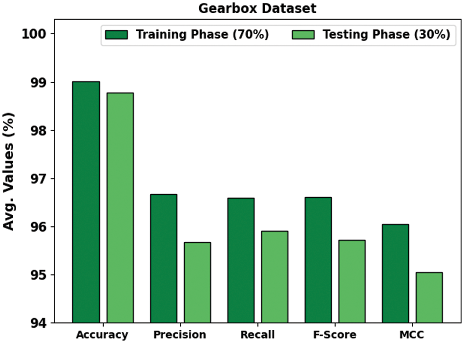
Figure 3: Average outcome of GOAHDL-FDC approach with 70:30 of TRP/TSP under gearbox dataset
In Table 2 and Fig. 4, the experimental results of the GOAHDL-FDC approach are studied under 80:20 of TRP/TSP of gearbox dataset. The average result analysis stated that the GOAHDL-FDC technique identifies all kinds of faults in the gearbox dataset. For example, with 80% of TRP, the GOAHDL-FDC technique attains average
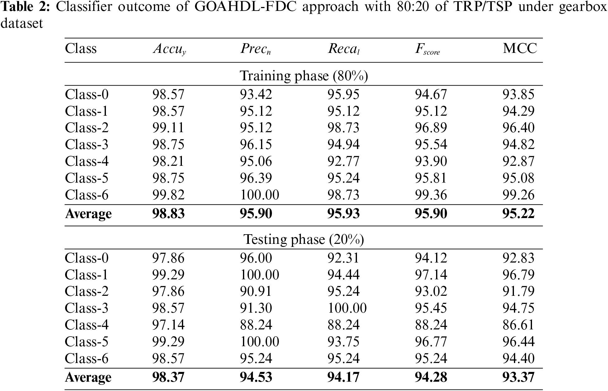
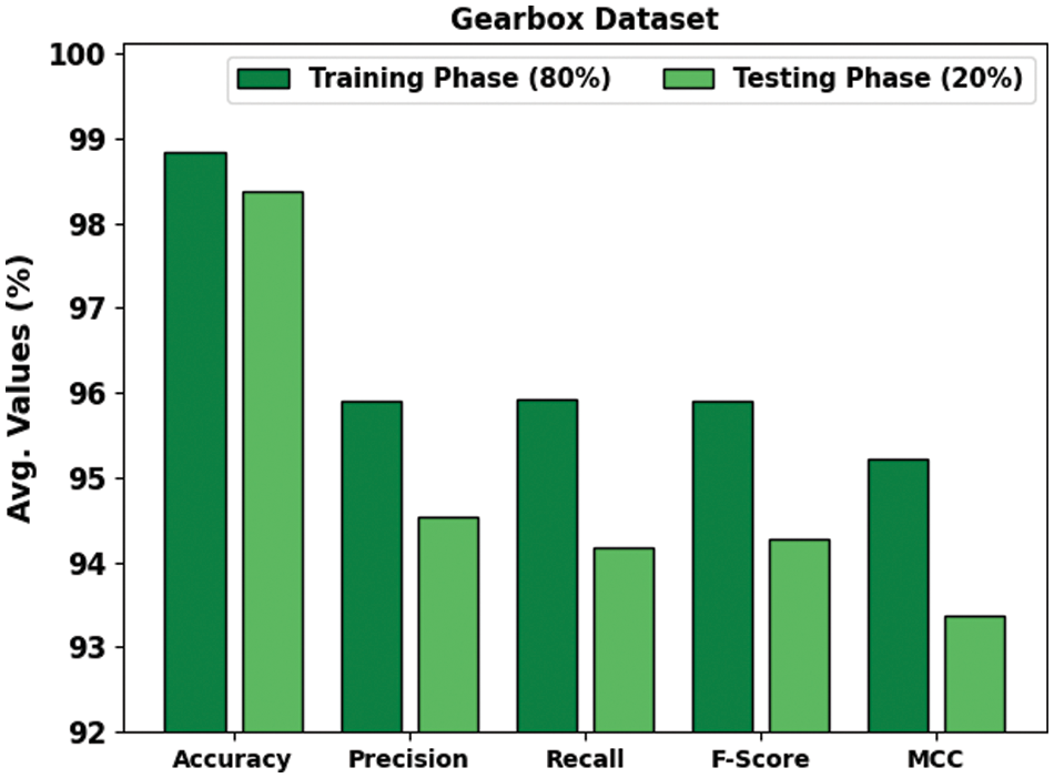
Figure 4: Average outcome of GOAHDL-FDC approach with 80:20 of TRP/TSP under gearbox dataset
A brief precision-recall (PR) curve of the GOAHDL-FDC technique is demonstrated on the Gearbox dataset in Fig. 5. The figure stated that the GOAHDL-FDC approach results in increasing values of PR. In addition, it is noticeable that the GOAHDL-FDC technique can reach higher PR values in all classes.
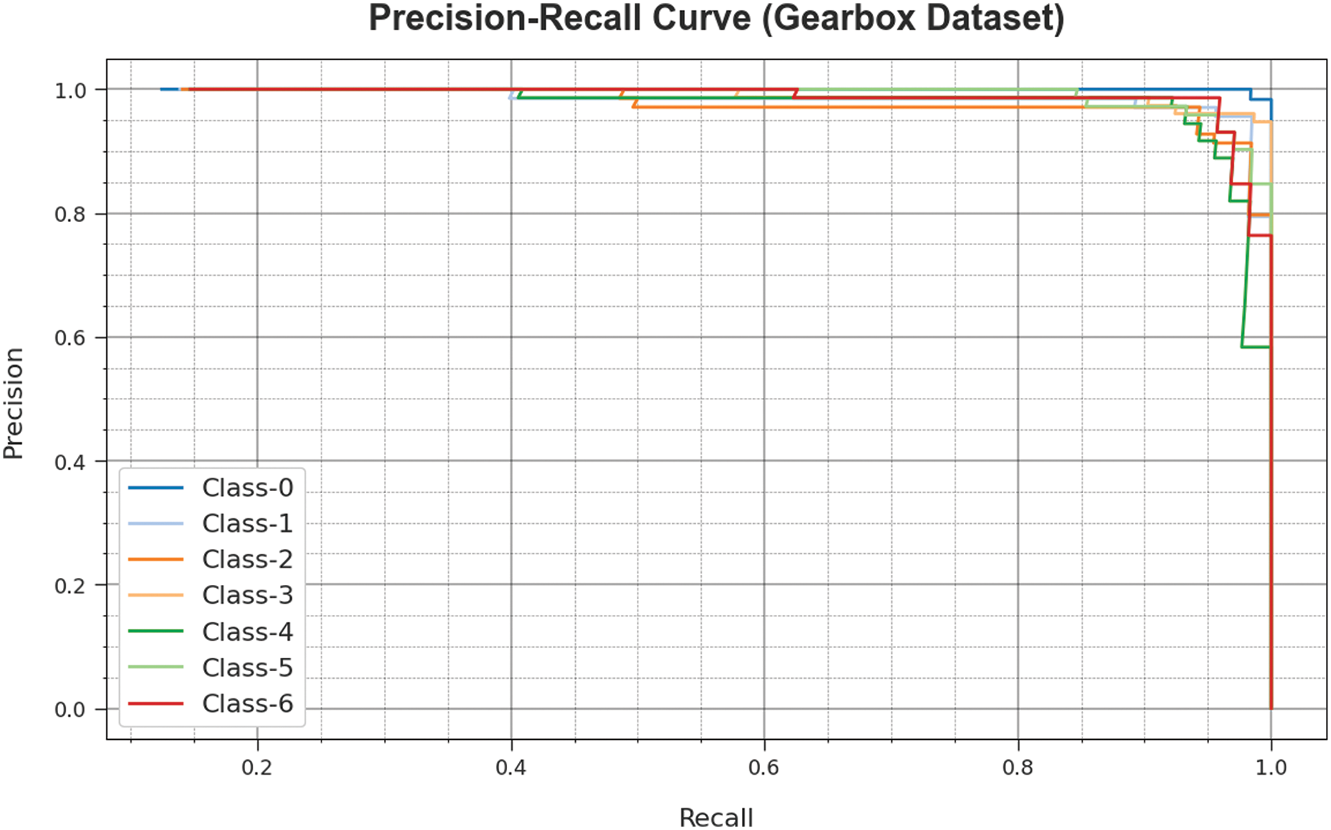
Figure 5: PR curve of GOAHDL-FDC approach under gearbox dataset
Fig. 6 inspects the accuracy of the GOAHDL-FDC approach during the training and validation process on Gearbox dataset. The figure specifies that the GOAHDL-FDC technique reaches increasing accuracy values over increasing epochs. As well, the increasing validation accuracy over training accuracy reveals that the GOAHDL-FDC technique learns efficiently on the Gearbox dataset.
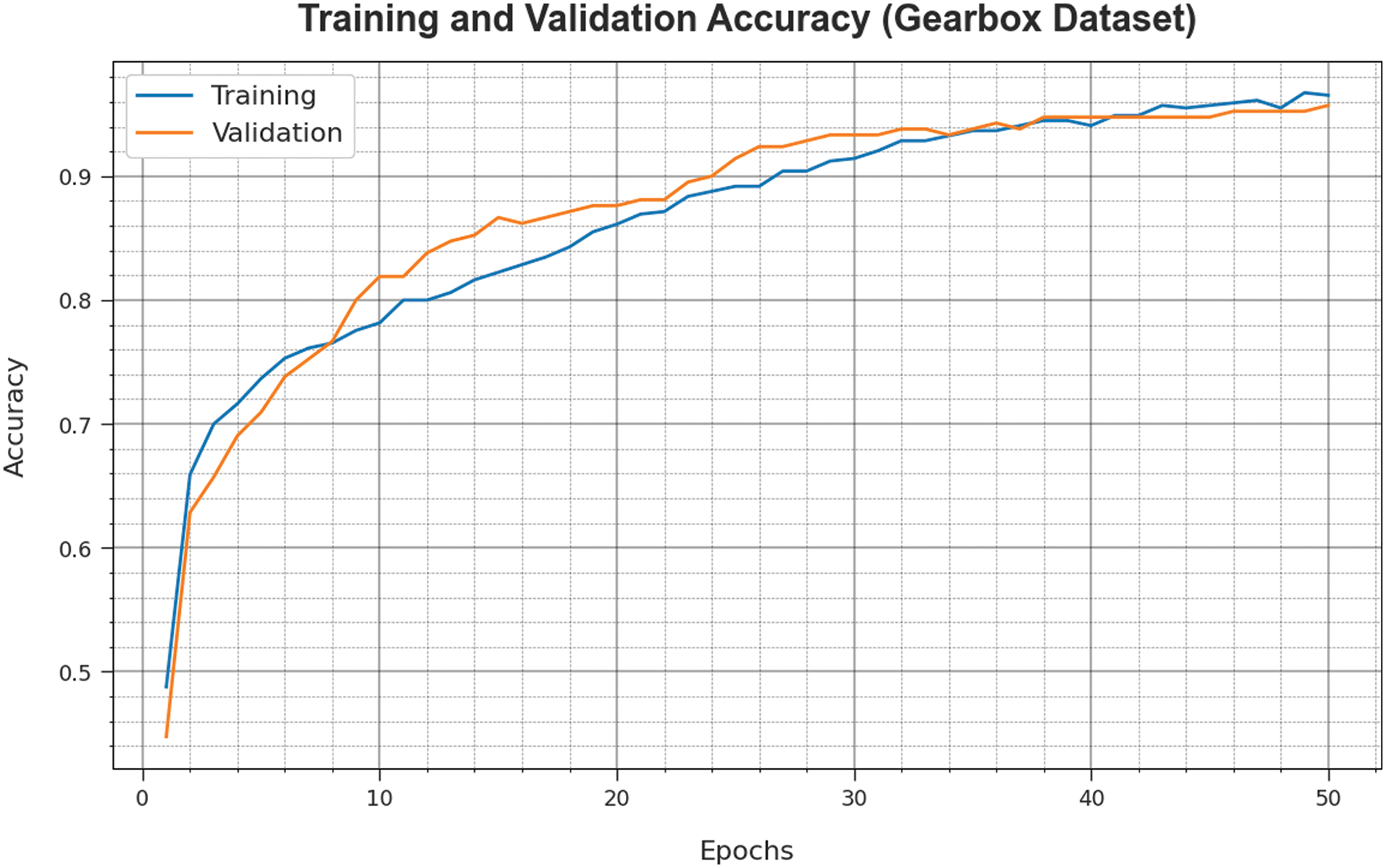
Figure 6: Accuracy curve of GOAHDL-FDC approach under gearbox dataset
The loss analysis of the GOAHDL-FDC method at the time of training and validation is given on the Gearbox dataset in Fig. 7. The outcomes indicate that the GOAHDL-FDC technique reaches closer values of training and validation loss. The GOAHDL-FDC approach learns efficiently on the Gearbox dataset.
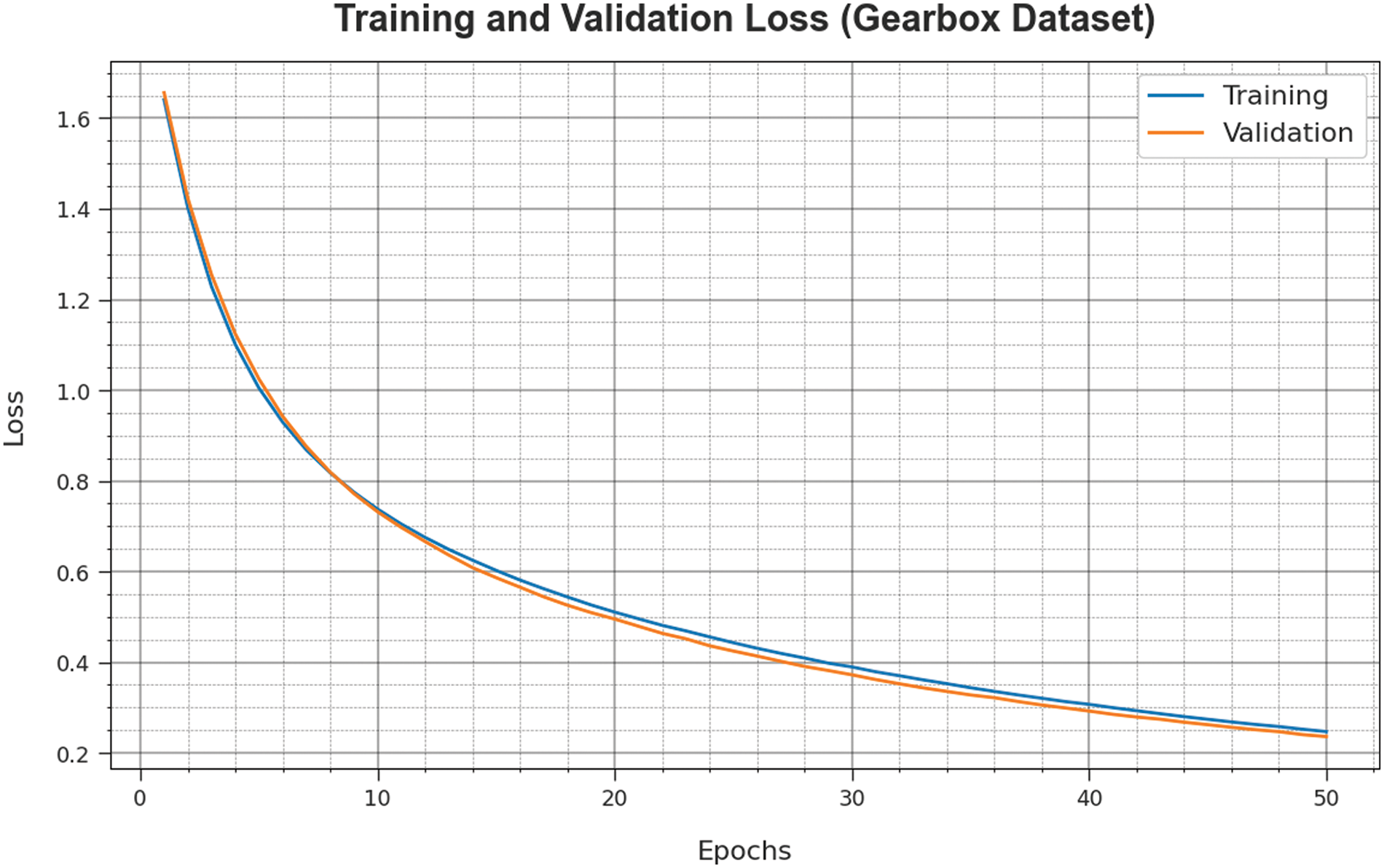
Figure 7: Loss curve of GOAHDL-FDC approach under gearbox dataset
In Table 3 and Fig. 8, the brief experimental results of the GOAHDL-FDC technique is studied under 70:30 of TRP/TSP of Bearing dataset. The average result analysis reported that the GOAHDL-FDC technique identifies all kinds of faults in the Bearing dataset. For instance, with 70% of TRP, the GOAHDL-FDC approach attains average
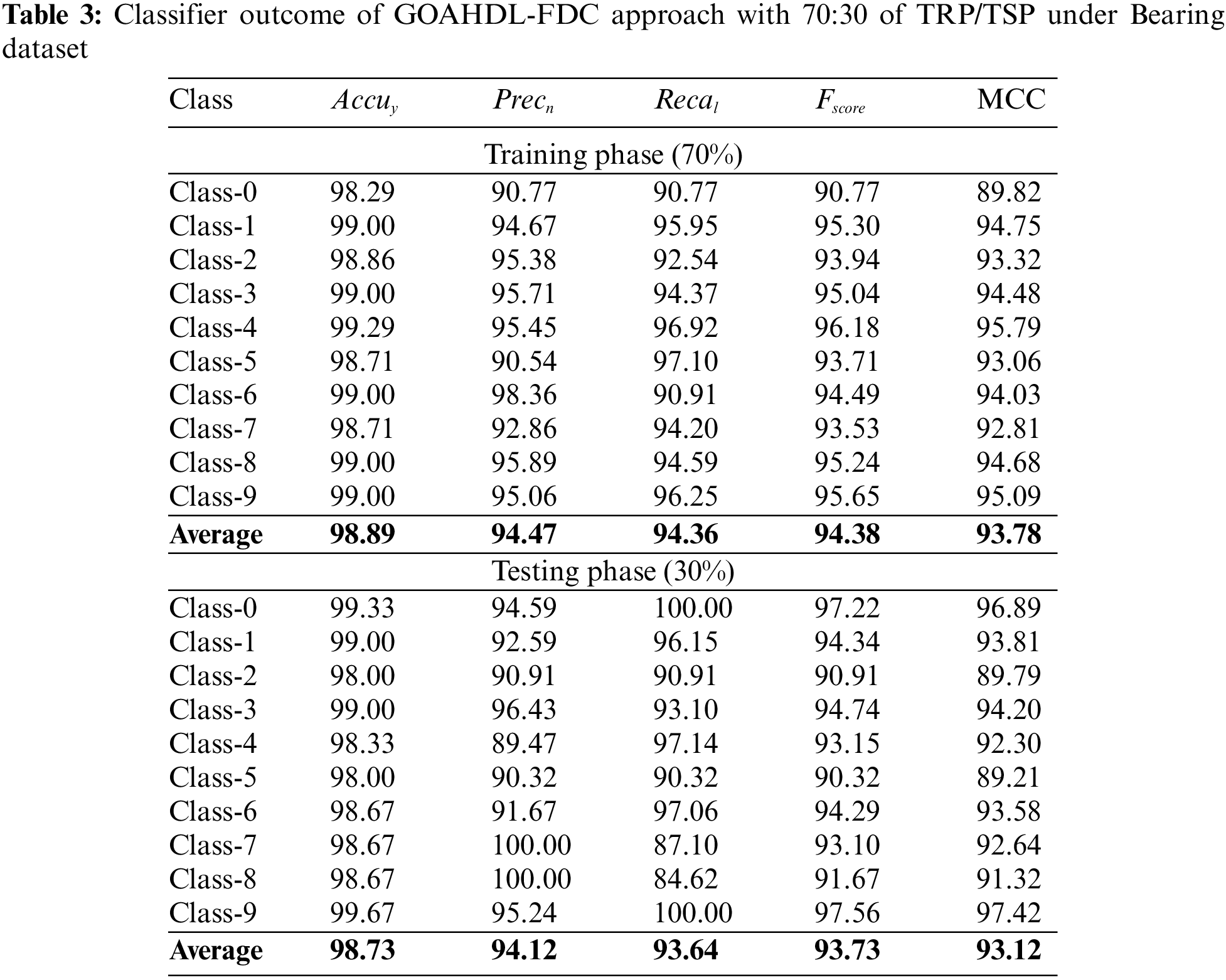
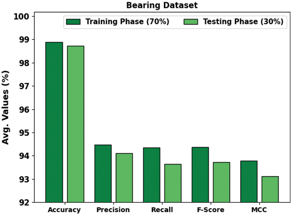
Figure 8: Average outcome of GOAHDL-FDC approach with 70:30 of TRP/TSP under Bearing dataset
In Table 4 and Fig. 9, the experimental results of the GOAHDL-FDC technique are studied under 80:20 of TRP/TSP of the Bearing dataset. The average result analysis reported that the GOAHDL-FDC technique identifies all kinds of faults in the Bearing dataset. For instance, with 80% of TRP, the GOAHDL-FDC technique attains average
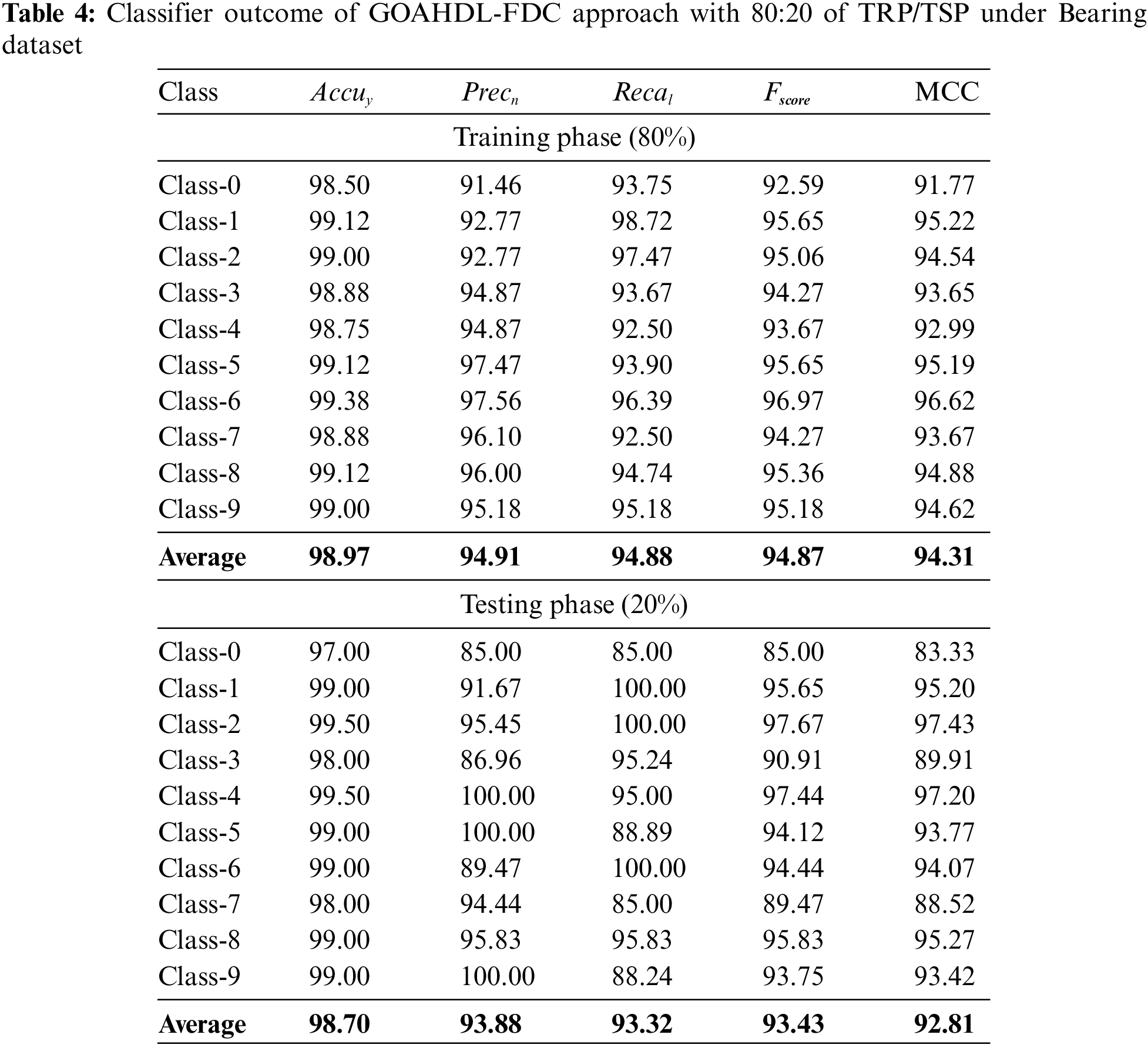
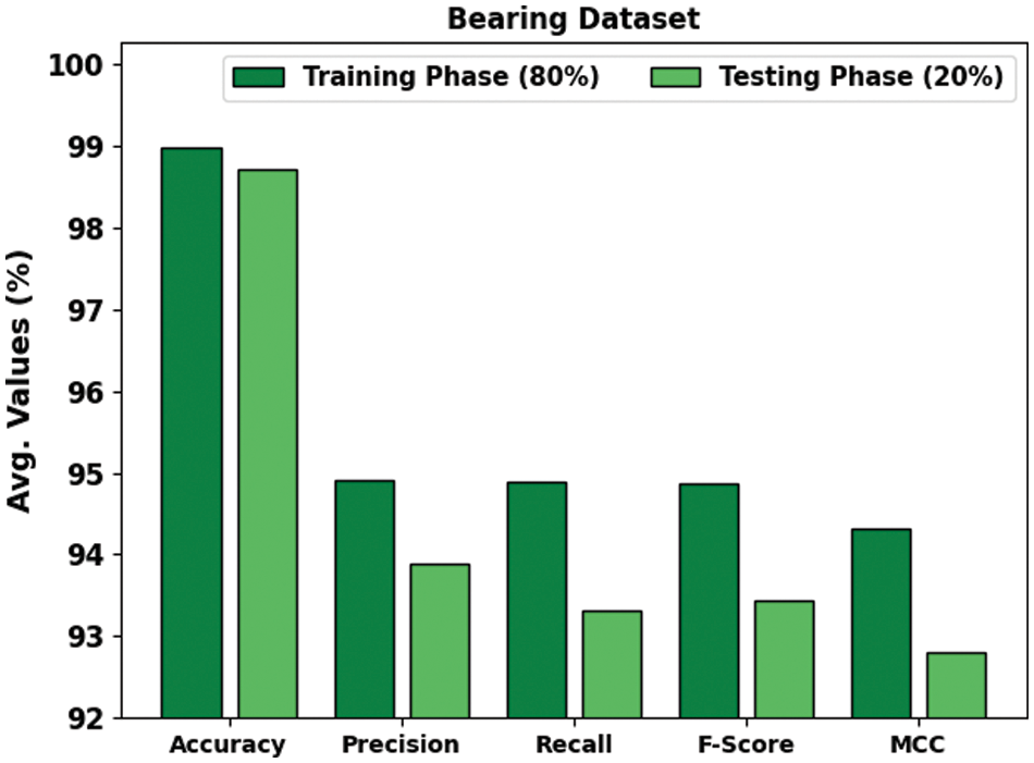
Figure 9: Average outcome of GOAHDL-FDC approach with 80:20 of TRP/TSP under Bearing dataset
A brief PR curve of the GOAHDL-FDC technique is illustrated on the Bearing dataset in Fig. 10. The figure states that the GOAHDL-FDC technique results in increasing values of PR. Also, it is noticeable that the GOAHDL-FDC approach can reach higher PR values in all classes.
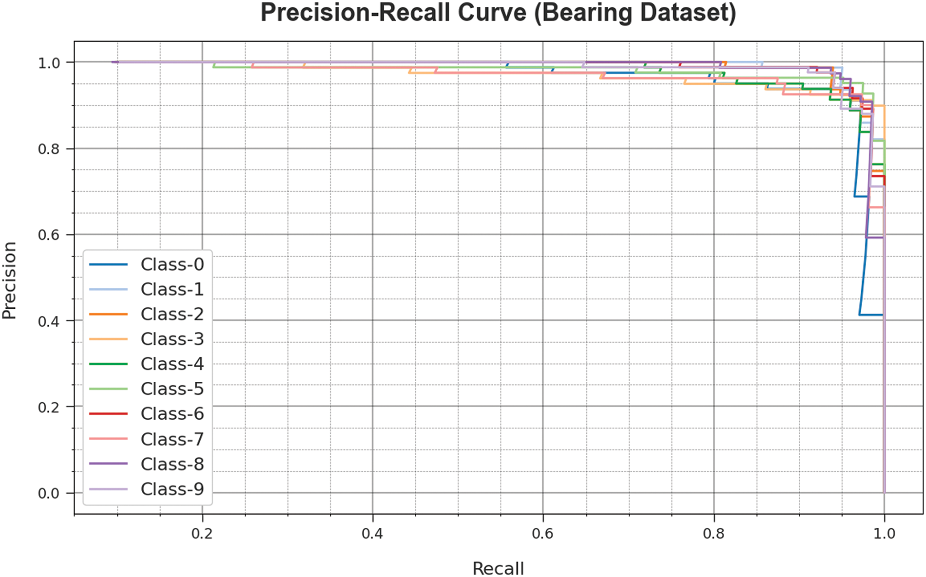
Figure 10: PR curve of GOAHDL-FDC approach under Bearing dataset
Fig. 11 illustrates the accuracy of the GOAHDL-FDC technique during the training and validation process on Bearing dataset. The figure states that the GOAHDL-FDC technique reaches increasing accuracy values over increasing epochs. In addition, the increasing validation accuracy over training accuracy displays that the GOAHDL-FDC approach learns efficiently on the Bearing dataset.
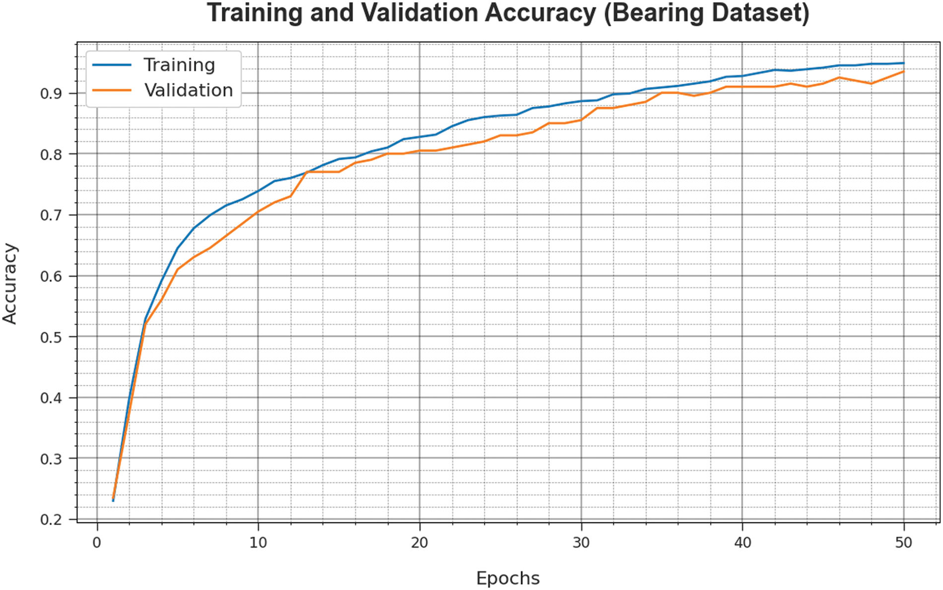
Figure 11: Accuracy curve of GOAHDL-FDC approach under Bearing dataset
The loss analysis of the GOAHDL-FDC approach at the time of training and validation is demonstrated on the Bearing dataset in Fig. 12. The figure indicate that the GOAHDL-FDC approach reaches closer values of training and validation loss. It is observed that the GOAHDL-FDC technique learns efficiently on the Bearing dataset.
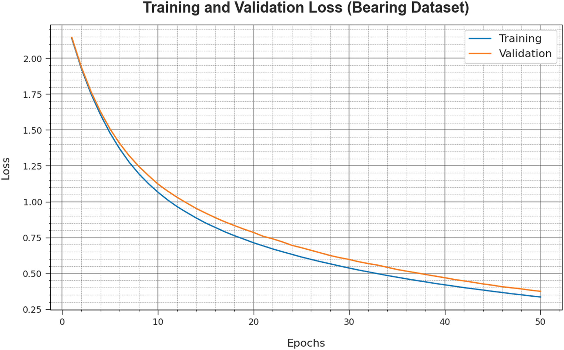
Figure 12: Loss curve of GOAHDL-FDC approach under Bearing dataset
To highlight the better performance of the GOAHDL-FDC method, a wide range of comparison studies is made in Table 5 [19]. Fig. 13 assesses the
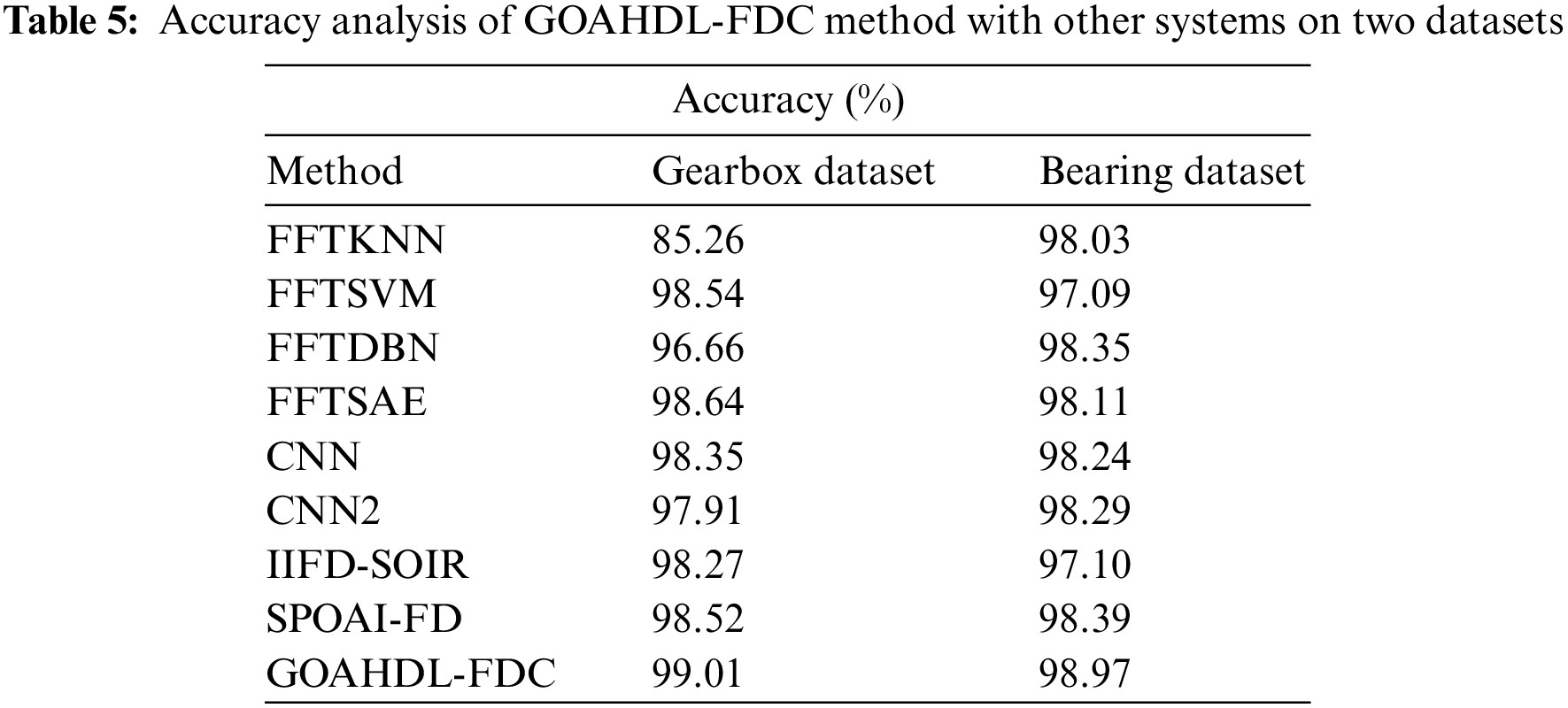
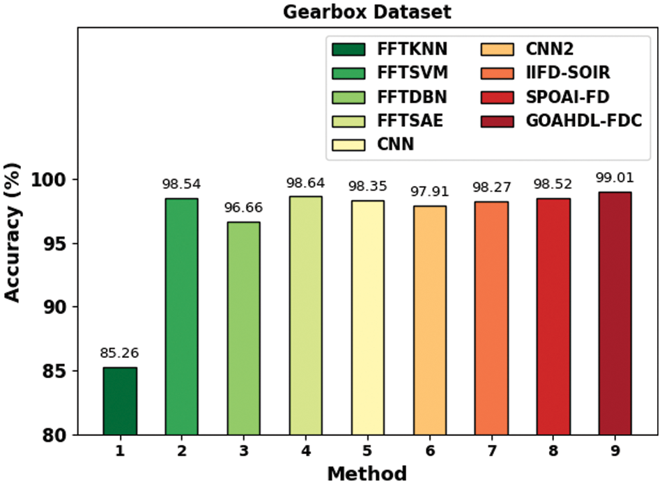
Figure 13: Accuracy analysis of GOAHDL-FDC approach under gearbox database
Fig. 14 assesses the
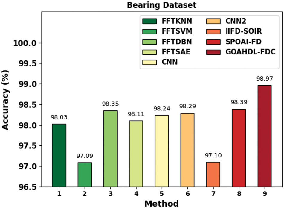
Figure 14: Accuracy analysis of GOAHDL-FDC approach under Bearing database
These results highlighted the superior characteristics of the GOAHDL-FDC technique in the failure detection process.
In this work, a novel approach is proposed that combines a gradient optimizer algorithm with hybrid deep learning techniques for failure detection and classification in the industrial environment. The proposed approach utilizes continuous wavelet transform (CWT) for preprocessing, a residual network (ResNet18) model for feature extraction, and the Gravitational Optimization Algorithm (GOA) for hyperparameter tuning of the Hybrid Deep Learning (HDL) model. The experimental results from simulations and experiments highlight the effectiveness of the proposed approach in improving fault diagnosis performance in various aspects. The proposed approach offers a promising paradigm for modern data-driven applications in the Industrial environment, providing a new direction for further research in the field of fault diagnosis in industrial systems.
In this article, we have focused on the design of the GOAHDL-FDC technique for accurate failure detection and classification in the industrial environment. The presented GOAHDL-FDC technique encompasses a series of operations such as CWT-based preprocessing, ResNet feature extraction, HDL-based failure detection, and GOA-based hyperparameter tuning. The presented GOAHDL-FDC technique primarily makes use of the CWT approach to preprocess the actual vibrational signals of the rotating machinery. Next, the ResNet18 model was utilized for the extraction of features from the vibration signals which are then fed into the HDL model for automated fault detection. Finally, the GOA-based hyperparameter tuning procedure is performed to adjust the parameter values of the HDL model accurately. The experimental validation of the GOAHDL-FDC approach is performed using a series of simulations and the experimentation outcomes highlight the better results of the GOAHDL-FDC technique under different aspects. In the future, the presented GOAHDL-FDC approach can be extended to the detection of intrusions in the industrial environment.
Acknowledgement: The authors would like to acknowledge the Deanship of Scientific Research (DSR) at King Abdulaziz University (KAU), Jeddah, Saudi Arabia.
Funding Statement: The Deanship of Scientific Research (DSR) at King Abdulaziz University (KAU), Jeddah, Saudi Arabia has funded this project under Grant No. (G: 651-135-1443).
Author Contributions: The authors confirm contribution to the paper as follows: study conception and design: M. Zarouan, I. M. Mehedi; data collection: S. A. Latif; analysis and interpretation of results: M. M. Rana; draft manuscript preparation: I. M. Mehedi. All authors reviewed the results and approved the final version of the manuscript.
Availability of Data and Materials: The data used to support the findings of this study are available in the manuscript.
Conflicts of Interest: The authors declare that they have no conflicts of interest to report regarding the present study.
References
1. Souza, R. M., Nascimento, E. G., Miranda, U. A., Silva, W. J., Lepikson, H. A. (2021). Deep learning for diagnosis and classification of faults in industrial rotating machinery. Computers & Industrial Engineering, 153, 107060. [Google Scholar]
2. Xue, Y., Dou, D., Yang, J. (2020). Multi-fault diagnosis of rotating machinery based on deep convolution neural network and support vector machine. Measurement, 156(2), 107571. [Google Scholar]
3. Cheng, Y., Lin, M., Wu, J., Zhu, H., Shao, X. (2021). Intelligent fault diagnosis of rotating machinery based on continuous wavelet transform-local binary convolutional neural network. Knowledge-Based Systems, 216(1), 106796. [Google Scholar]
4. Wu, C., Jiang, P., Ding, C., Feng, F., Chen, T. (2019). Intelligent fault diagnosis of rotating machinery based on one-dimensional convolutional neural network. Computers in Industry, 108(1), 53–61. [Google Scholar]
5. Liang, P., Deng, C., Wu, J., Yang, Z. (2020). Intelligent fault diagnosis of rotating machinery via wavelet transform, generative adversarial nets and convolutional neural network. Measurement, 159(4), 107768. [Google Scholar]
6. Choudhary, A., Mian, T., Fatima, S. (2021). Convolutional neural network based bearing fault diagnosis of rotating machine using thermal images. Measurement, 176(4), 109196. [Google Scholar]
7. Zhang, W., Li, X., Jia, X. D., Ma, H., Luo, Z. et al. (2020). Machinery fault diagnosis with imbalanced data using deep generative adversarial networks. Measurement, 152(3), 107377. [Google Scholar]
8. Yang, D., Karimi, H. R., Sun, K. (2021). Residual wide-kernel deep convolutional auto-encoder for intelligent rotating machinery fault diagnosis with limited samples. Neural Networks, 141(2), 133–144. [Google Scholar] [PubMed]
9. Zou, L., Li, Y., Xu, F. (2020). An adversarial denoising convolutional neural network for fault diagnosis of rotating machinery under noisy environment and limited sample size case. Neurocomputing, 407(3), 105–120. [Google Scholar]
10. Ma, S., Chu, F. (2019). Ensemble deep learning-based fault diagnosis of rotor bearing systems. Computers in Industry, 105(4), 143–152. [Google Scholar]
11. Zhao, X., Jia, M. (2019). A new local-global deep neural network and its application in rotating machinery fault diagnosis. Neurocomputing, 366(4), 215–233. [Google Scholar]
12. Li, X., Zhang, W., Ma, H., Luo, Z., Li, X. (2020). Domain generalization in rotating machinery fault diagnostics using deep neural networks. Neurocomputing, 403(1), 409–420. [Google Scholar]
13. Gong, W., Chen, H., Zhang, Z., Zhang, M., Wang, R. et al. (2019). A novel deep learning method for intelligent fault diagnosis of rotating machinery based on improved CNN-SVM and multichannel data fusion. Sensors, 19(7), 1693. [Google Scholar] [PubMed]
14. Zhang, Y., Zhou, T., Huang, X., Cao, L., Zhou, Q. (2021). Fault diagnosis of rotating machinery based on recurrent neural networks. Measurement, 171(3), 108774. [Google Scholar]
15. Li, Y. B., Du, X. Q., Wan, F. Y., Wang, X. Z., Yu, H. C. (2020). Rotating machinery fault diagnosis based on convolutional neural network and infrared thermal imaging. Chinese Journal of Aeronautics, 33(2), 427–438. [Google Scholar]
16. Surendran, R., Khalaf, O. I., Andres, C. (2022). Deep learning based intelligent industrial fault diagnosis model. Computers, Materials & Continua, 70(3), 6323–6338. https://doi.org/10.32604/cmc.2022.021716 [Google Scholar] [PubMed] [CrossRef]
17. Liu, X., Zhou, Q., Zhao, J., Shen, H., Xiong, X. (2019). Fault diagnosis of rotating machinery under noisy environment conditions based on a 1-D convolutional autoencoder and 1-D convolutional neural network. Sensors, 19(4), 972. [Google Scholar] [PubMed]
18. Li, H., Wang, T., Wu, G. (2022). A Bayesian deep learning approach for random vibration analysis of bridges subjected to vehicle dynamic interaction. Mechanical Systems and Signal Processing, 170, 108799. https://doi.org/10.1016/j.ymssp.2021.108799 [Google Scholar] [CrossRef]
19. Al Duhayyim, M., Mohamed, G., S.Alzahrani, H., Alabdan, J., Aziz, R. et al. (2022). Sandpiper optimization with a deep learning enabled fault diagnosis model for complex industrial systems. Electronics, 11(24), 4190. [Google Scholar]
20. Khalid, A., Iqbal, S., Abbas, S. (2022). Deep LSTM-BiGRU model for electricity load and price forecasting in smart grids (No. 8663). EasyChair. https://easychair.org/publications/preprint_open/NcTd [Google Scholar]
21. Altbawi, S. M. A., Mokhtar, A. S. B., Khalid, S. B. A., Husain, N., Yahya, A. et al. (2023). Optimal control of a single-stage modular PV-Grid-Driven system using a gradient optimization algorithm. Energies, 16(3), 1492. [Google Scholar]
22. Saravanakumar, R., Krishnaraj, N., Venkatraman, S., Sivakumar, B., Prasanna, S. et al. (2020). Hierarchical symbolic analysis and particle swarm optimization based fault diagnosis model for rotating machineries with deep neural networks. Measurement, 171(11), 108771. [Google Scholar]
23. Smith, W. A., Randall, R. B. (2015). Rolling element bearing diagnostics using the Case Western Reserve University data: A benchmark study. Mechanical Systems and Signal Process, 64, 100–131. [Google Scholar]
Cite This Article
 Copyright © 2024 The Author(s). Published by Tech Science Press.
This work is licensed under a Creative Commons Attribution 4.0 International License , which permits unrestricted use, distribution, and reproduction in any medium, provided the original work is properly cited.
 Downloads
 Citation Tools