A Novel Method for Determining Tourism Carrying Capacity in a Decision-Making Context Using q−Rung Orthopair Fuzzy Hypersoft Environment

1  Introduction

Making decisions can be daunting, particularly when we need more information and expertise in a specific area. However, we must not rely solely on our judgment but instead execute careful consideration and thoughtful analysis to make informed choices that result in favourable outcomes.

Different techniques have been used for decision-making problems, such as the application of RBF neural network optimal segmentation algorithm [1], stock intelligent investment strategy [2], smartphone app usage analysis [3], an algorithm for painting large objects [4], and multiscale feature extraction and multimodel fusion in visual question answering [5,6]. In 2022, Adak et al. [7] used a spherical distance measurement method for solving the MCDM problem under the Pythagorean fuzzy set. Debnath [8] used fuzzy hypersoft and developed a decision-making problem.

The idea of fuzzy logic was introduced by Zadeh [9,10], which involves the use of human experience to handle uncertain systems and assist decision-makers in making precise decisions [11,12]. Bellman and Zadeh proposed the concept of fuzzy sets [13]. Zadeh’s fuzzy set theory as a way to model uncertainty and imprecision in natural language, human reasoning, and complex systems. Since then, fuzzy set theory has been developed and extended in various directions, such as fuzzy logic, fuzzy relations, fuzzy measures, fuzzy analysis, possibility theory, type 2 fuzzy sets, etc. Fuzzy set theory has also found many applications in different disciplines, such as artificial intelligence, computer science, control engineering, decision theory, expert systems, logic, management sciences, operations research, robotics, and others [14].

However, the fuzzy set uses the degree of membership (MM) to describe the two states of support and opposition simultaneously. This may not be enough to grasp the uncertainty and imprecision in certain situations, where there may be a certain degree of hesitation or indeterminacy between support and opposition. To overcome this limitation, Atanassov [15] proposed an intuitionistic fuzzy set in 1983, an extension of a fuzzy set by adding a second index to measure the opposition state independently. In addition, a third index (i.e., degree of hesitation) can be derived from the degrees of MM and non-membership (N-MM) to quantify the state of indeterminacy. Since then, the intuitionistic fuzzy set theory has been developed and extended in various directions, such as interval values, type 2, neutrosophical, etc. Since then, the IFS idea has frequently been used to address real-world MCDM problems and challenges. IFS handles positive and negative membership grades only when the sum is less than or equal to 1. De et al. [16] created operations on intuitionistic fuzzy sets in 2002. Wang et al. [17] suggested several operations on IFS and created aggregation operators based on the fundamental operational laws. In addition, a multi-attribute decision-making (MADM) issue was created. Numerous studies [18,19] employed intuitionistic fuzzy sets in decision-making situations. The intuitionistic fuzzy set theory has also found many applications in different disciplines, such as artificial intelligence, computer science, control engineering, decision theory, expert systems, logic, management sciences, operations research, robotics, etc.

To overcome this limitation, Pythagorean fuzzy sets (PFS) were introduced by Yager et al. [20,21], which generalize IFS by ensuring that the square sum of MM and N-MM grades is equal to or less than 1. Several studies have developed different aggregation operators (AOs) in a Pythagorean fuzzy environment, distance measurement method and Pythagorean fuzzy power AOs [22,23].

In 2013, Cuong et al. [24] developed a picture fuzzy set. They assigned three degrees to each element of a universal set: a positive degree, a negative degree, and a neutral degree.

Hesitant fuzzy sets introduced by Torra [25] in 2010, hesitant fuzzy set assigns a set of possible degrees to each element of a universal set other than a single input.

Neutrosophic set initiated by Smarandache in 1998 [26], neutrosophic assigns three independent degrees to each element of a universal set, i.e., truth, indeterminacy, and falsity degree. The neutrosophic set can model the problem with a paradox or contradiction in the data, such as logic or philosophy.

Plithogenic set, also initiated by Smarandache in 2018 [27], are extensions of neutrosophic sets, where the truth, indeterminacy, and falsity degree are further refined into sub-degrees that shows different aspects of the data. For example, the truth degree can be divided into subjective, objective, and relative truth degrees.

However, fuzzy sets, intuitionistic fuzzy sets, and Pythagorean fuzzy sets have some limitations, such as the inability to handle indeterminacy, lack of flexibility, and generality to represent different types of uncertainty. To overcome these problems, Yager further generalized the concept of Pythagorean fuzzy sets by defining Rung orthpair fuzzy sets in 2017 [28], which used a parameter q to control the degree of orthogonality between the degrees of MM and N-MM. ROF sets are a special case of orthopair fuzzy sets, defined by two functions that satisfy certain orthogonality conditions. The ROFS can be reduced to intuitionist and Pythagorean fuzzy sets when q equals one and two, respectively. ROF sets can also capture different types of uncertainty by varying the q value. Since their inception, ROF sets have attracted a lot of attention from researchers and practitioners and have been applied to various fields, such as decision-making, data mining, raw sets, topology, logic, etc.

The theory of soft sets, introduced by Molodtsov [29] in 1999, is a mathematical tool for managing uncertainty and inaccuracy in various fields. A software set can handle situations where the membership of an element to a set depends on the choice of attributes. However, the theory of soft sets has certain limitations, such as the inability to handle situations in which attributes must be divided into disjoint sets of attribute values or when more than one set of attributes is involved. Cagman et al. [30] developed a fuzzy soft set and its application. In 2010, Majumdar et al. [31] proposed the structure of a generalized fuzzy soft set. Many researchers used the theme of fuzzy soft sets and developed some operations on it [32,33].

To overcome these limitations, Smarandache [34] extended the concept of the soft set by defining the hypersoft set theory in 2018. A hypersoft set is a pair of a multi-argument function and a discourse universe, where the function maps several sets of attributes to subsets of the universe. A hypersoft set can handle situations where the MM of an element to a set depends on the choice of several attributes and their values. Since their inception, flexible and hypersoftset theories have attracted a lot of attention from researchers and practitioners and have been applied to various fields of decision-making.

Background: Rung orthopair fuzzy hypersoft set is a hybrid of Rung orthopair fuzzy soft and hypersoft set, which is used to express insufficient and indefinite information in decision-making problems [35]. This is a way for the Rung orthopair fuzzy hypersoft set that uses multiparameter approximation functions to handle the shortcomings of all other versions of the fuzzy set. It can deal not only with the MMD of NMMD but also with the degree of hesitation and indeterminacy. It has been applied to various fields, such as selecting construction companies, thermal energy storage techniques, and multi-attribute group decision-making [36].

Research gap: ROFHS is a hybrid concept of orthopair Rung fuzzy soft set and hypersoft set, used to express insufficient and indefinite information in decision-making problems. ROFHS is a generalization of intuitionist fuzzy sets, Pythagorean fuzzy sets, and q−ROFS, representing the DMM, the NMMD, and the hesitant degree of an element for a set. One of the reasons for using ROFHS is that it can capture more information and uncertainties than other fuzzy set extensions, such as intuitionist fuzzy sets, Pythagorean fuzzy sets, or q−ROFS. The ROFHS can represent more orthopairs that satisfy the limits of the orthopair fuzzy sets with power and can also incorporate the parameters of the soft sets and the membership functions of the hypersoft sets. Therefore, ROFHS can provide a more complete and realistic way to model complex and dynamic situations. The concept of Rung orthopair fuzzy hypersoft sets was introduced by Khan et al. [37,38], which utilizes specific operational rules and aggregation operators (AOs) to address various interactions among input arguments. Subsequently, Gurmani et al. [39] proposed different AOs-based basic operational laws. However, there has been no investigation on Einstein AOs in the existing literature despite efforts on fuzzy and hypersoft sets with Rung orthopairs. This paper addresses this gap by proposing using geometric and average Einstein AOs and developing software that integrates these operators into decision-making processes. The management and capacity planning of tourist attractions could be a potential area of application for the Einstein AOs.

The structure of this paper is as follows: In Section 2, we conduct a literature review of prior studies. Section 3 covers the fundamental materials. We introduce operational laws and aggregation operators (AOs) that can assist in decision-making problems in Section 4. Section 5 presents an algorithm for the Multi-Attribute Decision Making (MADM) technique that illustrates expected AOs in decision-making. To demonstrate the effectiveness of the proposed technique, we present a numerical example to analyze the technique and note that the final result resembles q−ROFHSN. In Section 6, we provide a comparative study of the proposed framework and existing structures. Finally, Section 7 concludes the paper by summarizing the results and highlighting future research directions.

1.1 Related Work

The tourist carrying capacity refers to the large number of visitors that a destination can accommodate sustainably without causing a negative impact on the environment, quality of residents, and culture. Some policymakers suggest balancing the development of tourism with the preservation of resources. Recently, Qiao et al. [40] studied embodiment theory and sensory compensation theory to examine the aspect of the tourism experience perspective of visually impaired tourists. Many researchers studied tourism with different perspectives, such as assessing quality tourism [41], tourism carrying capacity, a fuzzy approach [42], and economic and environmental impact of the tourism carrying capacity [43]. Many researchers worked on different decision-making approaches, such as deducting sudden rainstorm scenarios by decision-making [44] and an abstract syntax-based static fuzzing mutation for vulnerability evolution analysis [45]. Yuan et al. [46] in 2022 developed the system dynamic approach for evaluating the interconnection performance of cross-border transport. One of the applications of fuzzy sets and fuzzy logic in this estimation is the fuzzy linear programming model proposed by Fernández-Villarán et al. [47]. They developed a model to measure the TCC of an inhabited tourist destination (such as a country, region, or municipality), thanks to alerts that can help destination managers take action. The model considers the four dimensions of CBT: physical-ecological, social-demographic, economic, and perceptual. Each dimension has several indicators measured by vague numbers, representing the degree of satisfaction or dissatisfaction of tourists and residents with each indicator. Another example of using fuzzy sets and fuzzy logic to estimate CBT is the fuzzy set load capacity model (FTCC) proposed by Bertocchi et al. [48]. They focused on the case of Venice, one of the world’s most representative cases of over-tourism. Their objective is to determine a sustainable scenario for the number of tourists in Venice by looking for the best compromise between the local tourist sector’s monetary gains and the local population’s harmful effects on the destination. The model considers three types of tourists: tourists who sleep in hotels, tourists who sleep in other forms of accommodation, and day trips. Each type of tourist impacts the destination differently in terms of expenses, congestion, pollution, waste production, etc.

2  Materials and Methods

In this section, we gather some fundamental data that will be used to construct the outline of the article.

Definition 2.1. [35] The mathematical form of a Rung orthopair fuzzy hypersoft set (q−ROPHS set) over a universe of discourse X can be defined as:

where represents the family of all possible subsets of q−ROF X, where and are the MM and N-MM with condition

For simplicity, are denoted as is represents a ROFHN.

Definition 2.2. [36] The Rung orthopair fuzzy hypersoft weighted average (q−ROFHWA) operator is a generalization of the traditional weighted average operator that considers the input information’s uncertainties and vagueness. The mathematical form of the q−ROFHWA operator can be expressed as follows:

(1)

where and are weight vectors with the condition and And their mapping is defined as .

Definition 2.3. [36] The Rung orthopair fuzzy hypersoft weighted geometric (q−ROFHWG) operator is a generalization of the traditional weighted geometric operator that considers the uncertainties and vagueness of the input information. The mathematical form of the q−ROFHWG operator can be expressed as follows:

(2)

where and are weight vectors with the condition, and And their mapping is defined as .

Definition 2.4. [37] The score function of the ROFHNs is defined as

3  Use of Einstein Operations in the Context of ROFHNs

Einstein t-norms and t-conorms are constructed by using specific fixed values. Einstein operations refer to arithmetic operations employed to manipulate fuzzy sets. The Einstein operations for ROFHNs are presented below:

Definition 3.1. The Einstein product and Einstein sum are two fuzzy arithmetic operations commonly employed in fuzzy logic and fuzzy set theory. They represent t-norm and t-conorm, respectively, and are defined as follows:

(3)

(4)

Our research now investigates Einstein’s operational laws, which can be described as follows:

Definition 3.2. For any two ROFHNs and with n > 2,

1.   

2.   

3.   

4.   

Theorem 3.1. For any two ROFHNs and with any

1.   

2.   

3.   

4.   

5.   

6.   

3.1 Einstein Aggregation Operators

In this section, we will develop ROFHS Einstein weighted average (q−ROFHEWA), weighted geometric (q−ROFHEWG), ordered weighted average (q−ROFHEOWA), and ordered weighted geometric (q−ROFHEOWG) aggregation operators by using Einstein basic laws. These operators are then typically defined to overcome their ROFHN aggregation errors. The Einstein weighted average operator is a powerful tool for handling uncertainty and imprecision in data analysis and decision-making. It has many applications in areas such as finance, engineering, environmental science, and artificial intelligence, where decision-makers must combine multiple sources of uncertain information to reach a consensus or make a decision.

Definition 3.3. Let be a ROFHNs, w, and v represents experts and attributes weights, respectively, with the condition We define the q−ROFHEWA operator as follows:

(5)

Theorem 3.2. Let \ \ be \ROFHNs, with the weight of experts W\ and attributes V\ with \ Then, the aggregated result of the q−ROFHEWA operator is always \ROFHN obtained by the following equation:

(6)

Proof. We will demonstrate the proof of this theorem using the mathematical induction method.

1.   When it follows that and thus the left-hand side of Eq. (5) can be expressed as follows:

For the right side of Eq. (6) we have

Consider the case where . In this scenario, the following applies:

Therefore, Eq. (6) holds for the values of and

3.   Assuming that Eq. (6) is valid for , we obtain the following expression:

So the result is true for and , and therefore true for all values of .

The following theorem describes some fundamental properties of the proposed q−ROFHEWA operator.

Theorem 3.3. The q−ROFHEWA operator has the following properties:

1.   (Idempotency) If all are equal, i.e., for all v and w, then

2.   (Boundedness) Let be a family of and let then

3.   (Monotonicity) Let and be two sey = ts of if for all v and w, then

Proof. (1) For by 3.5, the result is yielded below:

(2) There exist the inequality when and Thus, there also exists Then the inequality can be kept regarding the above properity (1), there is

(3) For there is the inequality i.e., exists. Therefore, all the above properties are true.

Further, we explain the q−ROFHEWG operator as follows:

Definition 3.4. Let be a ROFHNs, w, and v represent the weight with the condition Then, the q−ROFHEWG operator is represented as:

Theorem 3.4. Let \ \ be \ROFHNs, with the weight of experts \ and attributes \ for \ Then the aggregated result of the q−ROFHEWG operator is again \ROFHN obtained by the following equation:

(7)

Proof. Same as the above theorem.

Theorem 3.5. The q−ROFHEWG operator implies the following properties:

1.   Idempotency: If all are equal, i.e., v and w, then

2.   Boundedness: Let be a family of and let then

3.   (Monotonicity) Let and be two sets of if for all v and w, then

Proof. Proof straight forward.

Definition 3.5. Let be a ROFHNs, w, and v represents experts and attributes weights, respectively, with the condition We define the q−ROFHEOWA operator as follows:

Here r, s are permutations such that and , .

Theorem 3.6. Let \ \ be \ROFHNs, with the weight of experts W\ and attributes V\ with \ Also r, s are permutations such that \ and \, \. Then, the aggregated result of the q−ROFHEOWA operator is always \ROFHN obtained by the following equation:

(8)

Proof. We will demonstrate the proof of this theorem using the mathematical induction method.

1.   When , it follows that and thus the left-hand side of Eq. (8) can be expressed as follows:

By using Eq. (8), we get the following:

Consider the case where . In this scenario, the following applies:

Therefore, Eq. (9) holds for the values of and

3.   Assuming that Eq. (9) is valid for , we obtain the following expression:

So the result is true for and , and therefore true for all values of .

The following theorem describes some fundamental properties of the proposed q−ROFHEOWA operator.

Theorem 3.7. The q−ROFHEOWA operator has the following properties:

1.   (Idempotency) If all are equal, i.e., for all v and w, then

2.   (Boundedness) Let be a family of and let then

3.   (Monotonicity) Let and be two sey=ts of if for all v and w, then

Proof. (1) For by 3.5, the result is yielded below:

(2) There exist the inequality when and Thus, there also exists Then the inequality can be kept regarding the above properity (1), there is

(3) For there is the inequality i.e., exists. Therefore, all the above properties are true.

Further, we explain the q−ROFHEWG operator as follows:

Definition 3.6. Let be a ROFHNs, w, and v represent the weight with the condition Then, the q−ROFHEOWG operator is represented as:

Theorem 3.8. Let \ \ be \ROFHNs, with the weight of experts \ and attributes \ for \ Then the aggregated result of the q−ROFHEOWG operator is again \ROFHN obtained by the following equation:

(9)

Proof. Same as the above theorem.

We show some fundamental properties of the q−ROFHEOWG operator in the following theorem:

Theorem 3.9. The q−ROFHEOWG operator implies the following properties:

1.   Idempotency: If all are equal i.e., v and w, then

2.   Boundedness: Let be a family of and let then

3.   (Monotonicity) Let and be two sets of if for all v and w, then

Proof. Proof straight forward.

4  Multi-Attribute Decision-Making (MADM) Approach in the Context of ROFHNs

MADM is an approach that evaluates different alternatives by considering multiple criteria or attributes simultaneously. MADM has broad applications in engineering, management, finance, and environmental science. Researchers have recently shown a growing interest in using FSs, particularly ROFHS, in MADM. In the MADM approach under ROFHS, the evaluation criteria or attributes are represented using ROFHS. The alternatives are evaluated based on each criterion, and the results are combined to evaluate each alternative. Several methods can be used to combine the results of the evaluations, including the weighted average weighted geometric mean. Using q−ROFHSs in MADM has several benefits over traditional approaches. Firstly, it provides a more flexible representation of uncertainty, which can lead to more precise and reliable decision-making. Secondly, it allows for a more intuitive representation of decision-maker’s preferences, which can help improve the decision-making process’s transparency and acceptability. Finally, this approach effectively tackles complicated decision-making challenges with multiple criteria and alternatives. Considere to be a set of alternatives and be a set of experts. The weights of experts are given as and Let be a set of attrbutes. Furthermore, this approach can be applied to handle corresponding multi-subattributes, such as s with weights such as Components of the collection sub-attributes have multiple values; For simplicity, the components of can be specified as Expert group reviews alternatives under the preferred sub-attributes of considered parameter has the form of ROFHN such that . Now, using the proposed weighted AOs, we evolve the algorithm to solve the MADM problem in the q−ROFH environment. Fig. 1 illustrates a commonly used format for the MADM methodology. The structure shown in this figure typically involves the identification of criteria, assessment of alternatives against criteria, the use of aggregation operators and selection of optimal alternative. Because for this purpose, we develop the following algorithm:

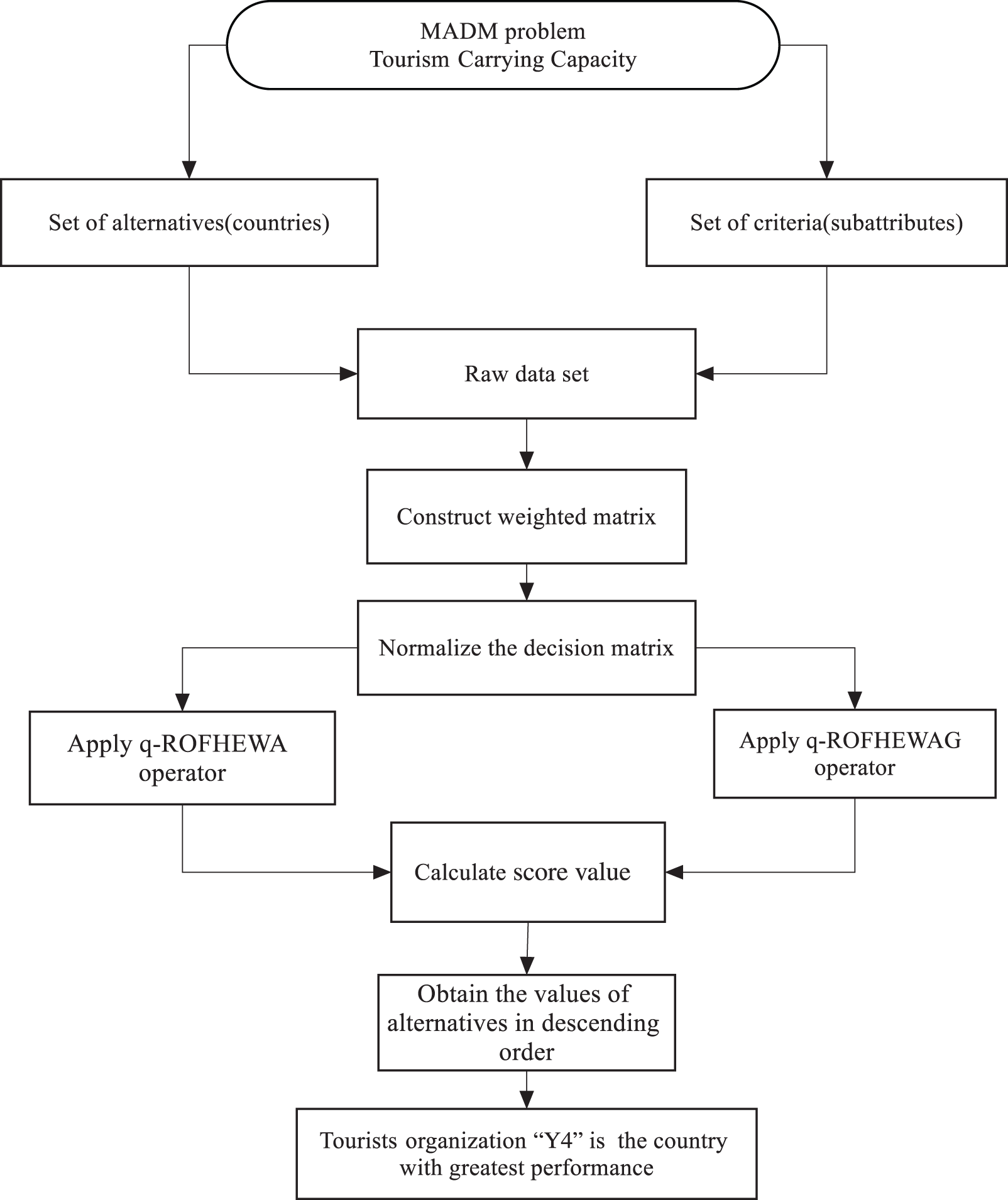
Figure 1: Proposed method

4.1 Decision Making

Decision-making is very important in real life. So, we need to make a decision in most real-life problems, such as economy, technology, politics, and management. In the economy, we know that decisions have a major impact on customer cost, manufacturing, service, and efficiency. The same is true for tourists carrying capacity. It is the best result for tourist companies to choose the best tourist location. For a tourist’s location, it is important to select the best tourist location for the tourists. According to the World Tourism Organization (WTO), the term “tourism carrying capacity” refers to the highest number of visitors that can visit a tourist destination simultaneously, without causing any harm to the natural, economic, cultural, social, and environmental aspects of the destination, as well as without causing any unacceptable degradation in the quality of visitor enjoyment. So, for this purpose, we want to increase tourism, a tourism organization wishes to evaluate a tourism carrying capacity with qrung orthopair fuzzy hypersoft information. By collecting all possible information about tourism carrying capacity, the expert group selects five different countries India, Nepal, China, Pakistan, and Bangladesh, i.e., represented by The expert group select a set of attributes as E = Social environmental carrying capacity, Limit of acceptable change, Visitors experience and resource protection. Let the corresponding sub-attributes are:

e = { = food availability, = water, = space

e = { = specification of achievable resources, = identification of management action

e = { = Education and community goal, = demographic and learning motivation

Let É = {e × e × e} be a set of subattributes

É = {} {A} {A}

= {} {} {} {} {} {}

Set of multi-subattributes with weights is Let the set of three experts be define as with weights to udge the optimim alternatives. The overall rating of the alternative should be used to make a decision. This can be expressed in fuzzy numbers using the expression ROFHNs. Specialists provide their preferences in the form of ROFHNs, which are used to determine the best alternative among a set of options using Multi-Attribute Decision Making (MADM) techniques. Finally, the relative closeness of each alternative to the ideal solution is determined, and the alternatives are ranked accordingly.

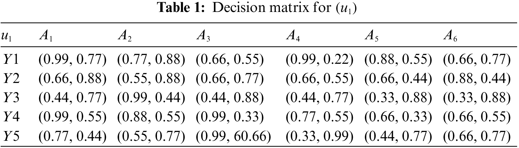
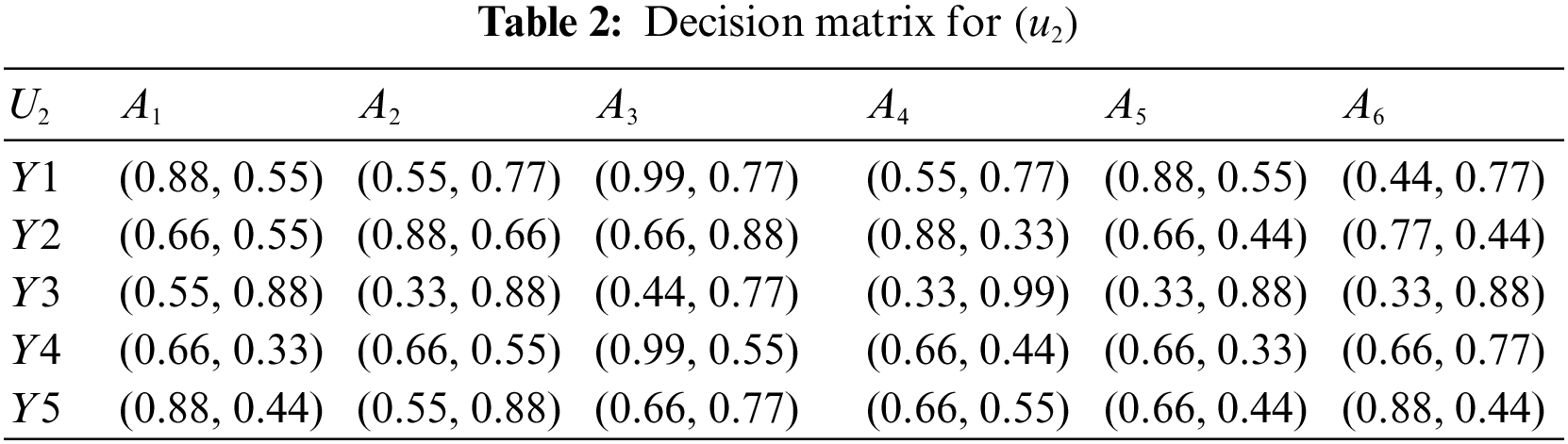
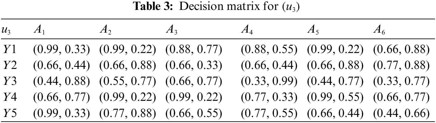
Step 1. Tables 1 to 3 summarise the experts’ priorities in the form of ROFHNs.

Step 2. If all attributes are of the same type, then there is no need for normalization.

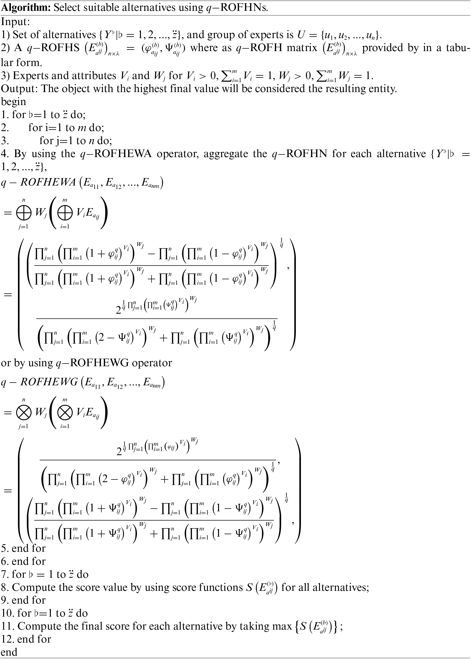
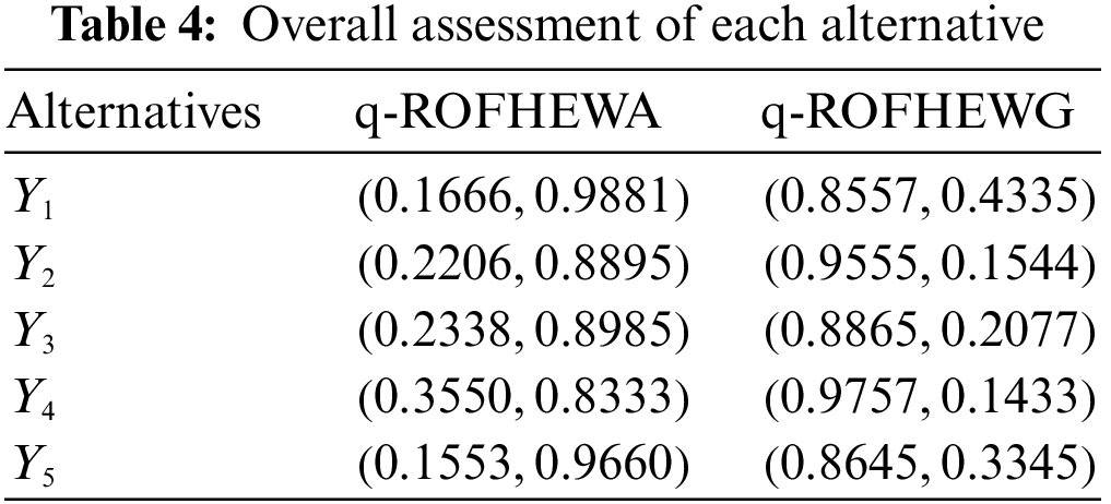
Step 3. Integrate the attribute information for each tourism carrying capacity by assuming that q = 3, using either the q−ROFHEWA or q−ROFHEWAG operator, The resulting data is displayed in Table 4.

Step 4. Calculate the score values for each alternative.

Step 5. Based on the scoring feature, rank the pros and cons of tourist transportation capacity. For the q−ROFHEWA operator, the value of the score function is:

As can be seen, the tourist organization with the greatest overall performance is . Fig. 2 shows a visual representation of the score values.

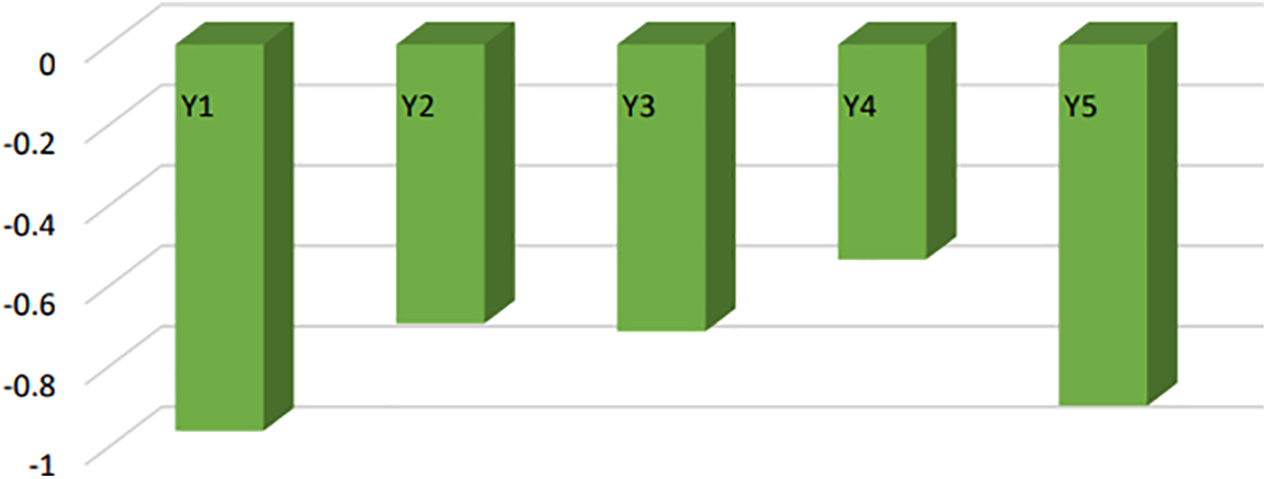
Figure 2: Ranking result of alternatives

5  Comparative Study

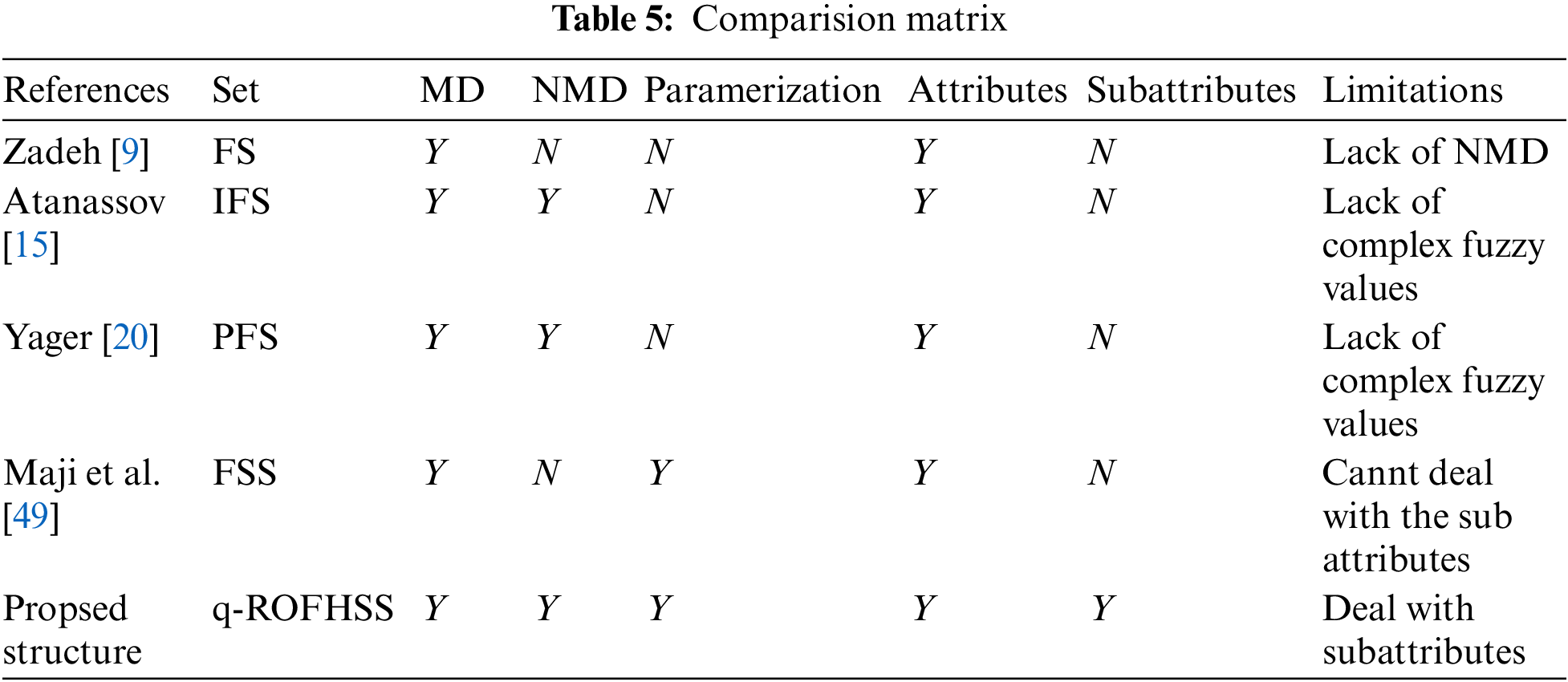
In this section, we assess the proposed method from the point of view of its efficiency, operability, simplicity, and benefits and compare it to some existing structures. Zadeh’s FS [9] provided decision-makers with information to solve uncertain problems by considering only the MMD. Currently, FS uses MMD information to solve difficulties in decision-making problems, while our proposed structure utilizes the inherent ambiguity in both MMD and N-MMD cases. Atanassov [15] presented the MM and N-MMD in their intuitionistic fuzzy sets. However, in some decision-making situations, the sum of MM and N-MMD may exceed 1. Yager [20] used MMD and N-MMD to deal with uncertainty in their PFS by expanding IFS. The theory of Soft sets [49] was introduced to tackle the challenge of parameterizing uncertain and ambiguous data. The soft set theory accounts for the complexity of decision-making problems in real-world scenarios compared to other uncertain theories. Fuzzy soft sets were subsequently developed to address the uncertainty issues. However, this structure does not provide information about N-MMD. To overcome this limitation, Maji [50] proposed the concept of intuitionistic fuzzy soft sets. Intuitionistic fuzzy sets cannot handle situations where the sum of MM and N-MM exceeds 1. However, the ROFHS structure we propose can overcome this limitation in the context of fuzzy hypersoft sets, which other structures cannot. ROFHS is a special case of FS and IFS that meets certain requirements. None of the previously mentioned structures offer information about sub-attributes. To address this issue and to provide more useful outcomes to the MADM problem, our proposed structure covers these limitations. Accurately and empirically representing feature information can significantly enhance the effectiveness of the MADM problem, as shown in Table 5. Based on the study’s results and comparisons, it was determined that the proposed technique outperforms existing methods in DM problems. Given that the proposed model is more efficient, flexible, competent, and adaptable than other hybrid structures of fuzzy sets, it can continue to work hard despite disturbances that may occur. The results obtained from the proposed techniques are different from the hybrid techniques, and the operator of the proposed structure is more capable, dependable, and efficient.

5.1 Impact of Parameter q on the Decision Result

This section addresses the effect of the parameter q on the ranking result. To look at the effect of different values of and in this case. The aggregated score values and the corresponding ranking results correspond to and operators are presented in Tables 6 and 7. From these tables, it seems that different point values are obtained from different values of parameter q, and the final classification result remains the same for each case. Next, we analyzed how the different parameters affected the results of the alternatives. We found that the value of the score function of the q−ROFHEWA operator changes gradually as the q parameter increases. In contrast, the value of the score function of the q−ROFHEWG operator decreases progressively with an increase in the q parameter. However, these changes do not affect the outcome of the alternative, which remains the same as before. A graphical representation of different q values for the WA operator can be plotted with the x-axis representing q values and the y-axis representing the corresponding values of the score function. As q increases from 0 to 1, the value of the score function of the WA operator increases monotonically. However, as q increases from 1 to infinity, the score function value of the WA operation decreases monotonically. At q = 1, the score function value of the WA operator is equal to the arithmetic mean of the input values, which is a special case of the WA operator. The plot demonstrates that the choice of q value can influence the score function values of the WA operator. Figs. 3 and 4 represent a visual representation of the data presented in Tables 6 and 7.

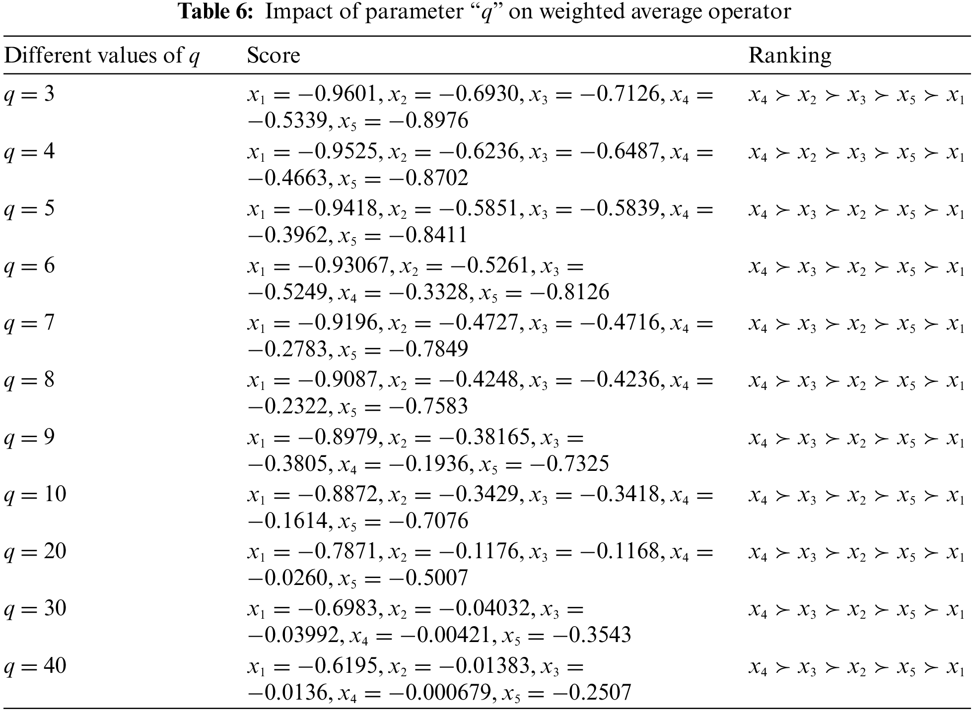
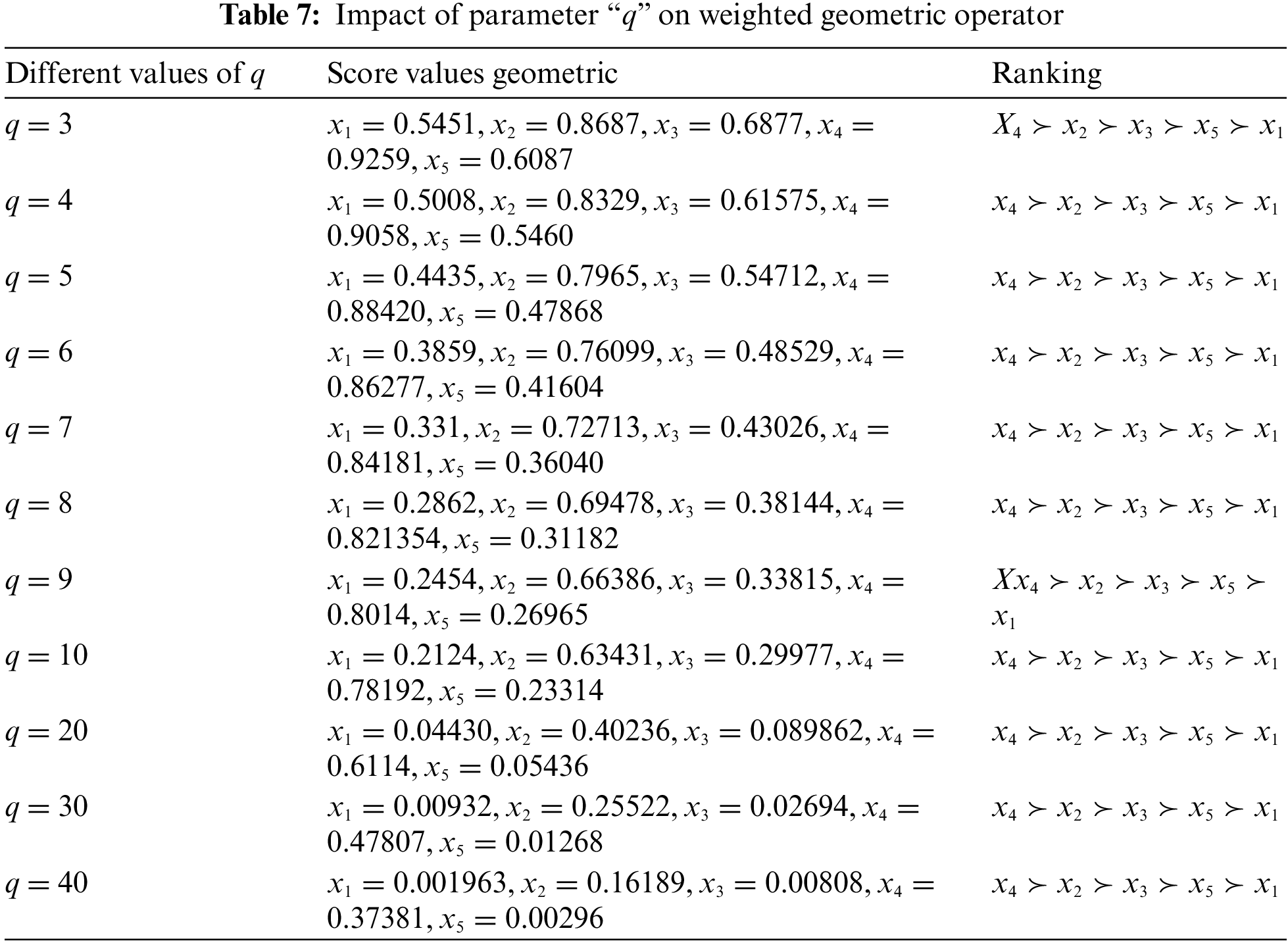
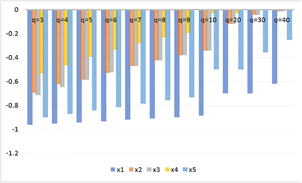
Figure 3: Graphical representation of different values of “q” for weighted average operator

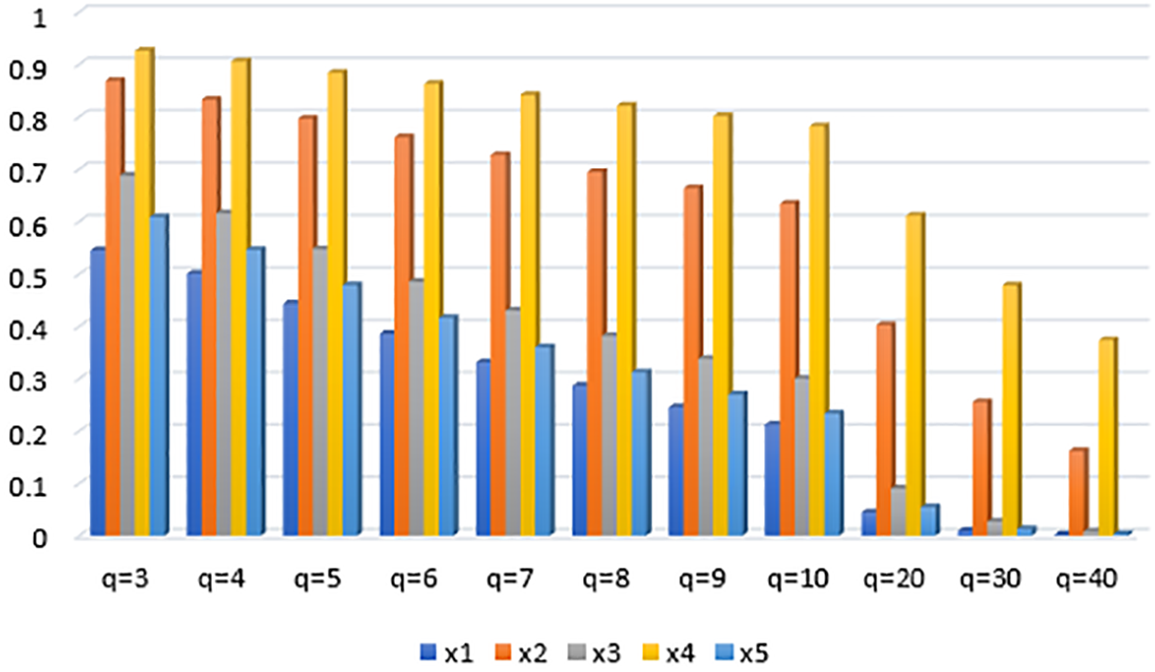
Figure 4: Graphical representation of different values of “q” for weighted geometric operator

5.2 Comparision with Existing Method

This section will compare our findings to those of certain existing operators. Zulqarnain et al. [51] proposed Pythagorean fuzzy soft (PFS) operators and discussed their features. However, these operators only deal with parameterized values of the alternative’s attributes and cannot handle multiple subattributes of the considered parameters. Zulqarnain [52] also proposed interaction operators for PFSs, but they have the same limitation. The IFHWA and IFHWG [53] operators can handle multiple subattributes, but they cannot be used when the sum of the MMD and N-MMD of the various subattributes reaches one. In contrast, our proposed q−ROFHEWA and q−ROFHEWG operators can overcome these limitations, making them more robust for solving MADM problems. Therefore, we believe that our proposed operators can improve the effectiveness of the DM technique in the future.

A comparison of the ranking results is presented in Table 8. Fig. 5 illustrates the ranking of alternatives, alongside several existing approaches.

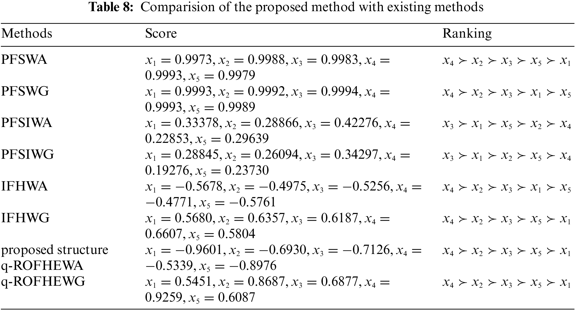
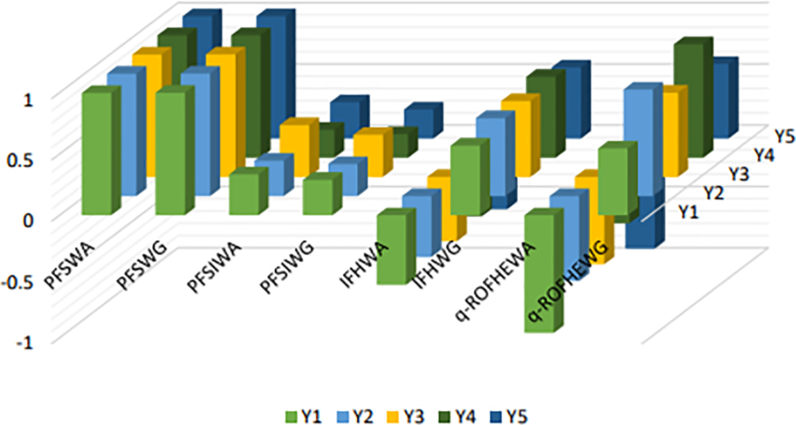
Figure 5: Ranking result of the proposed and existing methods

6  Results and Discussion

According to the study, the aggregation operators suggested in the research use a unique calculation procedure that is distinct from the aggregation operators that have already been used in various scenarios. In the review process, these suggested aggregation operators are considered more acceptable and feasible. In addition, it has been established that the aggregation operators used in previous studies can be used to illustrate the suggested aggregation operators if the lower and upper limits of the degrees of belonging are identical [54,55]. This translates into a more in-depth proposed technique and is capable of collecting more data during the study, which makes it wider and allows a greater range of applications.

7  Conclusion

This paper introduces a novel decision-making technique that utilizes the Einstein agreement operator within the ROFHS environment. Specifically, we investigate two types of operators: Einstein weighted averaging and geometric AOs. We demonstrate that the Einstein weighted averaging operator is highly effective in decision-making scenarios that involve ROFHS numbers under uncertain conditions. Additionally, we explore some of the key implications and relationships of this operator and also discuss some basic properties. Our approach involves utilizing AOs to compute a real tourism carrying capacity based on membership and non-membership data attributes. Our method considers all attribute values and provides a useful and customizable way to assist decision-makers in uncertain situations. Furthermore, our proposed technique is applicable to both ROFHS numbers and ROFS numbers, which accurately reflect uncertainty. To validate our method, we provide a practical example of analyzing tourism carrying capacity. In the future, as we deal with increasingly ambiguous data, we plan to employ the novel aggregation operator to address multi-attribute decision-making challenges.

Acknowledgement: We thank the anonymous reviewers for their insightful comments and suggestions.

Funding Statement: This research was supported by the National Research Foundation of Korea (NRF) grant funded by the Korea government (MSIT) (No. 2021R1A4A1031509).

Author Contributions: The authors confirm contribution to the paper as follows: study conception and design: S. Khan, M. Gulistan; data collection: S. Khan; analysis and interpretation of results: N. Kausar, J. Kim, S. Kadry; draft manuscript preparation: S. Khan, N. Kausar. All authors reviewed the results and approved the final version of the manuscript.

Availability of Data and Materials: No data were used to support this study.

Conflicts of Interest: The authors declare that they have no conflicts of interest to report regarding the present study.

References

1. Li, X., Sun, Y. (2021). Application of RBF neural network optimal segmentation algorithm in credit rating. Neural Computing and Applications, 33(14), 8227–8235. [Google Scholar]

2. Li, X., Sun, Y. (2020). Stock intelligent investment strategy based on support vector machine parameter optimization algorithm. Neural Computing and Applications, 32(6), 1765–1775. [Google Scholar]

3. Li, T., Xia, T., Wang, H., Tu, Z., Tarkoma, S. et al. (2022). Smartphone app usage analysis: Datasets, methods, and applications. IEEE Communications Surveys and Tutorials, 24(2), 937–966. [Google Scholar]

4. Wang, J., Yang, M., Liang, F., Feng, K., Zhang, K. et al. (2022). An algorithm for painting large objects based on a nine-axis UR5 robotic manipulator. Applied Sciences, 12(14), 7219. [Google Scholar]

5. Lu, S., Ding, Y., Liu, M., Yin, Z., Yin, L. et al. (2023). Multiscale feature extraction and fusion of image and text in VQA. International Journal of Computational Intelligence Systems, 16(1), 54. [Google Scholar]

6. Lu, S., Liu, M., Yin, L., Yin, Z., Liu, X. et al. (2023). The multi-modal fusion in visual question answering: A review of attention mechanisms. PeerJ Computer Science, 9, e1400. [Google Scholar] [PubMed]

7. Adak, A. K., Kumar, D. (2020). Spherical distance measurement method for solving MCDM problems under Pythagorean fuzzy environment. Journal of Fuzzy Extension and Applications, 4(1), 29–44. [Google Scholar]

8. Debnath, S. (2021). Fuzzy hypersoft sets and its weightage operator for decision making. Journal of Fuzzy Extension and Applications, 2(2), 163–170. [Google Scholar]

9. Zadeh, L. A. (1965). Fuzzy sets. Information and Control, 8, 338–353. [Google Scholar]

10. Zadeh, L. A. (1973). Outline of a new approach to the analysis of complex systems and decision processes. IEEE Transactions on Systems, Man, and Cybernetics, 3(1), 28–44. [Google Scholar]

11. Klir, G. J., Yuan, B. (1996). Fuzzy sets and fuzzy logic: Theory and applications. Possibility Theory versus Probability. Theory, 32(2), 207–208. [Google Scholar]

12. Yang, S., Nasr, N., Ong, S., Nee, A. (2017). Designing automotive products for remanufacturing from material selection perspective. Journal of Cleaner Production, 153, 570–579. [Google Scholar]

13. Bellman, R. E., Zadeh, L. A. (1970). Decision-making in a fuzzy environment. Management Science, 17(4), 141–273. [Google Scholar]

14. Zimmermann, H. J. (1999). Fuzzy set theory and its applications. USA: Springer Science and Business Media. [Google Scholar]

15. Atanassov, K. T. (1999). Intuitionistic fuzzy sets. In: Studies in fuzziness and soft computing, vol. 35, pp. 1–137. Physica, Heidelberg. [Google Scholar]

16. De, S. K., Biswas, R., Roy, A. R. (2000). Some operations on intuitionistic fuzzy sets. Fuzzy Sets and Systems, 114(3), 477–484. [Google Scholar]

17. Wang, W., Liu, X. (2011). Intuitionistic fuzzy geometric aggregation operators based on Einstein operations. International Journal of Intelligent Systems, 26(11), 1049–1075. [Google Scholar]

18. Rasoulzadeh, M., Edalatpanah, S. A., Fallah, M., Najafi, S. E. (2022). A multi-objective approach based on Markowitz and DEA cross-efficiency models for the intuitionistic fuzzy portfolio selection problem. Decision Making: Applications in Management and Engineering, 5(2), 241–259. [Google Scholar]

19. Tripathi, D. K., Nigam, S. K., Rani, P., Shah, A. R. (2023). New intuitionistic fuzzy parametric divergence measures and score function-based CoCoSo method for decision-making problems. Decision Making: Applications in Management and Engineering, 6(1), 535–563. [Google Scholar]

20. Yager, R. R. (2013). Pythagorean membership grades in multicriteria decision making. IEEE Transactions on Fuzzy Systems, 22(4), 958–965. [Google Scholar]

21. Yager, R. R., Abbasov, A. M. (2013). Pythagorean membership grades, complex numbers, and decision making. International Journal of Intelligent Systems, 28(5), 436–452. [Google Scholar]

22. Adak, A. K., Kumar, D. (2022). Spherical distance measurement method for solving MCDM problems under Pythagorean fuzzy environment. Journal of Fuzzy Extension and Applications, 4(1), 28–39. [Google Scholar]

23. Wei, G., Lu, M. (2018). Pythagorean fuzzy power aggregation operators in multiple attribute decision 511 making. International Journal of Intelligent Systems, 33, 169–186. [Google Scholar]

24. Cuong, B. C., Kreinovich, V. (2014). Picture fuzzy sets. Journal of Computer Science and Cybernetics, 30(4), 409–420. [Google Scholar]

25. Torra, V. (2010). Hesitant fuzzy sets. International Journal of Intelligent Systems, 25(6), 529–539. [Google Scholar]

26. Smarandache, F. (1998). A unifying field in logics. In: Neutrosophy: Neutrosophic probability, set and logic, rehoboth. Santa Fe: American Research Press. [Google Scholar]

27. Smarandache, F. (2018). Physical plithogenic set. In: APS annual gaseous electronics meeting abstracts. Portland, Oregon. [Google Scholar]

28. Yager, R. R. (2016). Generalized orthopair fuzzy sets. IEEE Transactions on Fuzzy Systems, 25(5),1222–1230. [Google Scholar]

29. Molodtsov, D. (1999). Soft set theory—first results. Computers and Mathematics with Applications, 37, 19–31. [Google Scholar]

30. Cagman, N., Enginoglu, S., Citak, F. (2011). Fuzzy soft set theory and its applications. Iranian Journal of Fuzzy Systems, 8(3), 137–147. [Google Scholar]

31. Majumdar, P., Samanta, S. (2011). On similarity measures of fuzzy soft sets. International Journal of Advance Soft Computing and Applications, 3, 1–8. [Google Scholar]

32. Borah, M., Neog, T. J., Sut, D. K. (2012). A study on some operations of fuzzy soft sets. International Journal of Modern Engineering Research, 2(2), 157–168. [Google Scholar]

33. Yang, Y., Tan, X., Meng, C. (2013). The multi-fuzzy soft set and its application in decision making. Applied Mathematical Modelling, 37(7), 4915–4923. [Google Scholar]

34. Smarandache, F. (2018). Extension of soft set to hypersoft set, and then to plithogenic hypersoft set. Neutrosophic Sets and Systems, 22, 168–170. [Google Scholar]

35. Khan, S., Gulistan, M., Wahab, H. A. (2022). Development of the structure of q-Rung orthopair fuzzy hypersoft set with basic operations. Punjab University Journal of Mathematics, 53(12), 881–892. [Google Scholar]

36. Khan, S., Gulistan, M., Kausar, N., Kousar, S., Pamucar, D. et al. (2022). Analysis of cryptocurrency market by using q-Rung orthopair fuzzy hypersoft set algorithm based on aggregation operators. Complexity, 2022, 7257449. [Google Scholar]

37. Khan, S., Gulistan, M., Kausar, N., Pamucar, D., Ozbilge, E. et al. (2023). q-Rung orthopair fuzzy hypersoft ordered aggregation operators and their application towards green supplier. Frontiers in Environmental Science, 10, 2738. [Google Scholar]

38. Khan, S., Gulistan, M., Kausar, N., Pamucar, D., Hong, T. P. et al. (2023). Aggregation operators for decision making based on q-Rung orthopair fuzzy hypersoft sets: An application in real estate project. Computer Modeling in Engineering & Sciences, 136(3), 3141–3156. https://doi.org/10.32604/cmes.2023.026169 [Google Scholar] [CrossRef]

39. Gurmani, S. H., Chen, H., Bai, Y. (2023). Extension of TOPSIS method under q-Rung orthopair fuzzy hypersoft environment based on correlation coefficients and its applications to multi-attribute group decision-making. International Journal of Fuzzy Systems, 25(2), 1–4. [Google Scholar]

40. Qiao, G., Song, H., Prideaux, B., Huang, S. S. (2023). The unseen tourism travel experience of people with visual impairment. Annals of Tourism Research, 99, 103542. [Google Scholar]

41. He, H., Tuo, S., Lei, K., Gao, A. (2023). Assessing quality tourism development in China: An analysis based on the degree of mismatch and its influencing factors. Environment, Development and Sustainability, 60(3), 107. https://doi.org/10.1007/s10668-023-03107-1 [Google Scholar] [CrossRef]

42. Canestrelli, E., Costa, P. (1991). Tourist carrying capacity: A fuzzy approach. Annals of Tourism Research, 18(2), 295–311. [Google Scholar]

43. Xie, X., Tian, Y., Wei, G. (2022). Deduction of sudden rainstorm scenarios: Integrating decision makers’ emotions, dynamic Bayesian network and DS evidence theory. Natural Hazards, 116(3), 2935–2955. https://doi.org/10.1007/s11069-022-05792-z [Google Scholar] [CrossRef]

44. Qi, M., Cui, S., Chang, X., Xu, Y., Meng, Y. et al. (2022). Multi-region nonuniform brightness correction algorithm based on L-channel gamma transform. Security and Communication Networks, 2022(7), 1–9. https://doi.org/10.1155/2022/2675950 [Google Scholar] [CrossRef]

45. Zheng, W., Deng, P., Gui, K., Wu, X. (2023). An abstract syntax tree based static fuzzing mutation for vulnerability evolution analysis. Information and Software Technology, 158, 107194. https://doi.org/10.1016/j.infsof.2023.107194 [Google Scholar] [CrossRef]

46. Yuan, H., Yang, B. (2022). System dynamics approach for evaluating the interconnection performance of cross-border transport infrastructure. Journal of Management in Engineering, 38(3), 1943–5479. [Google Scholar]

47. Fernández-Villarán, A., Espinosa, N., Abad, M., Goytia, A. (2020). Model for measuring carrying capacity in inhabited tourism destinations. Portuguese Economic Journal, 19, 213–241. [Google Scholar]

48. Bertocchi, D., Camatti, N., Giove, S., van der Borg, J. (2020). Venice and overtourism: Simulating sustainable development scenarios through a tourism carrying capacity model. Sustainability, 12(2), 512. [Google Scholar]

49. Maji, P. K., Roy, A. R., Biswas, R. (2002). An application of soft sets in a decision making problem. Computers and Mathematics with Applications, 44(8), 1077–1083. [Google Scholar]

50. Maji, P. K. (2009). More on intuitionistic fuzzy soft sets. In: Rough sets, fuzzy sets, data mining and granular computing, pp. 231–240. Berlin, Heidelberg: Springer. [Google Scholar]

51. Zulqarnain, R. M., Xin, X. L., Siddique, I., Asghar Khan, W., Yousif, M. A. (2021). TOPSIS method based on correlation coefficient under pythagorean fuzzy soft environment and its application towards green supply chain management. Sustainability, 13(4), 1642. [Google Scholar]

52. Zulqarnain, R. M., Xin, X. L., Garg, H., Ali, R. (2021). Interaction aggregation operators to solve multi criteria decision making problem under pythagorean fuzzy soft environment. Journal of Intelligent and Fuzzy Systems, 41(1), 1151–1171. [Google Scholar]

53. Zulqarnain, R. M., Siddique, I., Ali, R., Pamucar, D., Marinkovic, D. et al. (2021). Robust aggregation operators for intuitionistic fuzzy hypersoft set with their application to solve MCDM problem. Entropy, 23(6), 688. [Google Scholar] [PubMed]

54. Hussain, A., Ali, M. I., Mahmood, T., Munir, M. (2020). q-Rung orthopair fuzzy soft average aggregation operators and their application in multicriteria decisionmaking. International Journal of Intelligent Systems, 35(4), 571–599. [Google Scholar]

55. Hayat, K., Shamim, R. A., AlSalman, H., Gumaei, A., Yang, X. P. et al. (2021). Group generalized q-Rung orthopair fuzzy soft sets: New aggregation operators and their applications. Mathematical Problems in Engineering, 2021, 1–6. [Google Scholar]