Prediction of Porous Media Fluid Flow with Spatial Heterogeneity Using Criss-Cross Physics-Informed Convolutional Neural Networks

1  Introduction

Flow and transport in porous media play a crucial role in a variety of subsurface energy and environmental applications, such as reservoir recovery, carbon sequestration, etc. Many of these problems can be characterized as partial differential equations derived from the principles of conservation. However, due to the intricate nature of PDEs and the absence of rigorous theoretical analysis techniques, the approximation of most PDEs is only resorted to based on discretized methods, such as finite difference, finite volume, and finite element. After decades of development, these methods have become robust and flexible. However, for considerably large problems, numerical simulations can become increasingly slow and sometimes prohibitively so [1]. Moreover, multiple simulation runs are required to inverse problems, conduct sensitivity analyses, and optimize a project’s design. Recently, surrogate models to traditional numerical models have been widely employed in the field of reservoir development, including reduced-order methods [2–6], deep learning methods [7–15], and Gaussian process [16,17], which provide a rapid numerical model approximator to efficiently solve inverse problems, optimization problems.

In recent years, with the increase in GPU computing power and the generalization of deep learning frameworks [18], the application of deep learning in petroleum engineering has garnered significant interest due to its powerful nonlinear approximation and data assimilation capabilities [19–25]. Despite the relentless development of the data-driven method, there are still some problems in dealing with scientific and engineering problems. The traditional data-driven method usually requires a great deal of quality data, more importantly, ignores the physical principles underlying the research problem, which results in predictions that may be physically inconsistent or implausible [26]. To enhance the model's predictive consistency with first principles, a unified model is needed to naturally leverage theoretical constraints and any useful prior knowledge [27]. Raissi et al. [28] proposed the physics-informed neural networks (PINNs) which can seamlessly integrate observational data and physics laws by incorporating the PDEs, boundary conditions, initial conditions, and observational data into the loss function to construct a hybrid physics-constrained loss function based on an automatic differentiation algorithm [26,29–31]. Based on the PINN framework, many researchers have proposed many interesting variants for specific problems [32–36]. Yan et al. [27] developed a gradient-based deep neural network (GDNN) for modeling multiphase flow in porous media at geologic CO2 storage sites, which eliminates nonlinearity by decomposing nonlinear PDEs into elementary differential operators. Li et al. [37] proposed a Theory-Guided Neural Network (TGNN) to predict the state variables of two-phase by incorporating besides the governing equations but also the expert knowledge and engineering controls into the loss function. Jagtap et al. [38] proposed a conservative physics-informed neural network (cPINN) for solving nonlinear PDEs by decomposing the computational domain into different sub-domains and enforcing the flux continuity in the strong form along the sub-domain interfaces. Park et al. [39] constructed a hybrid model for optimum unconventional field development by combining unconventional reservoir uncalibrated priors and data generated by a numerical simulator. To solve the two-phase immersible flow problem governed by the Buckley-Leverett equation [40,41], they used physics-informed neural networks and obtained a physical solution by adding a diffusion term or an observational amount to the PDEs.

The auto-differentiation-based PINN model is suitable for a homogeneous scientific problem, however, it is unclear how AD can enforce flux continuity across boundaries between cells of different properties where spatial heterogeneity is represented by grid cells with different physical properties [42]. In this work, we try to combine the physics laws with data to simulate the single and two-phase flow in porous media using convolutional neural networks. The finite difference method (FDM) is used to approximate the governing equation residual, which allows flux continuity between cells to be rigorously defined. A predefined 2D convolution layer with a criss-cross convolution kernel is introduced to enable and enforce flux continuity and express the discretized governing equations, harmonic mean of permeability, and upstream-weighted differencing schemes. Moreover, the proposed method has also been compared against the state-of-the-art PINN. The numerical reference results evince the effectiveness of the proposed method over the PINN.

The remainder of this paper is structured as follows. Section 2 introduces the conservation equation of multiphase darcy flows in porous media in petroleum reservoirs and criss-cross physics-informed convolutional neural networks. Section 3 validates the model on single and two-phase flow in the heterogeneous reservoir. Finally, discussions and conclusions are given in Section 4.

2  Methodology

2.1 Single and Multiphase Darcy Flows in Petroleum Reservoirs

In this study, we introduce the general oil-water two-phase Darcy flow model (Single phase model can be obtained by simplifying the two-phase model) in the porous media. We consider the fluids are slightly compressible and immiscible, and there is no mass transfer between the phases. The governing equation can be written as follows:

∇(ρwkkrwμw∇pw)+qw=∂(ϕρwSw)∂t∇(ρokkroμo∇po)+qo=∂(ϕρoSo)∂t(1)

where the ρw and ρo are the density of water and oil; k, krw Eq. (2) and kro Eq. (3) are the absolute permeability, the relative permeability of oil and water, respectively; μw and μo are the water and oil viscosity; po and pw are the pressure of oil phase and water phase; Sw and So are the saturation of water and oil; qw and qo are the source/sink term of water and oil phase; ϕ is the porosity of porous media. And in this work, there is no capillary pressure so pw=po.

krw=(Sw−Swi1−Swi−Sor)2(2)

kro=(1−Sor−Sw1−Swi−Sor)2(3)

where the Swi and Sor irreducible water saturation and residual oil saturation, respectively. Since no mass transfer occurs between the phases, we can use volume factor and compressibility to rewrite the governing equations as follows:

∇(krwkBwμw∇pw)+qw=ϕSwBwref(Cϕ+Cw)∂pw∂t+ϕBwref∂Sw∂t∇(krokBoμo∇po)+qo=ϕSoBoref(Cϕ+Co)∂po∂t+ϕBoref∂So∂t(4)

where the Bw and Bo are the volume factor of water and oil, respectively; Cϕ, Cw and Co are the compressibility of the rock, water, and oil, where the Bref is the volume factor at the reference pressure. When simplified to one phase, the equation can be written as follows:

∇(kμB∇p)−q=ϕCtBref∂p∂t(5)

2.2 Convolutional Neural Network (CNN)

The convolutional neural network (CNN or ConvNet) is a deep learning structure that can learn directly from image data without manually extracting features [43]. CNNs are particularly well suited for finding patterns in images to recognize objects, faces, and scenes. Such networks also work well for classifying some non-image data, such as audio, time series, and signal data. Despite there are many kinds of new and complex variants, CNNs still rely on convolution layers, which are composed of convolutional kernels or filters with learnable biases and weights. It reduces the number of parameters required by the convolutional layer by sharing the same convolutional kernel across all spatial locations. For illustration, suppose that the input tensor is:

X∈RM×N(6)

where M and N denote the dimensions of the input, and xi,j is the value of input tensor X at the position (i,j). Consider a specific convolutional kernel:

ω∈Rkh×kw(7)

where kh and kw are the dimensions of the convolutional kernel, ωc,d denotes the weight value at the position (c,d). The feature map can be expressed as follows:

ui,j=∑c=1kh∑d=1kwxi⋅s1−1+c,j⋅s2−1+d⋅ωc,d+b(8)

where s is stride which is a parameter of the neural network’s filter that modifies the amount of movement over the image, b is the bias of the convolutional kernel.

2.3 Criss-Cross Physics-InFormed Convolutional Neural Networks

Despite the tremendous advancements the traditional data-driven method has made, it is inevitably considered to be a ‘black box’, which means that the system does not embody any physical meaning of the dataset and the predictions may be physically inconsistent or implausible [26]. In this work, a criss-cross physics-informed convolutional neural network is proposed for modeling flow in porous media, which can be trained with limited training data, and scientific theories can be incorporated seamlessly. Consider a specific petroleum reservoir problem, the governing equation Eq. (1) can be discretized with the finite difference method:

left=Tαx,i+1/2n+1pαi+1n+1+Tαx,i−1/2n+1pαi−1n+1+Tαx,j+1/2n+1pαj+1n+1+Tαx,j−1/2n+1pαj−1n+1+(Tαx,i+1/2n+1+Tαx,i−1/2n+1+Tαx,j+1/2n+1+Tαx,j−1/2n+1+ϕSαVi,j(Cϕ+Cα)BαrefΔt)pαi,jn+1+qα=bpαi+1n+1+apαi−1n+1+dpαj+1n+1+cpαj−1n+1+epαi,jn+1right=Vi,jϕBαrefSαi,jn+1−Sαi,jnΔt−ϕSαVi,j(Cϕ+Cα)BαrefΔtpαi,jn(9)

where α is o for oil and w for water; Ti±1/2n+1 and Tj±1/2n+1 denote the transmissibility between adjacent cells; the subscript i, j and n denote the indexes of discretized grids in the horizontal, vertical, and temporal dimension, respectively; the permeability is taken as harmony mean (Eq. (10)); the volume factor and mobility are taken as upstream weight (Eq. (11)); the well can be modeling by Peacemen equation (Eq. (12)) [44].

ki±1/2,j=2×ki±1,j×ki,jki±1/2,j+ki,j(10)

(kkrαBαμα)i±1/2=λi±1/2={λi±1λi      if pi±1 ≥ pi     if pi±1 < pi(11)

q=2πkhμ(ln⁡(re/rw)+S)(pw−pij)(12)

where k is permeability, h is the thickness of the reservoir, μ is the fluid viscosity, pij is the well-containing grid pressure, pw is the bottom hole flow pressure, the equivalent radius equals re=0.20788Δx, rw is the radius of the wellbore, and S is skin effects.

To achieve the seamless enforcement of flux continuity and integration of physical meaning into CNN, a predefined 2D convolutional layer with a criss-cross kernel layer is proposed, specifically as shown in Fig. 1.

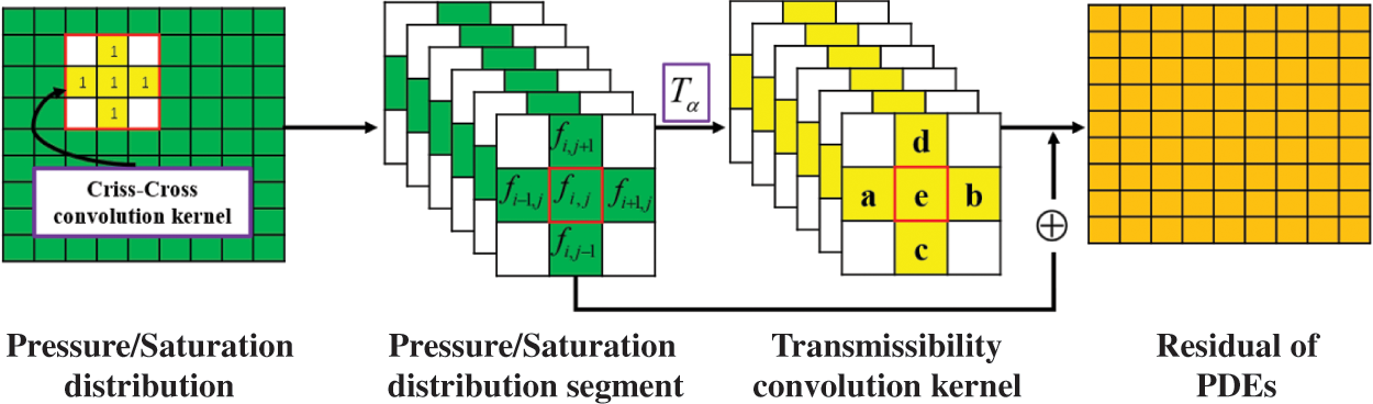
Figure 1: Predefined 2D convolutional layer

Therefore the discretized residual of the control equation (Eq. (9)) can be expressed as follows:

MSEpde=1Nu∑i=1Nu[criss−cross−kernel⋅p^αn+1⋅Transmissibility−kernel(p^αn+1)+qi,j−VijϕBαrefS^αn+1−S^αnΔt+ϕS^αnVi,j(Cϕ+Cα)BαrefΔtp^αn]2(13)

where MSEpde is the loss associated with the residual of governing equations; Nu is the total number of collocation points of the governing equation; p^αn+1 is the pressure matrix of output at time n + 1 for phase α; S^αn+1 is the saturation matrix of output at time n+1 for phase α.

For boundary condition constraints, the Cov2D operation of CNN is used to implement the constant pressure and closed boundary conditions, as shown in Fig. 2.

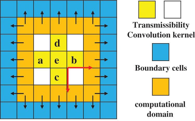
Figure 2: The implementation of boundary conditions

The initial conditions are added to the loss function as a penalty item (Eq. (14)).

MSEic=1Nic∑i=1Nic(S^wic−Swic)2+1Nic∑i=1Nic(p^wic−pwic)2(14)

where MSEic is the loss associated with the residual of initial conditions; Nic is the total number of collocation points of initial condition; S^wic and Swic are the saturation matrix of output and reference value, respectively; p^wic and pwic are the pressure matrix of output and reference value.

Similar to conventional neural networks, the MSE between prediction and truth data can also be added to the loss function of neural networks.

MSEdata=1Ndata∑i=1Ndata(S^wn−Swn)2+1Ndata∑i=1Ndata(p^wn−pwn)2(15)

where MSEdata is the loss associated with the residual of data match; Ndata is the total number of label data; S^wn and Swn are the water saturation matrix of output and label data, respectively; p^wn and Pwn are the water pressure matrix of output and label data.

As a result, the total loss function can be as follows:

MSE=MSEpde+MSEic+MSEdata(16)

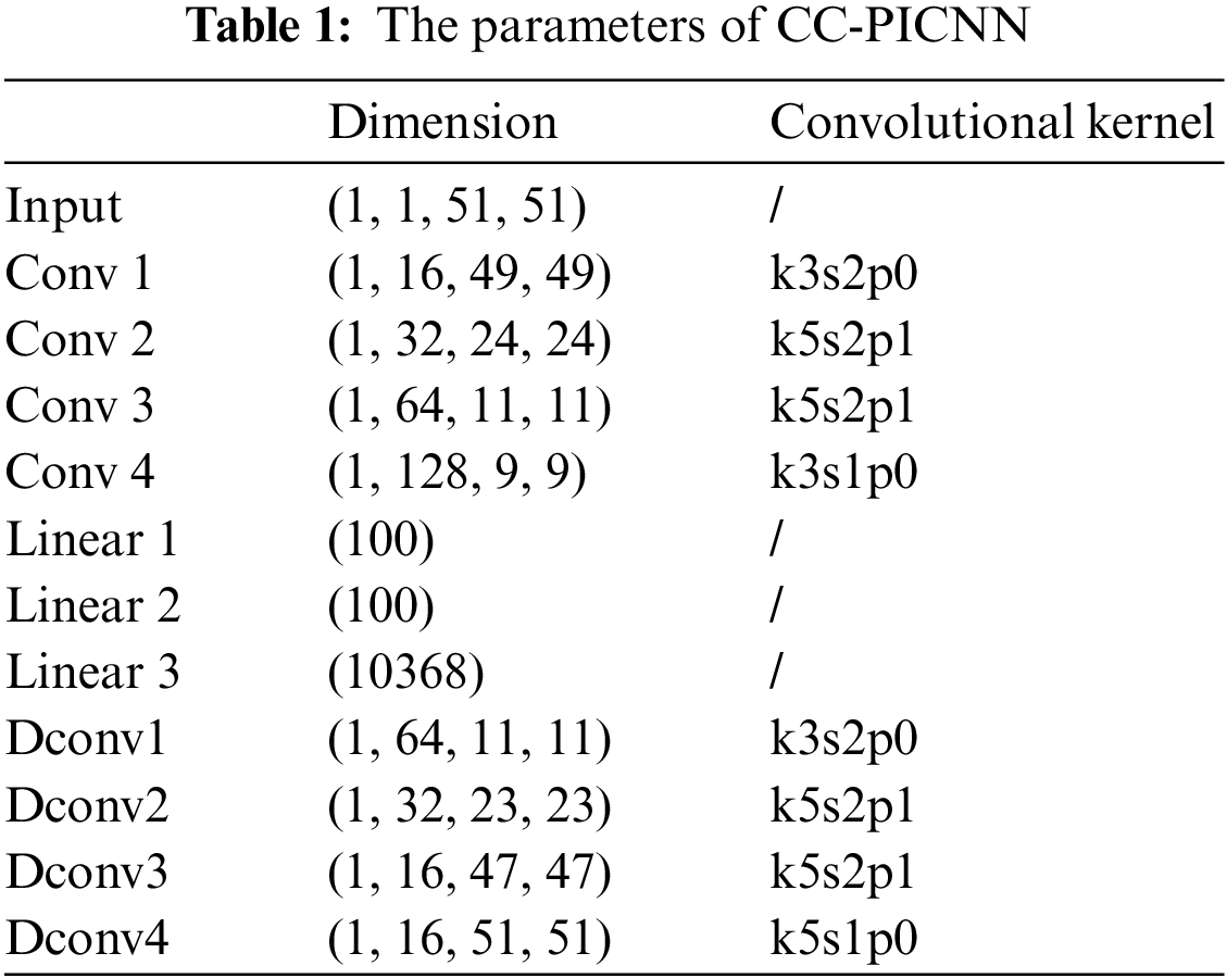
Typically, weights are assigned to each subterm of the loss function. However, there is no systematic analysis of weight determination or optimization in the literature, and these weights are commonly tuned by hand based on experience or trial and error. They remain constant during the training process [45]. In this work, we use a trick to alleviate the troublesome process of tuning the weights to a certain extent. We adjust the timing of putting different loss items into network training. Specifically, instead of training all objects at the same time, we first train the initial conditions and data matching in the first stage, and subsequently add the rest of the items. This can be done because the learning of the laws of physics and other parts is based on initial conditions. Subsequently, the criss-cross physics-informed convolutional neural networks can be instantiated via minimization of the total loss function. Such an approach inherently capitalizes on the discretized control equation, initial conditions, and boundary conditions to guarantee its accuracy and physical consistency of output. The structure and parameters of the criss-cross physics-informed neural network model are illustrated in Fig. 3 and Table 1. In the context of two-phase flow, the interdependence of pressure and saturation necessitates a coupled solution. Accordingly, to alleviate the burden of training, two distinct networks are employed to address pressure and saturation, respectively. Through imposing physical constraints, the aforementioned networks are subsequently linked. In contrast, when tackling the single-phase scenario, solely the pressure network is trained, with the saturation network being discarded.

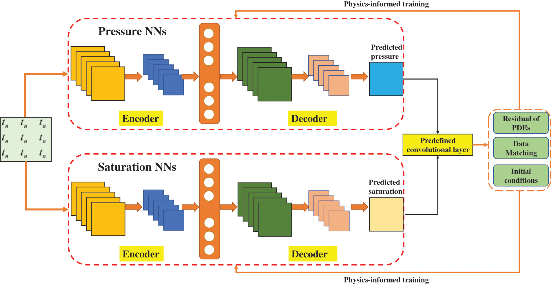
Figure 3: The structure of the criss-cross physics-informed convolutional neural networks

3  Test Cases

In this section, we evaluate the performance of the criss-cross physics-informed convolutional neural network by assessing it on two heterogeneous reservoir problems: a single-phase problem and an oil-water two-phase problem.

3.1 Single-Phase Heterogeneous Reservoir Problem

Initially, we examine a 2D heterogeneous reservoir problem, which is derived from an actual block, and labeled data is generated through numerical simulations. The geological model features closed boundaries on all sides. The initial pressure is 300 bar. The dimension of the reservoir model is 510m×510m×10m and the domain is discretized into 51×51 grid blocks with Δx=Δy=10m. The permeability field is depicted in Fig. 4. The porosity is 0.2 everywhere. The water and rock are incompressible, and the oil compressibility and the volume factor at the reference pressure are 0.0045 bar−1 and 1.12. The water and oil viscosity are 0.3 and 3. The reservoir is simulated for 50 months with ΔT=1month. The three production wells producing at a constant rate of 50, 30 and 20 m3/d respectively located in (510, 510), (210, 210), (770, 310).

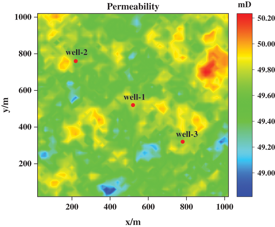
Figure 4: Permeability field

The CC-PINN takes a single-channel input, represented by the time matrix, and produces a single-channel output in the form of the pressure field image. The network architecture is illustrated in Fig. 3 and comprises an encoder and a decoder, each containing four convolutional layers. The Sigmoid Linear Unit (SiLU) activation function and the Adam optimizer, with a learning rate decay strategy, are employed for model training, using an initial learning rate of 0.001 a decay rate of 0.1, and an epoch of 5000. The predictive performance of the CC-PINN model is evaluated using two metrics: the coefficient of determination and the relative L2 error, as described by Eqs. (17) and (18), respectively.

R2=1−∑i=1N(u^i−ui)2∑i=1N(ui−ui¯)2(17)

L2=‖uθ−u‖2‖u‖2(18)

where the u^i and ui are the prediction and truth value; u¯i is the average value of the truth value; N is the number of evaluation points; ‖⋅‖2 denotes the standard Euclidean norm.

In this study, the data of the initial 65-time steps were extracted as the training dataset to develop a predictive model for the pressure response over the subsequent 35-time steps response. Subsequently, we established the geological and mathematical models, along with the requisite network configurations, to train and evaluate the CC-PINN model. The predicted pressure of CC-PINN at time step 75 and 100 are illustrated in Figs. 5b and 6b, it can be seen that predicted pressure by CC-PICNN is very close to the reference solutions with mean absolute differences below 0.1, and negligible difference visually. Moreover, the predictions of pressure from the PINN at time step 75 and 100 are shown in Figs. 5c and 6c. It demonstrates that the single-phase flow in porous media with spatial heterogeneity problems can be handled well by CC-PINN.

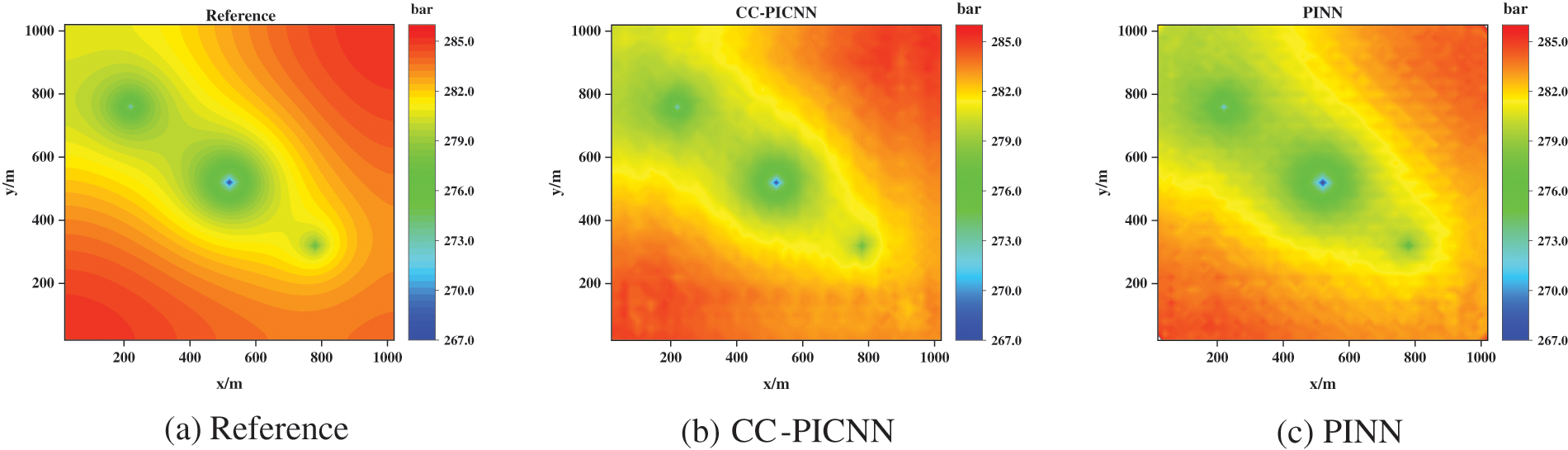
Figure 5: Pressure fields obtained by numerical simulation (left), CC-PICNN (middle), and PINN (right) at T = 75

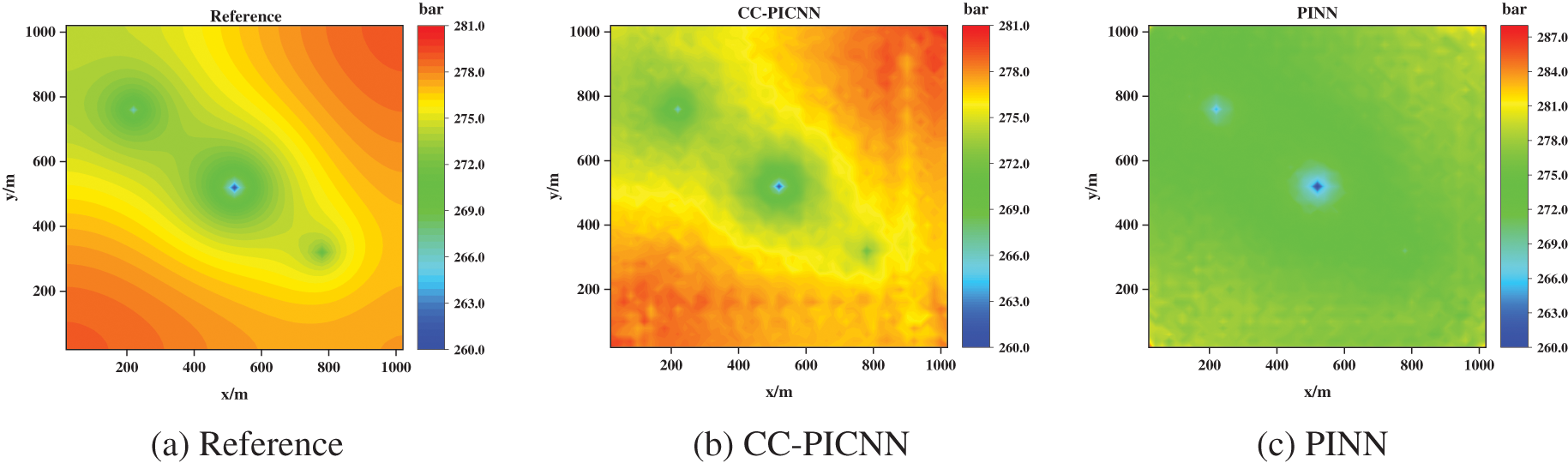
Figure 6: Pressure fields obtained by numerical simulation (left), CC-PICNN (middle), and PINN (right) at T = 100

The histogram of relative L2 error (a) obtained by CC-PICNN and PINN on the test dataset is shown in Fig. 7, although the relative L2 error and R2 score metric reach the same level, the CC-PICNN is more precise and smoother, since the spatial heterogeneity of permeability is better satisfied and expressed by a predefined convolutional layer. However, for PINN, the error tends to increase as time evolves, probably due to the cumulative effect of the error.

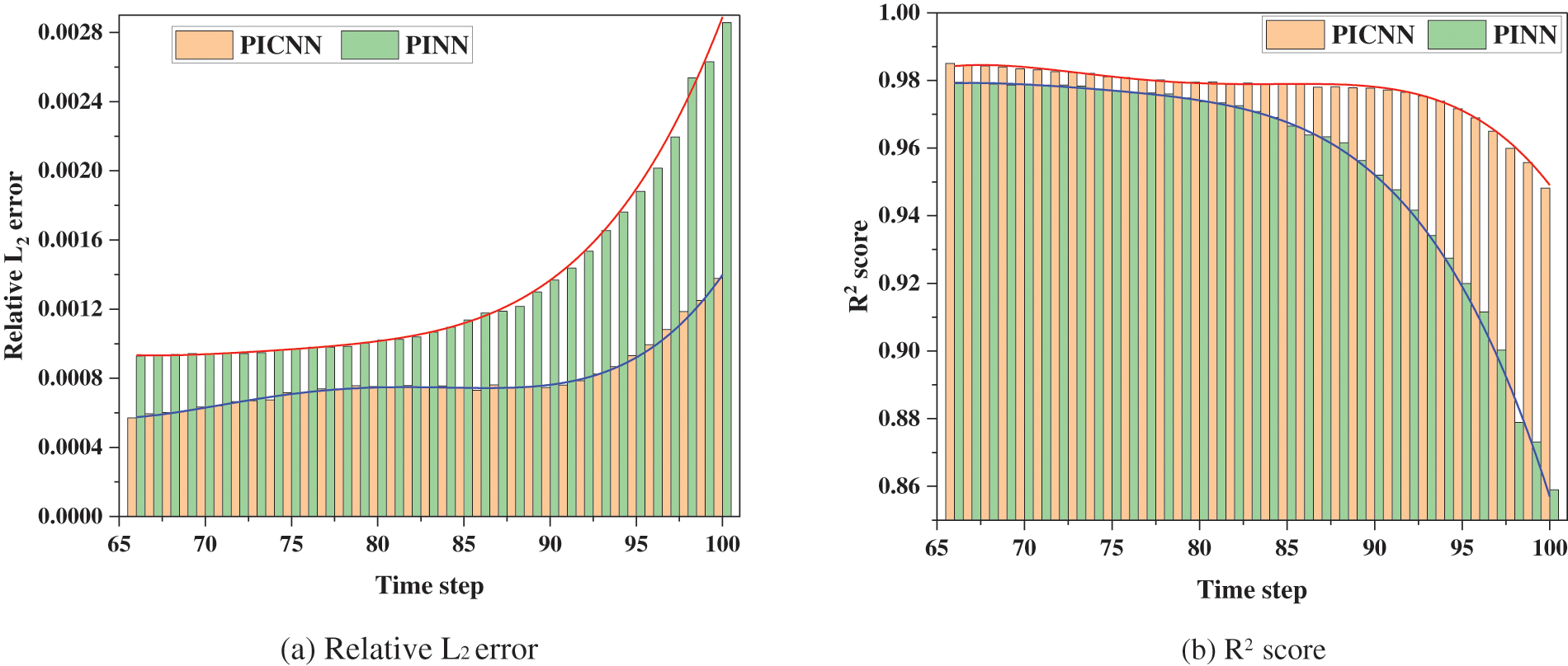
Figure 7: The relative L2 error (a) and R2 score (b) obtained by CC-PICNN and PINN on the test dataset

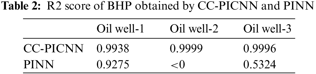
The results show the satisfactory accuracy of the CC-PINN and superior performance compared with the PINN model. The accuracy of CC-PINN is further validated by comparing the bottom-hole pressure (BHP) curves to reference numerical solutions and PINN. As shown in Fig. 8, the curve of bottom-hole pressure obtained from the CC-PINN model almost overlaps with the reference numerical solutions compared to the PINN. The non-convergence of the predicted curve, as determined by the PINN, can be attributed to the inadequacy of convergence in the well-containing grid pressure. This results in a discrepancy between the predicted curve and the reference curve. Notably, all three models employ the same well index. And the comparison of the predictive accuracy of CC-PICNN and PINN is shown in Table 2. The comparison work demonstrated that CC-PICNN can better handle the strong nonlinear conditions of a source-sink term with well control conditions of the constant liquid rate at the same number of iterations.

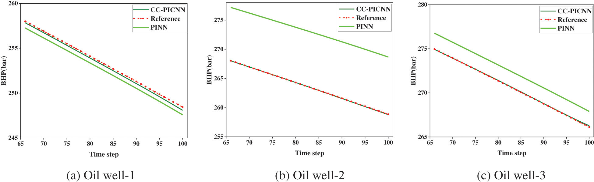
Figure 8: The BHP obtained by numerical simulation, CC-PICNN, and PINN

3.2 Oil-Water Two-Phase Heterogeneous Reservoir Problem

In this sub-section, the CC-PINN model is demonstrated in the context of a two-phase heterogeneous reservoir scenario. Unlike the single-phase problem, the governing equations (Eq. (5)) for two-phase flow represent a coupled system of pressure and saturation, thereby inducing interferences during backpropagation if a singular neural network is employed for training. Therefore, two distinct networks are adopted to tackle pressure and saturation separately, as depicted in Fig. 3. By enforcing physical constraints, the two networks are interdependent. Both networks adhere to a standard configuration comprising four convolutional layers, with an encoder and decoder component.

The geological model to be solved is a domain covering 510 × 510 × 10 m3 with four no-flow boundary conditions. The coordinates of the injection and production wells are (5, 5) and (505, 505), respectively. In this work, we assume that the rock and fluid are incompressible. The porosity is 0.2 and the permeability is shown in Fig. 9. The reservoir’s initial conditions comprise a pressure of 250 bar, with initial water saturation and irreducible water saturation of 0.2. The reservoir is simulated for 100 months with ΔT=1month. The injection and production wells exhibit a constant liquid volume of 50 m3/day and a constant well bottom pressure of 150 bar, respectively. The parameter configuration utilized in CC-PINN remains consistent with the single-phase problem in Section 3.1.

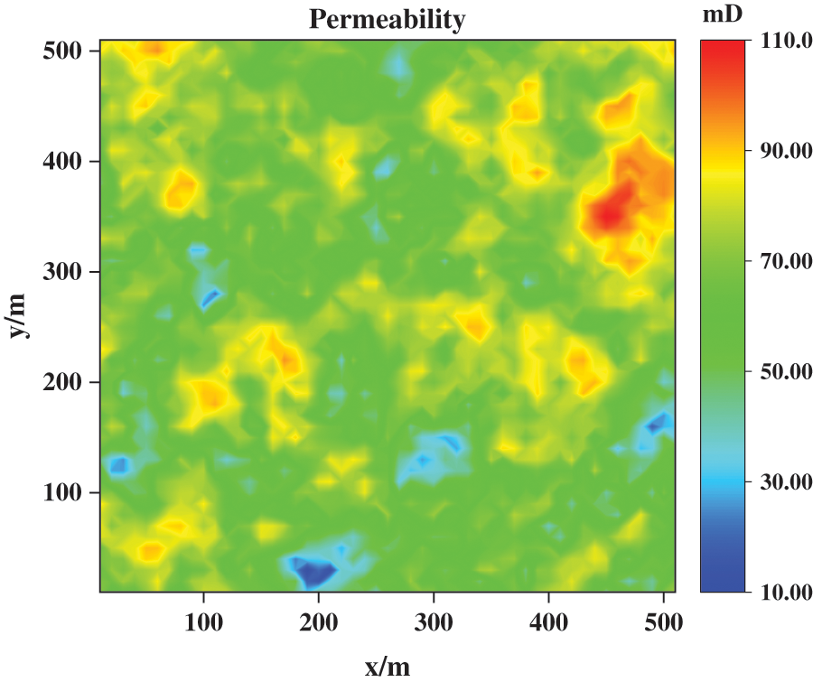
Figure 9: Permeability field

The predicted pressure and water saturation of CC-PINN at time step 75 and 100 are illustrated in Figs. 10b, 10e, and 11b, 11e, it can be seen that the pressure and saturation distribution obtained by the CC-PINN is in good agreement with the reference numerical solution, however, the error increases near the well and saturation font where the pressure gradient or water saturation changes dramatically. Moreover, the predictions of pressure and water saturation from the PINN model at time step 75 and 100 are shown in Figs. 10c, 10f, and 11c, 11f. Based on experimental results, it is evident that the pressure distribution exhibited by the CC-PICNN model conforms more closely to the laws of physics.

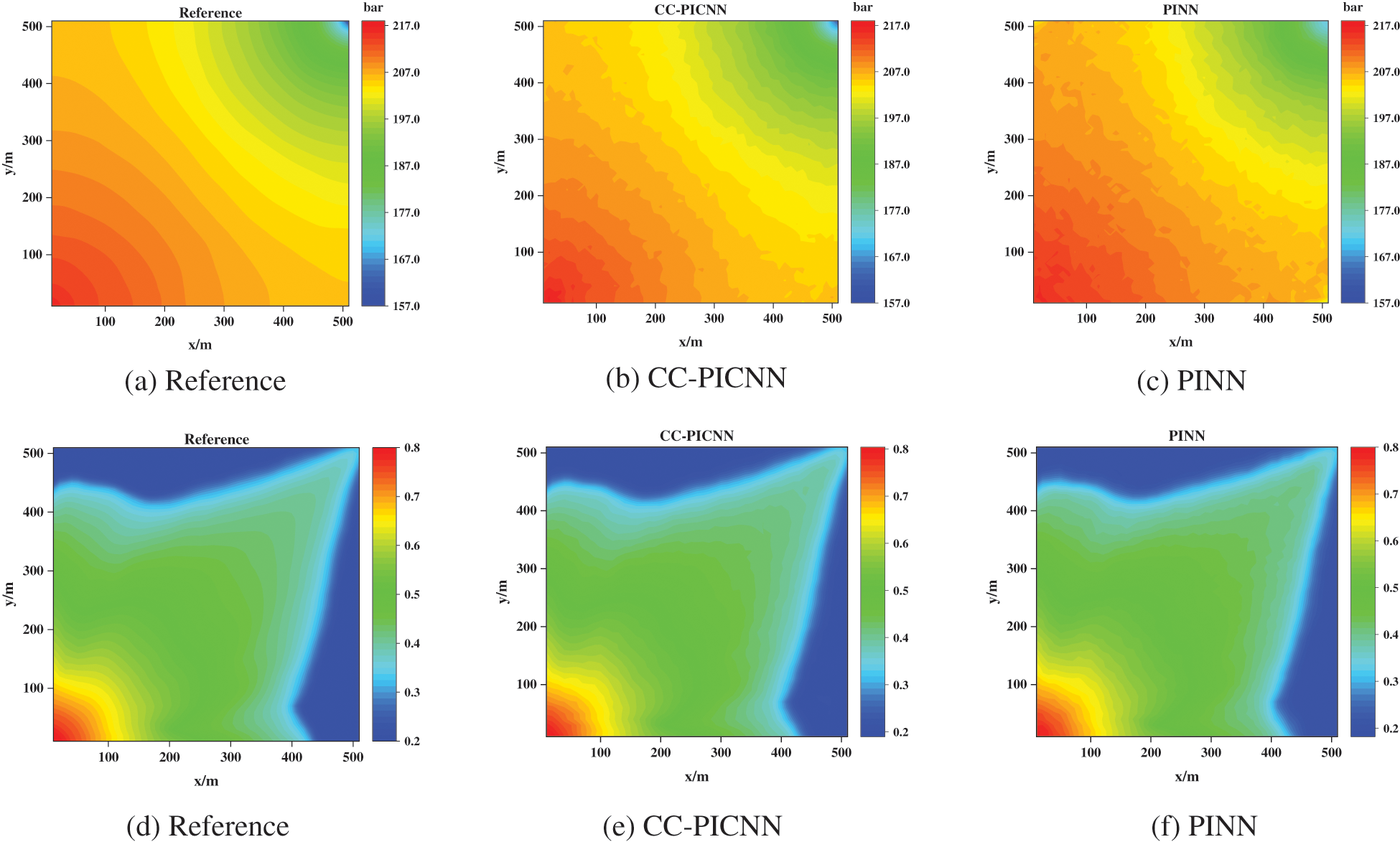
Figure 10: Pressure (the first row) and water saturation (the second row) fields of numerical simulation benchmark (left column), CC-PICNN (middle column), and PINN (right column) at T = 75

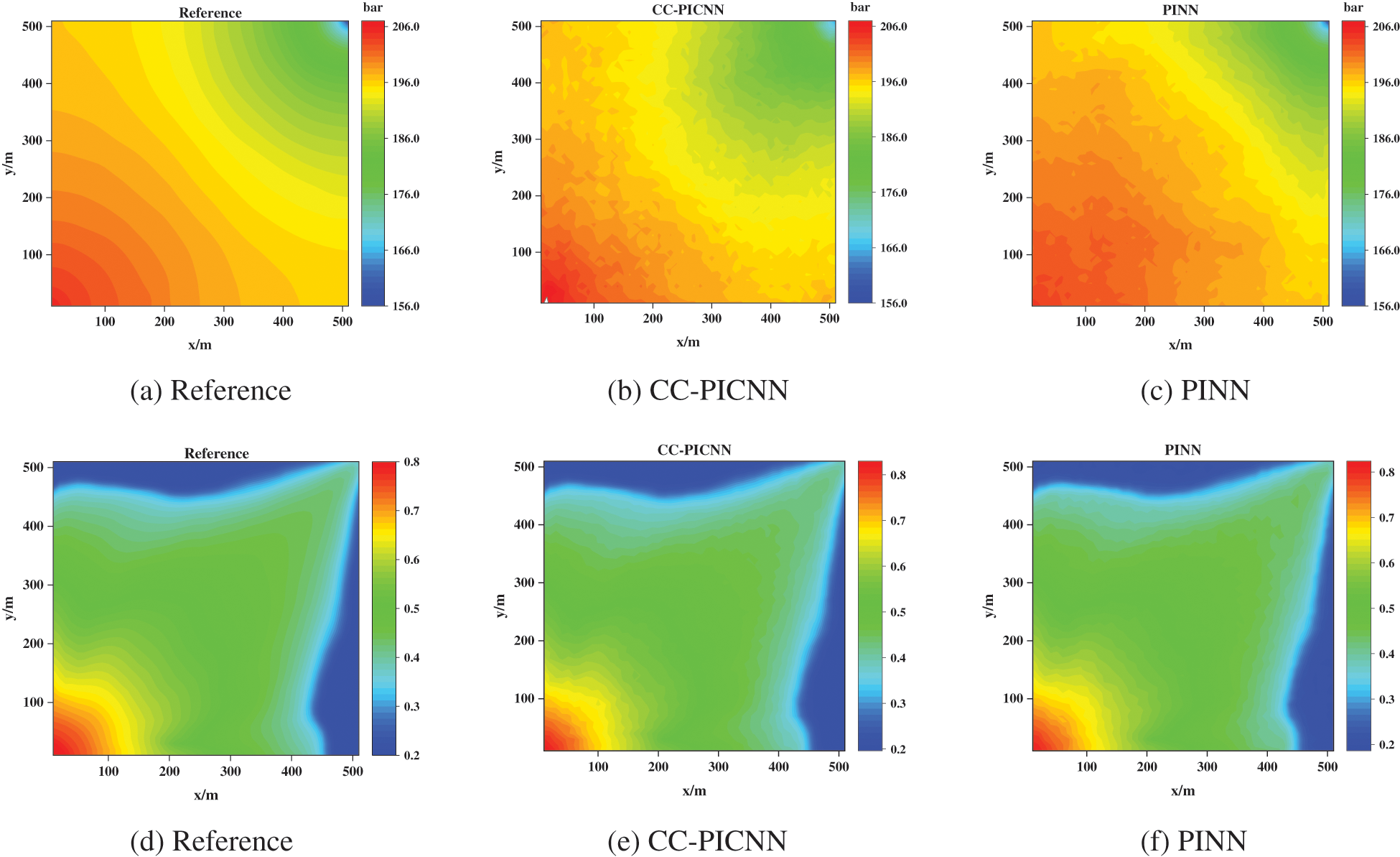
Figure 11: Pressure (the first row) and water saturation (the second row) fields of numerical simulation benchmark (left column), CC-PICNN (middle column), and PINN (right column) at T = 100

Based on the predicted data, it is observed that the PINN model exhibits an evolution over time, as evidenced by the histograms of R2 scores and relative L2 errors for the 35 predicted test time steps by CC-PINN and PINN in Fig. 12. Specifically, a higher accuracy curve indicates that the CC-PICNN is better at correctly regressing instances, both PINN and CC-PICNN model display an exponential increase in L2 errors and a corresponding decrease in R2 scores, which could potentially be attributed to error accumulation. The aforementioned findings are consistent with the established literature on error propagation in machine learning models.

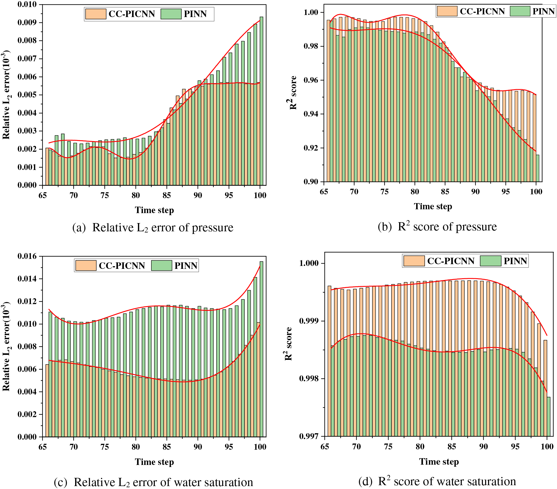
Figure 12: The histograms of R2 scores and relative L2 errors for the 35 predicted test time steps by CC-PINN and PINN

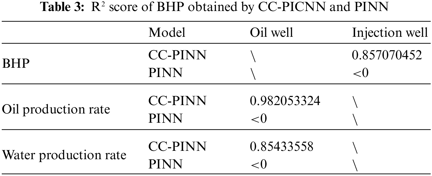
The accuracy of CC-PINN is further validated by comparing the bottom-hole pressure (BHP) of the injection well and liquid production rate of oil well curves to the PINN model and reference numerical solutions benchmark, as shown in Fig. 13. And the comparison of the predictive accuracy of CC-PICNN and PINN is shown in Table 3. A lower loss of the curve obtained by CC-PICNN indicates that the model is better at minimizing the rate error.

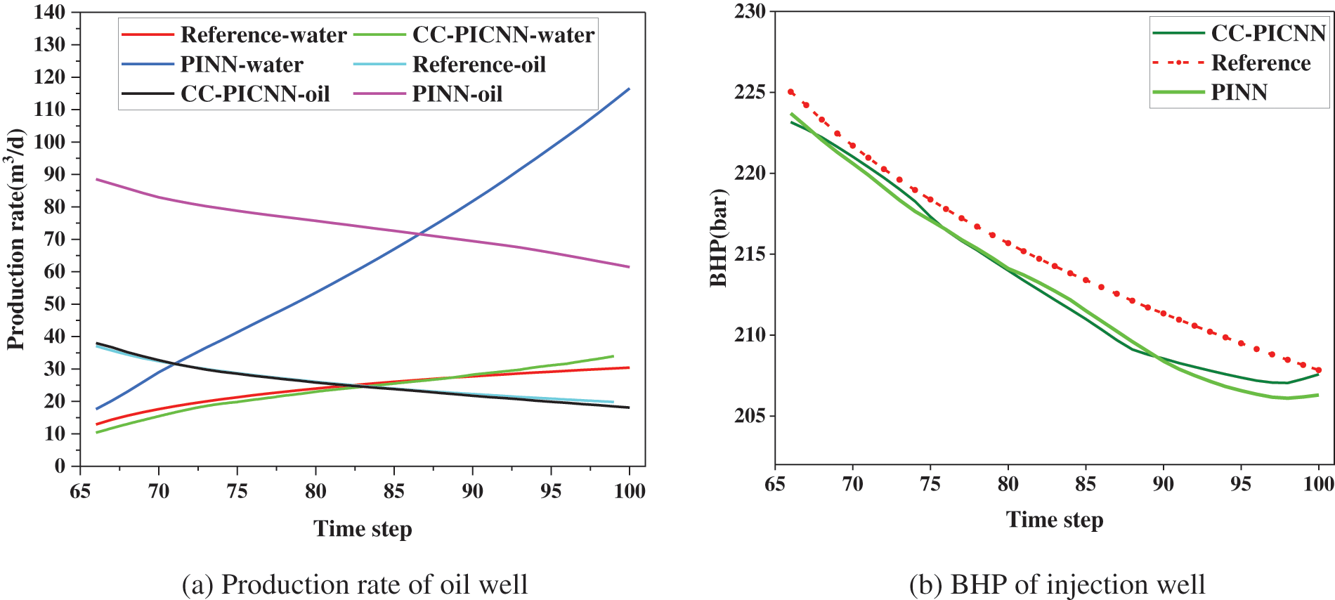
Figure 13: Production rate of oil well (left) and BHP of injection well (right) obtained by numerical simulation, CC-PICNN, and PINN

The oil production rate and water production rate curves obtained by CC-PICNN exhibit a remarkable degree of congruence with the reference numerical solutions, as opposed to those obtained by PINN. Specifically, the non-convergence of the predicted curve obtained by PINN can be attributed to the inadequacy of convergence in the well-containing grid pressure and water saturation. The non-convergence can be ascribed to the inadequate prediction of well grid pressure and non-adherence of two-phase saturation to the conservation condition of summing up to unity. This leads to inaccuracies in production pressure difference and relative permeability, ultimately culminating in substantial errors in the resultant production curve.

Although showing good ability in addressing spatially heterogeneous problems, the current framework has several limitations, and many technical challenges are still present. Firstly, the data used in this paper are derived from numerical simulations, which may not always be applicable to scientific problems. Furthermore, the acquisition of numerical simulation data is resource-intensive, which may limit the practical application of the model. Therefore, it is crucial to explore methods that use little or no labeled data in future research. Secondly, the CNN-based physics-informed model in this paper can only handle regular boundaries at present and cannot solve complex boundary conditions. This is a technical challenge that necessitates further research and development.

4  Conclusion

In this work, a criss-cross physics-informed convolutional neural network (CC-PINN) is proposed for predicting porous media fluid flow with spatial heterogeneity. A 2D convolutional layer with a criss-cross convolutional kernel is introduced to achieve the seamless enforcement of flux continuity and integration of physical meaning into CNN. The layer is designed to enable the direct use of powerful classic CNN backbones for expressing transmissibility between adjacent cells, discretized residuals of PDEs, harmonic means of permeability, upstream-weighted differencing schemes, and boundary conditions. The introduction of this layer is motivated by the need to ensure accurate representation and conservation of information in the discretized domain. The criss-cross convolutional kernel utilized in this layer facilitates the computation of the relevant physical quantities and guarantees the preservation of their inherent properties in the CNN model. The initial conditions, and discretized PDEs residual expressed by the criss-cross convolutional kernel are imposed in the loss function as physical penalty terms for data match loss, additionally, the boundary conditions are seamlessly integrated into the training process by padding operation in CNN. In essence, the solving process of PDEs in numerical simulators is replaced by the training procedure of deep learning, and the solving scheme can be learned by the network. Once trained, the CC-PINN can be used to predict future pressure and saturation distributions. The effectiveness and merit of the proposed CC-PINN have been demonstrated by solving several dynamic subsurface flow instances in reservoir porous media, encompassing a spectrum of heterogeneous problems, ranging from single-phase to two-phase complexities. Through numerical analysis as a benchmark, we compared the proposed CC-PICNN model with the state-of-the-art PINN model. The findings demonstrate that the CC-PINN exhibits a faster convergence rate than the PINN model, and the accuracy of the CC-PINN model surpasses that of the PINN model, provided that the total training dataset and iteration number remain constant. These results highlight the superiority of the proposed CC-PINN model over the existing state-of-the-art PINN model for the prediction of porous media fluid flow with spatial heterogeneity.

Acknowledgement: None.

Funding Statement: This work was supported by the National Natural Science Foundation of China (No. 52274048), Beijing Natural Science Foundation (No. 3222037), the CNPC 14th Five-Year Perspective Fundamental Research Project (No. 2021DJ2104), and the Science Foundation of China University of Petroleum, Beijing (No. 2462021YXZZ010).

Author Contributions: The authors confirm contribution to the paper as follows: study conception and design: Liang Xue, Jiangxia Han; data collection: Ying Jia, Mpoki Sam Mwasamwasa, Felix Nangukar; analysis and interpretation of results: Charles Sangweni, Hailong Liu, Qian Li; draft manuscript preparation: Jiangxia Han, Liang Xue. All authors reviewed the results and approved the final version of the manuscript.

Availability of Data and Materials: The raw data supporting the findings of this study are available from the https://drive.google.com/drive/folders/1pbX34hKxOxp9wajg5qS8VAtoUCghwi57?usp=sharing.

Conflicts of Interest: The authors declare that they have no conflicts of interest to report regarding the present study.

References

1. Ertekin, T., Sun, Q. (2019). Artificial intelligence applications in reservoir engineering: A status check. Energies, 12(15), 2897. https://doi.org/10.3390/en12152897 [Google Scholar] [CrossRef]

2. Xiao, D., Lin, Z., Fang, F., Pain, C. C., Navon, I. M. et al. (2017). Non-intrusive reduced-order modeling for multiphase porous media flows using Smolyak sparse grids. International Journal for Numerical Methods in Fluids, 83(2), 205–219. https://doi.org/10.1002/fld.4263 [Google Scholar] [CrossRef]

3. Li, J., Zhang, T., Sun, S., Yu, B. (2019). Numerical investigation of the POD reduced-order model for fast predictions of two-phase flows in porous media. International Journal of Numerical Methods for Heat & Fluid Flow, 29(11), 4167–4204. https://doi.org/10.1108/HFF-02-2019-0129 [Google Scholar] [CrossRef]

4. Kwok, F., Tchelepi, H. (2007). Potential-based reduced Newton algorithm for nonlinear multiphase flow in porous media. Journal of Computational Physics, 227(1), 706–727. https://doi.org/10.1016/j.jcp.2007.08.012 [Google Scholar] [CrossRef]

5. White, C. D., Willis, B. J., Narayanan, K., Dutton, S. P. (2001). Identifying and estimating significant geologic parameters with experimental design. SPE Journal, 6(3), 311–324. https://doi.org/10.2118/74140-PA [Google Scholar] [PubMed] [CrossRef]

6. Chung, E. T., Vasilyeva, M., Wang, Y. (2017). A conservative local multiscale model reduction technique for stokes flows in heterogeneous perforated domains. Journal of Computational and Applied Mathematics, 321(3), 389–405. https://doi.org/10.1016/j.cam.2017.03.004 [Google Scholar] [CrossRef]

7. Wang, N., Chang, H., Zhang, D. (2022). Surrogate and inverse modeling for two-phase flow in porous media via theory-guided convolutional neural network. Journal of Computational Physics, 466(4), 111419. https://doi.org/10.1016/j.jcp.2022.111419 [Google Scholar] [CrossRef]

8. Mo, S., Zhu, Y., Zabaras, N., Shi, X., Wu, J. (2019). Deep convolutional encoder-decoder networks for uncertainty quantification of dynamic multiphase flow in heterogeneous media. Water Resources Research, 55(1), 703–728. https://doi.org/10.1029/2018WR023528 [Google Scholar] [CrossRef]

9. Tang, M., Liu, Y., Durlofsky, L. J. (2020). A deep-learning-based surrogate model for data assimilation in dynamic subsurface flow problems. Journal of Computational Physics, 413(1), 109456. https://doi.org/10.1016/j.jcp.2020.109456 [Google Scholar] [CrossRef]

10. Jin, Z., Liu, Y., Durlofsky, L. (2020). Deep-learning-based surrogate model for reservoir simulation with time-varying well controls. Journal of Petroleum Science and Engineering, 192(10), 107273. https://doi.org/10.1016/j.petrol.2020.107273 [Google Scholar] [CrossRef]

11. Zhong, Z., Sun, A. Y., Ren, B., Wang, Y. (2021). A deep-learning-based approach for reservoir production forecast under uncertainty. SPE Journal, 26(3), 1314–1340. https://doi.org/10.2118/205000-PA [Google Scholar] [PubMed] [CrossRef]

12. Dong, P., Liao, X., Chen, Z., Chu, H. (2019). An improved method for predicting CO2 minimum miscibility pressure based on artificial neural network. Advances in Geo-Energy Research, 3(4), 355–364. https://doi.org/10.26804/ager.2019.04.02 [Google Scholar] [CrossRef]

13. Yavari, H., Khosravanian, R., Wood, D. A., Aadnoy, B. S. (2021). Application of mathematical and machine learning models to predict differential pressure of autonomous downhole inflow control devices. Advances in Geo-Energy Research, 5(4), 386–406. https://doi.org/10.46690/ager.2021.04.05 [Google Scholar] [CrossRef]

14. Kim, J., Park, C., Ahn, S., Kang, B., Jung, H. et al. (2021). Iterative learning-based many-objective history matching using deep neural network with stacked autoencoder. Petroleum Science, 18(5), 1465–1482. https://doi.org/10.1016/j.petsci.2021.08.001 [Google Scholar] [CrossRef]

15. Liu, Y. Y., Ma, X. H., Zhang, X. W., Guo, W., Kang, L. X. et al. (2021). A deep-learning-based prediction method of the estimated ultimate recovery (EUR) of shale gas wells. Petroleum Science, 18(5), 1450–1464. https://doi.org/10.1016/j.petsci.2021.08.007 [Google Scholar] [CrossRef]

16. Conrad, P. R., Marzouk, Y. M., Pillai, N. S., Smith, A. (2016). Accelerating asymptotically exact MCMC for computationally intensive models via local approximations. Journal of the American Statistical Association, 111(516), 1591–1607. https://doi.org/10.1080/01621459.2015.1096787 [Google Scholar] [CrossRef]

17. Khan, W. A., Rehman, S. A., Akram, A. H., Ahmad, A. (2011). Factors affecting production behavior in tight gas reservoirs. SPE/DGS Saudi Arabia Section Technical Symposium and Exhibition, Al-Khobar, Saudi Arabia. https://doi.org/10.2118/149045-MS [Google Scholar] [CrossRef]

18. Paszke, A., Gross, S., Massa, F., Lerer, A., Bradbury, J. et al. (2019). PyTorch: An imperative style, high-performance deep learning library. Advances in Neural Information Processing Systems, 32, 8026–8037. [Google Scholar]

19. Wang, M., Leung, J. Y. (2015). Numerical investigation of fluid-loss mechanisms during hydraulic fracturing flow-back operations in tight reservoirs. Journal of Petroleum Science and Engineering, 133(5), 85–102. https://doi.org/10.1016/j.petrol.2015.05.013 [Google Scholar] [CrossRef]

20. Erofeev, A. S., Orlov, D. M., Perets, D. S., Koroteev, D. A. (2021). AI-based estimation of hydraulic fracturing effect. SPE Journal, 26(4), 1812–1823. https://doi.org/10.2118/205479-PA [Google Scholar] [PubMed] [CrossRef]

21. Rahmanifard, H., Plaksina, T. (2019). Application of artificial intelligence techniques in the petroleum industry: A review. Artificial Intelligence Review, 52(4), 2295–2318. https://doi.org/10.1007/s10462-018-9612-8 [Google Scholar] [CrossRef]

22. Bravo, C., Saputelli, L., Rivas, F., Pérez, A. G., Nikolaou, M. et al. (2014). State of the art of artificial intelligence and predictive analytics in the E&P industry: A technology survey. SPE Journal, 19(4), 547–563. https://doi.org/10.2118/150314-PA [Google Scholar] [PubMed] [CrossRef]

23. Dong, P., Chen, Z. M., Liao, X. W., Yu, W. (2022). A deep reinforcement learning (DRL) based approach for well-testing interpretation to evaluate reservoir parameters. Petroleum Science, 19(1), 264–278. https://doi.org/10.1016/j.petsci.2021.09.046 [Google Scholar] [CrossRef]

24. Erofeev, A., Orlov, D., Ryzhov, A., Koroteev, D. (2019). Prediction of porosity and permeability alteration based on machine learning algorithms. Transport in Porous Media, 128(2), 677–700. https://doi.org/10.1007/s11242-019-01265-3 [Google Scholar] [CrossRef]

25. Li, X., Li, B., Liu, F., Li, T., Nie, X. (2023). Advances in the application of deep learning methods to digital rock technology. Advances in Geo-Energy Research, 8(1), 5–18. https://doi.org/10.46690/ager.2023.04.02 [Google Scholar] [CrossRef]

26. Karniadakis, G. E., Kevrekidis, I. G., Lu, L., Perdikaris, P., Wang, S. et al. (2021). Physics-informed machine learning. Nature Reviews Physics, 3(6), 422–440. https://doi.org/10.1038/s42254-021-00314-5 [Google Scholar] [CrossRef]

27. Yan, B., Harp, D. R., Pawar, R. J. (2021). A gradient-based deep neural network model for simulating multiphase flow in porous media. Journal of Computational Physics, 463(1), 111277. https://doi.org/10.1016/j.jcp.2022.111277 [Google Scholar] [CrossRef]

28. Raissi, M., Perdikaris, P., Karniadakis, G. E. (2019). Physics-informed neural networks: A deep learning framework for solving forward and inverse problems involving nonlinear partial differential equations. Journal of Computational Physics, 378, 686–707. https://doi.org/10.1016/j.jcp.2018.10.045 [Google Scholar] [CrossRef]

29. Cuomo, S., di Cola, V. S., Giampaolo, F., Rozza, G., Raissi, M. et al. (2022). Scientific machine learning through physics-informed neural networks: Where we are and what’s next. arXiv:2201.05624, 2022. [Google Scholar]

30. Baydin, A. G., Pearlmutter, B. A., Radul, A. A., Siskind, J. M. (2018). Automatic differentiation in machine learning: A survey. Journal of Machine Learning Research, 18(153), 1–43. [Google Scholar]

31. Paszke, A., Gross, S., Chintala, S., Chanan, G., Yang, E. et al. (2017). Automatic differentiation in pytorch. NIPS 2017 Autodiff Workshop. https://openreview.net/forum?id=BJJsrmfCZ (accessed on 10/05/2023). [Google Scholar]

32. Yang, L., Zhang, D., Karniadakis, G. E. (2020). Physics-informed generative adversarial networks for stochastic differential equations. SIAM Journal on Scientific Computing, 42(1), A292–A317. https://doi.org/10.1137/18M1225409 [Google Scholar] [CrossRef]

33. Sun, L., Gao, H., Pan, S., Wang, J. X. (2020). Surrogate modeling for fluid flows based on physics-constrained deep learning without simulation data. Computer Methods in Applied Mechanics and Engineering, 361(4), 112732. https://doi.org/10.1016/j.cma.2019.112732 [Google Scholar] [CrossRef]

34. Pang, G., Lu, L., Karniadakis, G. E. (2019). fPINNs: Fractional physics-informed neural networks. SIAM Journal on Scientific Computing, 41(4), A2603–A2626. https://doi.org/10.1137/18M1229845 [Google Scholar] [CrossRef]

35. Kharazmi, E., Zhang, Z., Karniadakis, G. E. M. (2021). hp-VPINNs: Variational physics-informed neural networks with domain decomposition. Computer Methods in Applied Mechanics and Engineering, 374(1), 113547. https://doi.org/10.1016/j.cma.2020.113547 [Google Scholar] [CrossRef]

36. Karumuri, S., Tripathy, R., Bilionis, I., Panchal, J. (2020). Simulator-free solution of high-dimensional stochastic elliptic partial differential equations using deep neural networks. Journal of Computational Physics, 404, 109120. https://doi.org/10.1016/j.jcp.2019.109120 [Google Scholar] [CrossRef]

37. Li, J., Zhang, D., Wang, N., Chang, H. (2021). Deep learning of two-phase flow in porous media via theory-guided neural networks. SPE Journal, 27(2), 1176–1194. https://doi.org/10.2118/208602-PA [Google Scholar] [PubMed] [CrossRef]

38. Jagtap, A. D., Kharazmi, E., Karniadakis, G. E. (2020). Conservative physics-informed neural networks on discrete domains for conservation laws: Applications to forward and inverse problems. Computer Methods in Applied Mechanics and Engineering, 365(1), 113028. https://doi.org/10.1016/j.cma.2020.113028 [Google Scholar] [CrossRef]

39. Park, J., Datta-Gupta, A., Singh, A., Sankaran, S. (2021). Hybrid physics and data-driven modeling for unconventional field development and its application to US onshore basin. Journal of Petroleum Science and Engineering, 206(15), 109008. https://doi.org/10.1016/j.petrol.2021.109008 [Google Scholar] [CrossRef]

40. Almajid, M. M., Abu-Al-Saud, M. O. (2022). Prediction of porous media fluid flow using physics informed neural networks. Journal of Petroleum Science and Engineering, 208(1), 109205. https://doi.org/10.1016/j.petrol.2021.109205 [Google Scholar] [CrossRef]

41. Gasmi, C. F., Tchelepi, H. (2021). Physics informed deep learning for flow and transport in porous media. arXiv:2104.02629, 2021. [Google Scholar]

42. Zhang, Z., Yan, X., Liu, P., Zhang, K., Han, R. et al. (2023). A physics-informed convolutional neural network for the simulation and prediction of two-phase Darcy flows in heterogeneous porous media. Journal of Computational Physics, 477(5), 111919. https://doi.org/10.1016/j.jcp.2023.111919 [Google Scholar] [CrossRef]

43. LeCun, Y., Bengio, Y., Hinton, G. (2015). Deep learning. Nature, 521(7553), 436–444. https://doi.org/10.1038/nature14539 [Google Scholar] [PubMed] [CrossRef]

44. Peaceman, D. W. (1978). Interpretation of well-block pressures in numerical reservoir simulation (includes associated paper 6988). Society of Petroleum Engineers Journal, 18(3), 183–194. https://doi.org/10.2118/6893-PA [Google Scholar] [PubMed] [CrossRef]

45. Xu, R., Zhang, D., Rong, M., Wang, N. (2021). Weak form theory-guided neural network (TgNN-wf) for deep learning of subsurface single- and two-phase flow. Journal of Computational Physics, 436(3), 110318. https://doi.org/10.1016/j.jcp.2021.110318 [Google Scholar] [CrossRef]