
 Submit a Paper
 Propose a Special lssue
 Open Access
ARTICLE

A Novel Accurate Method for Multi-Term Time-Fractional Nonlinear Diffusion Equations in Arbitrary Domains
1
Ningbo Yongxin Engineering Consulting Co., Ltd., Ningbo, 315042, China
2
Taizhou Huanfeng Water Conservancy Engineering Co., Ltd., Taizhou, 318050, China
3
A. Pidhornyi Institute of Mechanical Engineering Problems, National Academy of Sciences of Ukraine, Kharkiv, 61046, Ukraine
4
Material and Structure Department, Nanjing Hydraulic Research Institute, Nanjing, 210029, China
5
College of Mechanics and Materials, Hohai University, Nanjing, 211100, China
* Corresponding Authors: Sergiy Reutskiy. Email: ; Ji Lin. Email:
(This article belongs to the Special Issue: Advances on Mesh and Dimension Reduction Methods)
Computer Modeling in Engineering & Sciences 2024, 138(2), 1521-1548. https://doi.org/10.32604/cmes.2023.030449
Received 06 April 2023; Accepted 20 June 2023; Issue published 17 November 2023
 View Full Text
 Download PDF
Abstract
A novel accurate method is proposed to solve a broad variety of linear and nonlinear (1+1)-dimensional and (2+1)- dimensional multi-term time-fractional partial differential equations with spatial operators of anisotropic diffusivity. For (1+1)-dimensional problems, analytical solutions that satisfy the boundary requirements are derived. Such solutions are numerically calculated using the trigonometric basis approximation for (2+1)-dimensional problems. With the aid of these analytical or numerical approximations, the original problems can be converted into the fractional ordinary differential equations, and solutions to the fractional ordinary differential equations are approximated by modified radial basis functions with time-dependent coefficients. An efficient backward substitution strategy that was previously provided for a single fractional ordinary differential equation is then used to solve the corresponding systems. The straightforward quasilinearization technique is applied to handle nonlinear issues. Numerical experiments demonstrate the suggested algorithm’s superior accuracy and efficiency.Keywords
In this study, we consider an efficient and accurate numerical technique for the problem of the following form:
where
is the operator of the anisotropic diffusivity.
which are time differential operators of integer or fractional orders. And
Eq. (1) can be used to describe a wide variety of mathematical models in engineering and science as particular cases. First of all, these are the models of the heat equations obeying the classical Fourier law. At the same time, there are many models of heat exchange based on the non-Fourier laws which also can be represented by this equation. Besides, it can also be used for simulating the unsteady flow of the non-Newtonian fractional Maxwell fluid [1] and the Oldroyd-B fluid [2]. The general equation given in Eq. (1) also includes the Benjamin-Bona-Mahony and the Benjamin-Bona-Mahony-Burgers equations [3,4], which have been used for modeling long waves of small amplitudes. Besides, the Sobolev equation also falls into this group [5,6].
So, the multi-term systems of equations are introduced for modeling many real-life applications which involved some complicated processes that cannot be accurately described by systems of the single-term. It is evident that only a small number of problems can be analyzed analytically under some idealized conditions which are useful for parametric research. However, the derivation of analytical solutions for the nonlinear fractional equations with general spatial differential operators is not a trivial task. Applying numerical methods to deal with these equations would be more desirable. The finite difference method (FDM) [7–9] and the finite element method (FEM) [10–12] have been proposed widely as available techniques. Jin et al. [13] investigated the multi-term time-fractional diffusion equations using the Galerkin FEM. Recently an alternating direction implicit (ADI) scheme has been presented by Huang et al. in [14]. The weighted meshless spectral method was proposed by Hussain and Haq for problems arising in mass and heat transfer [15]. A method based on the Haar wavelets and the finite difference scheme was proposed by Oruç, Esen, and Bulut for two-dimensional time fractional reaction-sub-diffusion equation in [16]. An accurate computational method based on the linear barycentric interpolation method has been proposed by Oruç [17] recently for solving fractional Rayleigh-Stokes problems. The numerical method which combines the Laplace transform with the local radial basis functions method was presented by Li et al. in [18] for fractional diffusion models. A Galerkin method based on the second kind Chebyshev wavelets was presented by Soltani Sarvestani et al. in [19] for solving the multi-term time fractional diffusion-wave equation. Very recently an alternating direction implicit Legendre spectral method has been developed by Liu et al. in [20]. A mixed meshless method was proposed by Nikan et al. in [21]. The weak Galerkin finite element method for the space discretization combined with the discretization of the Caputo time derivative by L1 method was proposed by Zhou et al. in [22] for time-fractional quasi-linear diffusion equation. A method that combines the L1 interpolation of the fractional derivative with a high-order compact finite volume scheme was applied by Su et al. in [23] for the 2D multi-term time fractional sub-diffusion equation. The technique which combines approximation of the time-fractional derivative via the L1 formula and approximation of the integer order space derivatives by truncated one and two-dimensional wavelet series was presented by Ghafoor et al. for one and two dimensional higher order multi-term time-fractional partial differential equations in [24].
Inspired by the advantages of meshless methods which do not need the requirement of domain mesh, a variety of meshless methods have been proposed in the literature for solving fractional equations in both theoretical and numerical aspects. There exist several types of meshless methods, from which the radial basis function (RBF)-based meshless methods are the most popular type. With the merits of Euclidian distances as variables, RBF-based methods are flexible and usual for high-dimension problems under irregular complicated domains. Piret et al. [25] made the first attempt to use the RBF discretization for the fractional diffusion. Hosseini et al. [26] solved the time-fractional telegraph equations using the RBF discretization with the finite difference method for temporal discretization. Liu et al. [27] provided the implicit RBF approach with error analysis. The radial basis function-finite difference method (RBF-FD) [28] was also used to solve the fractional equations. In this paper, an accurate and efficient method based on the key idea of the backward substitution method has been proposed [29–34]. In this method, the general approximation based on the pure radial basis functions and their correcting terms are formed. Applying the collocation method, we can reduce the considered problems into the system of fractional ordinary differential equations. Then the corresponding problems are solved efficiently with the help of the Müntz polynomial basis since the fractional derivative of a Müntz polynomial is again a Müntz polynomial.
The remainder is organized as follows. These preliminaries including the definition of fractional derivative, the backward substitution method for the linear system of fractional ordinary differential equations, and the quasilinearization techniques are described in Section 2. The main method of application to (1+1)-dimensional and (2+1)-dimensional problems are described in Section 3 where the description of the method in application to the problems with the spatial operator of the fourth order has also been discussed. The numerical examples which illustrate the method presented are placed with the comparisons by some well-known numerical methods in Section 4. Finally, in Section 5, a short conclusion and discussion is provided.
2.1 Solutions for Linear System of Fractional Ordinary Differential Equations
The method presented in this study is based on the effective algorithm for the solution of linear systems of the fractional ordinary differential equations (FODEs). This algorithm is described detailed in this subsection. Let us consider the linear system of fractional ordinary differential equation
with zero initial conditions
where
as the basis function where the right hand side of Eq. (5) can be approximated by the linear combination of these functions
where
Some properties of Müntz polynomials should be discussed and noted here. Let {
Also if
Followed from Eq. (10), we have the following equation:
if the matrix
satisfies
Taking into account of Eq. (6), the following series:
is the analytical solution to Eq. (11) and the unknown vectors
or
here
It is worth noting that if Eq. (16) is fulfilled for any
which satisfies the corresponding equation of truncated series as follows:
where the unknown parameters can be obtained by enforcing the Eq. (16) at several selected time steps
2.2 Quasilinearization Procedure for Nonlinear Problem
The nonlinear term
Let us denote
Assuming that
As a result the original equation is transformed to a sequence of linear equations with the initial approximations of the form
and the system of iteration will stop under the control of the error given by two successive evaluations
3 The Solution Scheme for the Considered Problem
In this section, the solution scheme for the Eq. (22) with the known boundary conditions (BC) and initial conditions (IC) will be discussed in details, as follows:
in which
in which
3.1 Algorithm for (1+1)-Dimensional Problem
In this case the governing equation takes the form
or in the explicit form
with the IC
and the BCs
at the endpoints of the interval
which satisfies the equation
the BCs
and zero IC
Here
Let us define the following two functions where the parameters are determined from the initial condition and boundary condition:
satisfying the conditions
Then, it is easy to prove that the following combination:
satisfies the boundary conditions
Suppose that the
where
where
and the following initial condition and boundary condition:
In order to approximate
where
where coefficients
As a result we get the linear system
for each pair of the coefficients
in which the unknown
Let
or simplified in the matrix form as shown below:
Here the derivatives can be obtained in the analytical form
and
then the system Eq. (57) coincides with the linear system of FODEs shown in Eq. (5) and can be solved using the algorithm described there. Using M Müntz polynomials in solving of the system of the FODEs shown in Eq. (5), we get the approximate solution
with the vector
The same algorithm can be applied for solving problems of Eq. (27) with the spatial operator of the fourth order
In this case, the modified RBF takes the form
where the coefficients
which leads to the four conditions
So, from 3)
3.2 Algorithm for (2+1)-Dimensional Problem
Following the decomposition for the (1+1)-dimensional problem, we have
which can transform problems of Eq. (22) into the form
where
The solution
and the updated boundary conditions, as follows:
where the operator in the last equation is described by the formulae of Eqs. (25) and (26). To transform the time-dependent fractional equations into a system of fractional ordinary equations and apply the algorithm described in the previous subsection for (1+1)-dimensional problems, we should perform the following steps for this goal:
1) We transform Eq. (71) to the homogeneous BCs by introducing the primary approximation
where
As discussed in the (1+1)-dimensional problems, by considering the Eq. (75) and the governing equation, we have the equation to determine the correcting solution
where the new source term is
which can now be solved using the method as described in the (1+1)-dimensional problems. The main difference for the solution process of the (1+1)-dimensional problems and the (2+1)-dimensional problems is that the initial approximation of the solution
3.3 The Procedure for Obtaining
Since the artificially designed
for the (1+1)-dimensional problems and the (2+1)-dimensional problems, respectively, where the parameter
where the weighted parameters are determined using the collocation approach
and the
It is important to note that we need approximation of the function
To make this possible, we use the point interpolation method (PIM) [38,39]. Let
and the coefficients
where
is the so-called square moment matrix. Assuming that
Using vectors
As a result, we get the approximate solution
where the approximate solution also depends on the parameters
In this section, the accuracy and efficiency of the proposed method is verified. The maximum absolute error (MAE,
where
Furthermore, for the 1D problems, we let
4.1 (1+1)-Dimensional Problems
Let us consider the multi-term problem discussed in [13]
with the first kind boundary condition and initial condition conform to
Fig. 1 and Table 1 show the behaviour of the errors with respect to the number of the modified RBFs

Figure 1: The
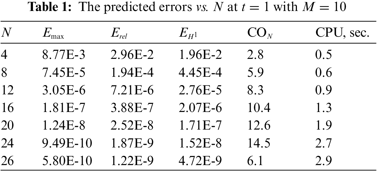
Fig. 2 and Table 2 show the computed
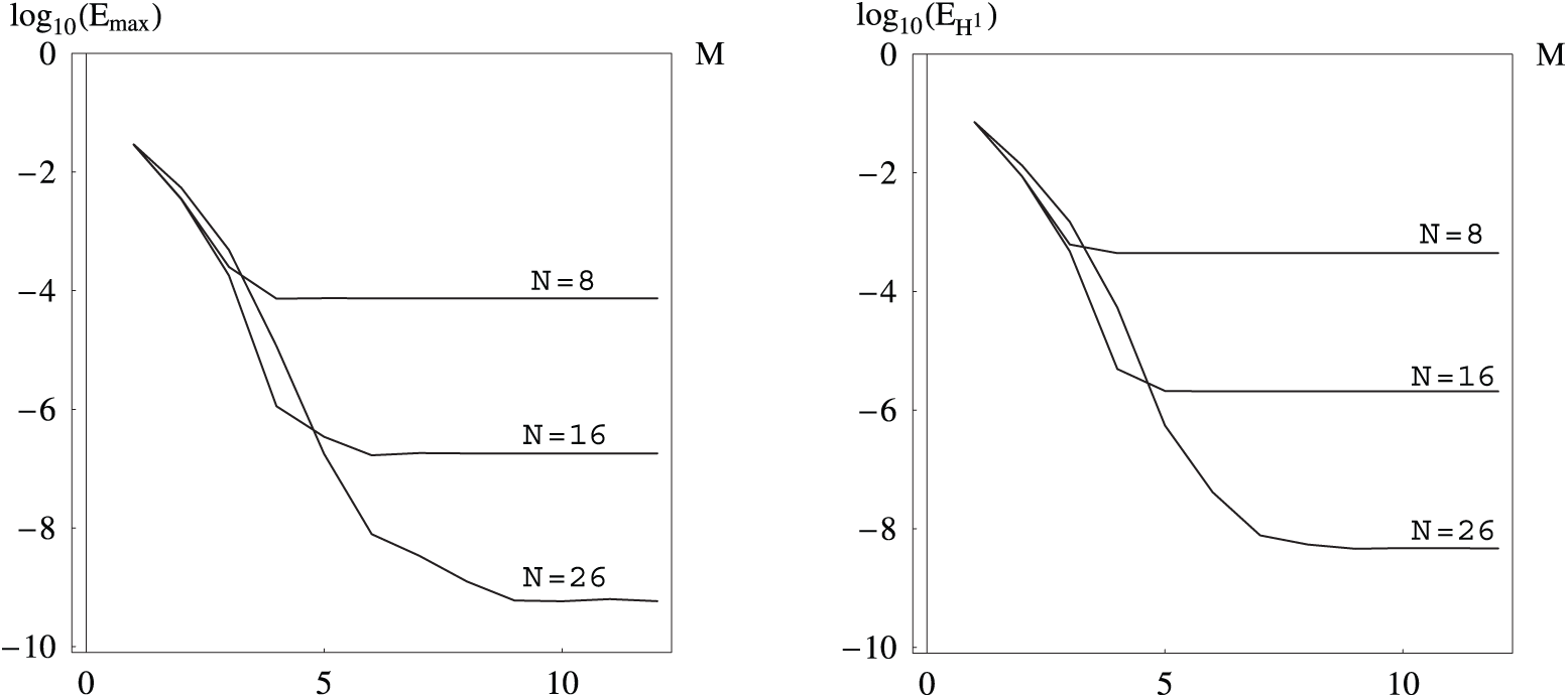
Figure 2: The
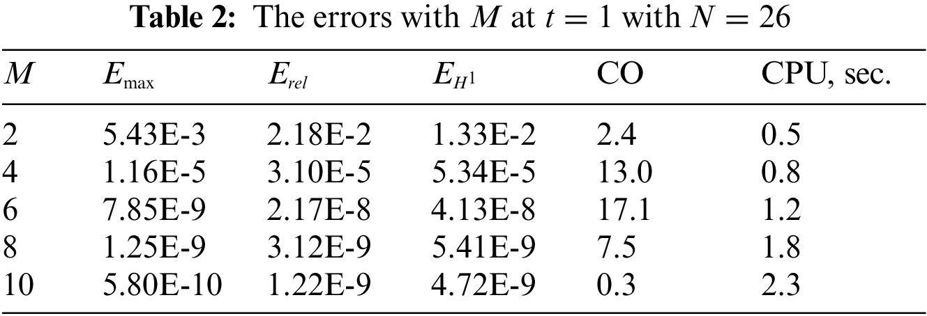

Figure 3: The domain absolute errors with
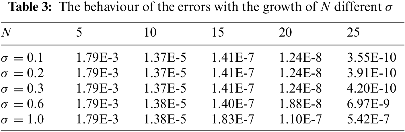
Finally, we show the behaviour of the errors
Let us consider the multi-term problem of the following form:
with the boundary condition of third kind (Robin BCs)
The BCs and IC conform the exact solution
Some results of the calculations are presented in Tables 4 and 5 and displayed in the Figs. 4 and 5. From Tables 4 and 5, we can see that for the problem of the Robin boundary conditions, the proposed method can yield accurate results with small number of basis functions and collocation nodes. And the overall convergence order of the propose scheme is large than two. The same conclusions can be made from Figs. 4 and 5, where the computed maximum absolute errors vs. the M and N are displayed. From these figures, we can see that with the increasing of N for the case


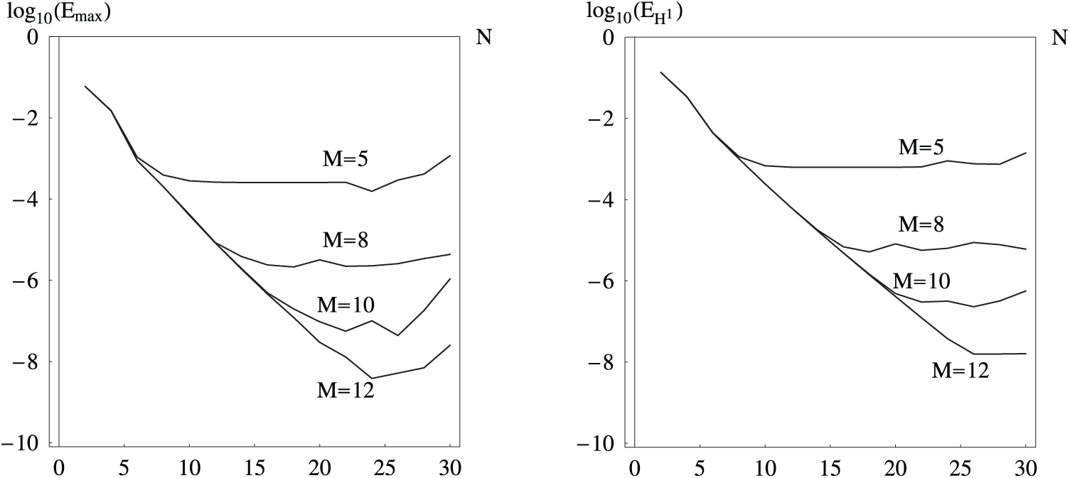
Figure 4: The
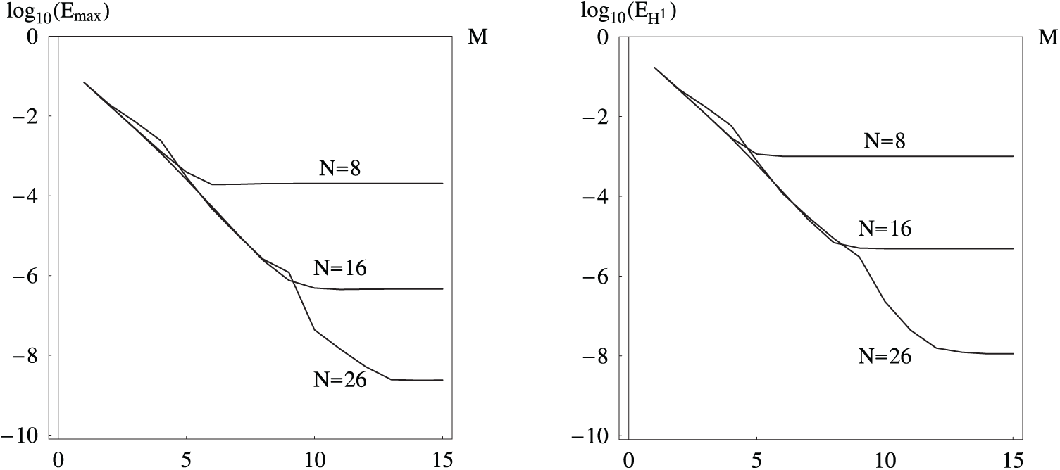
Figure 5: The
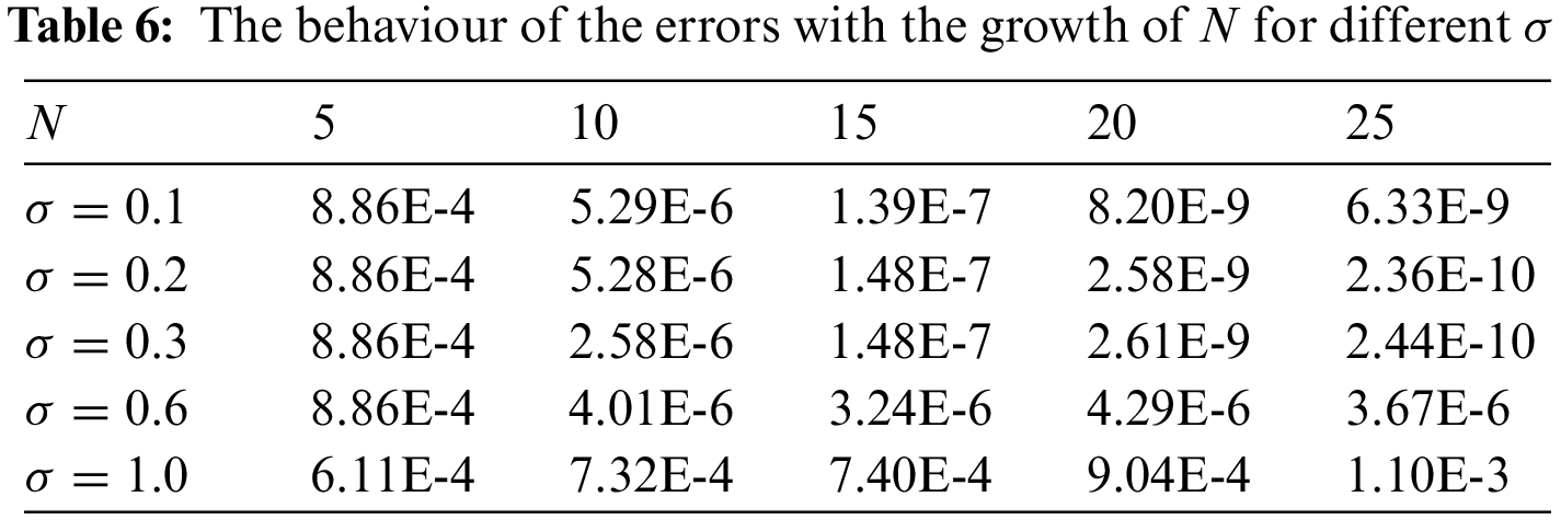
In Table 6, we show the effect of the
Consider the nonlinear time-fractional Huxley equation of the following form:
with
Table 7 and Fig. 6 show the trends of the computed errors with the growth of N with fixed M. The predicted solutions are obtained after 3 iteration of the quasilinearization procedure. The initial approximations of the solution and its derivatives are provided randomly. From the results, we can verify that for the randomly provided initial approximations, we can obtained the accurate solutions in three iterations. And with the increasing of the N, the proposed algorithm converges fast. The same problem was considered by Hadhoud et al. in [41] using a numerical technique based on the cubic B-spline collocation method and the mean value theorem for integrals. The maximal absolute errors obtained there are near


Figure 6: The maximal absolute
Now let us move onto the multi-term nonlinear time-fractional equation with the Huxley nonlinear term,
with the same analytical solution. Here
Fig. 7 demonstrates the behaviour of the errors with the grows of the total amount of basis function
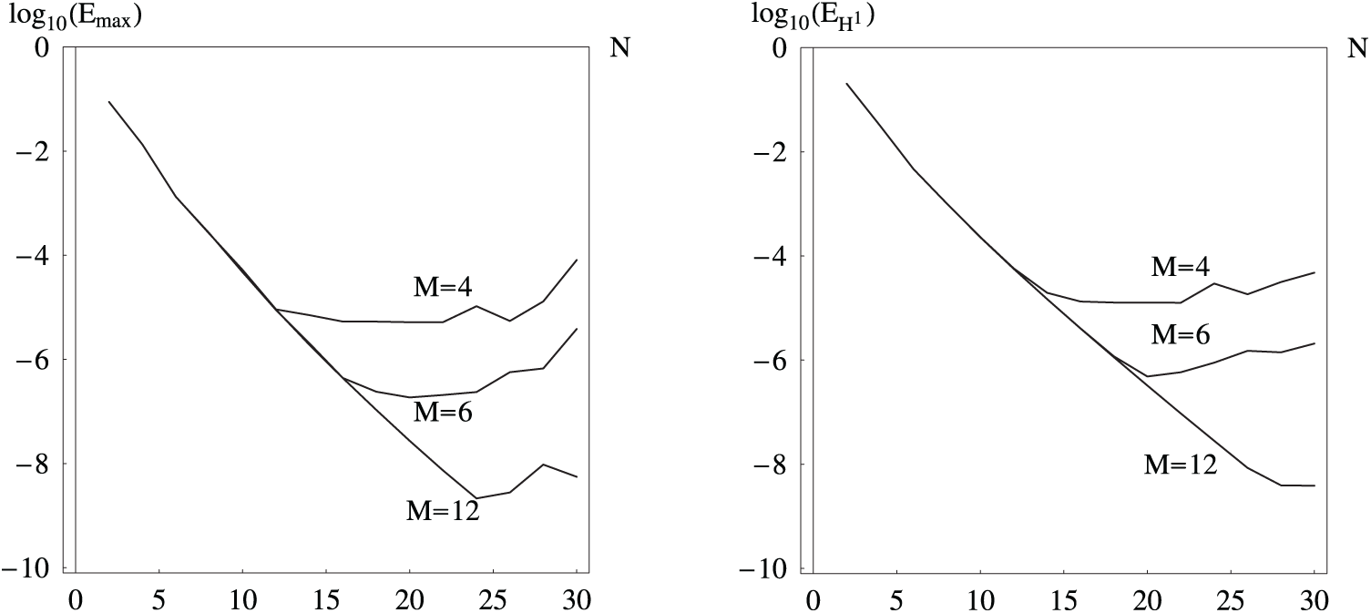
Figure 7: The
Then, we discuss the solution accuracy on the
Let us consider the nonlinear problem with the spatial differential operator of the fourth order
where the spatial operator
and the nonlinear term is
The boundary condition and initial condition conform to the exact
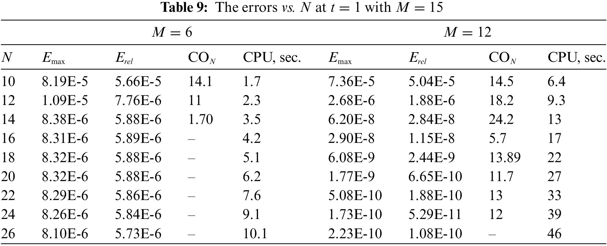
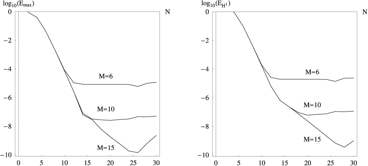
Figure 8: The maximal absolute
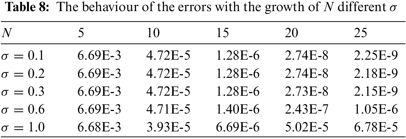
In Table 10, we display the effect of the parameter

4.2 (2+1)-Dimensional Problems
Let us consider the linear fractional equation of the following form:
in the domain governed by
as shown in Fig. 9.

Figure 9: Profile of the irregular domain
Here
where the matrix of diffusivity is
The boundary condition of the Robin type:
and IC conform the exact solution
Table 11 shows the errors as the functions of N where M is fixed at 25, and the maximum error is about

In the last example, we consider a nonlinear problem
in the star-like domain shown in Fig. 10. Here
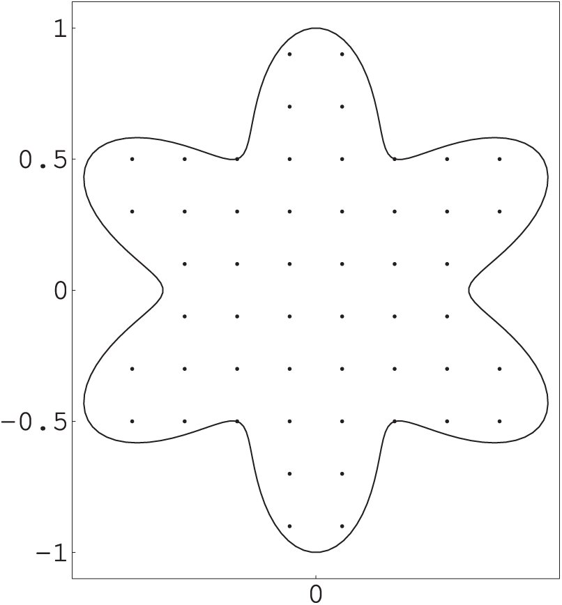
Figure 10: Profile of irregular star-like solution domain
where the matrix of diffusivity is
The Dirichlet boundary conditions and IC can be obtained from
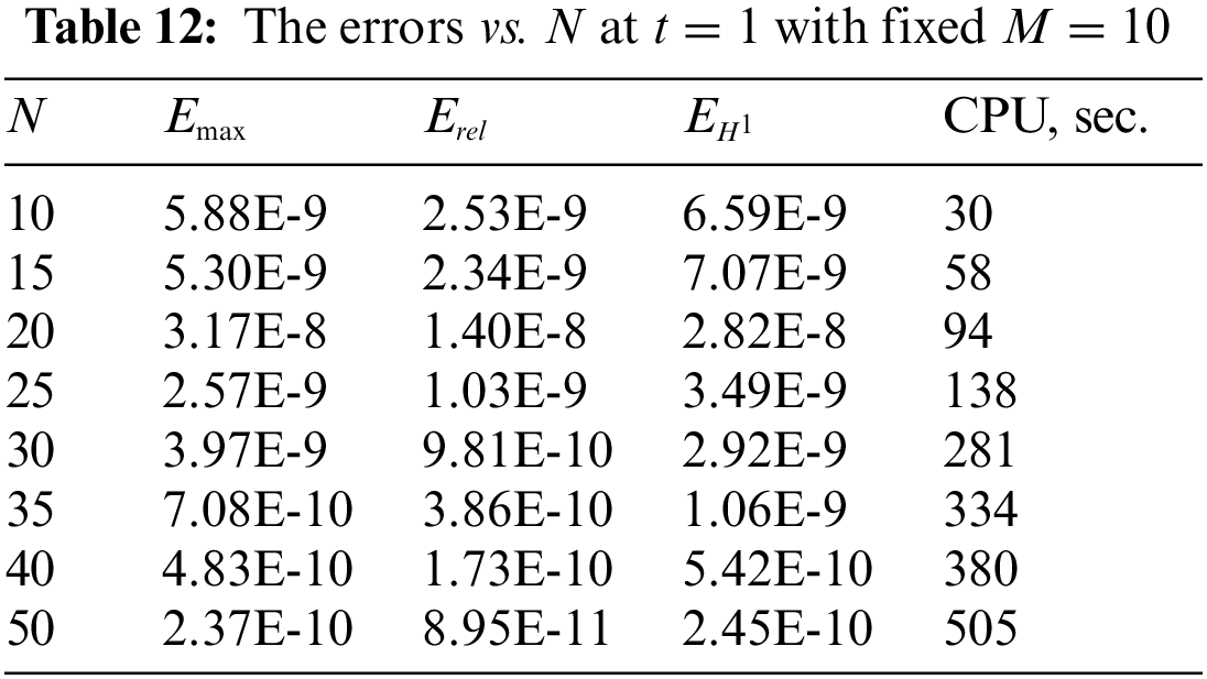
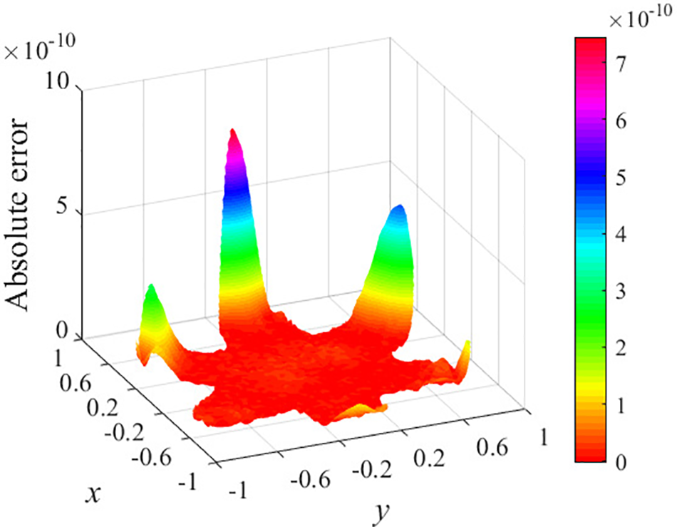
Figure 11: Absolute errors of
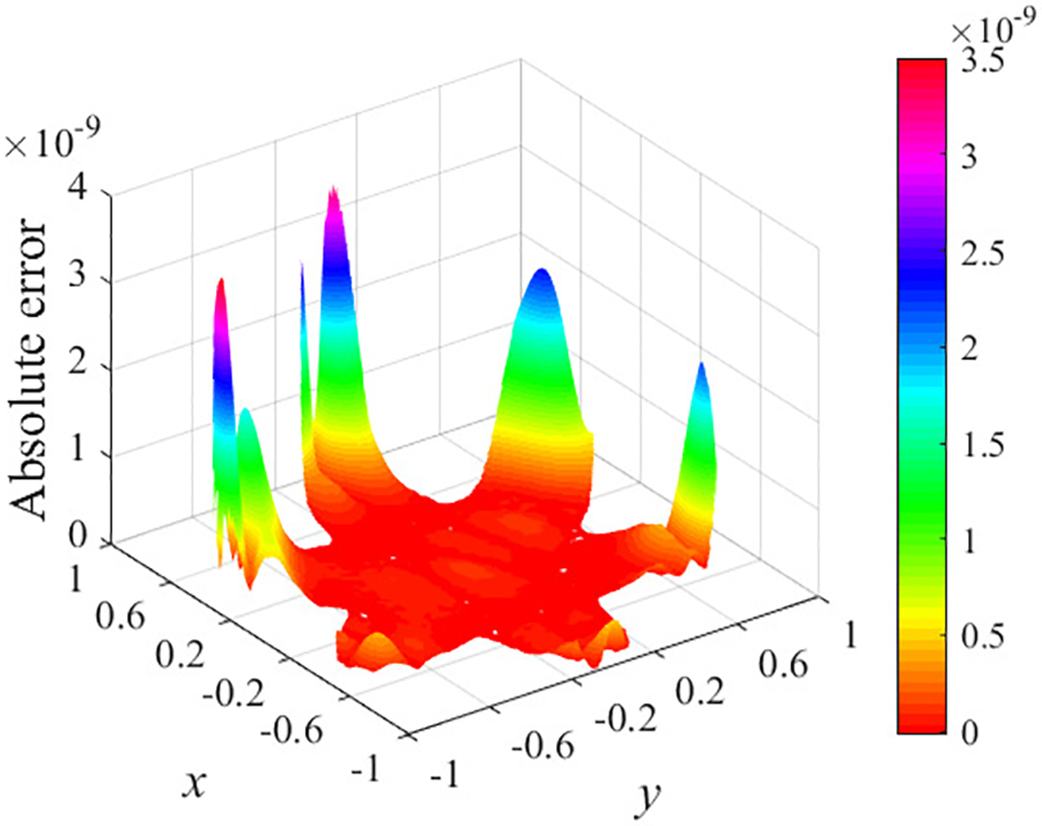
Figure 12: Absolute errors of

Figure 13: Absolute errors of
In order to solve (1+1)-dimensional and (2+1)-dimensional time-fractional nonlinear diffusion equations of multi-term accurately, we propose a simple technique in this paper. First, we convert the original problem into a new one under homogeneous initial conditions by subtracting the initial conditions from the unknown desired solutions. Then the key issue is to solve the problem with zero initial conditions. After that, we try to seek the function
Acknowledgement: The authors wish to express their appreciation to the reviewers for their helpful suggestions which greatly improved the presentation of this paper.
Funding Statement: This research was funded by the National Key Research and Development Program of China (No. 2021YFB2600704), the National Natural Science Foundation of China (No. 52171272), and the Significant Science and Technology Project of the Ministry of Water Resources of China (No. SKS-2022112).
Author Contributions: The authors confirm contribution to the paper as follows: study conception and design: T. Hu, C. Huang, and S. Reutskiy; data collection: J. Lu; analysis and interpretation of results: J. Lin and S. Reutskiy; draft manuscript preparation: J. Lu and J. Lin. All authors reviewed the results and approved the final version of the manuscript.
Availability of Data and Materials: None.
Conflicts of Interest: The authors declare that they have no conflicts of interest to report regarding the present study.
References
1. Liu, L., Feng, L., Xu, Q., Zheng, L., Liu, F. (2020). Flow and heat transfer of generalized Maxwell fluid over a moving plate with distributed order time fractional constitutive models. International Communications in Heat and Mass Transfer, 116(6), 104679. [Google Scholar]
2. Zheng, L., Liu, Y., Zhang, X. (2012). Slip effects on MHD flow of a generalized Oldroyd-B fluid with fractional derivative. Nonlinear Analysis: Real World Applications, 13(2), 513–523. [Google Scholar]
3. Lyu, P., Vong, S. (2019). A high-order method with a temporal nonuniform mesh for a time-fractional benjamin-bona-mahony equation. Journal of Scientific Computing, 80(3), 1607–1628. [Google Scholar]
4. Bayarassou, K. (2021). Fourth-order accurate difference schemes for solving benjamin-bona-mahony-burgers (BBMB) equation. Engineering with Computers, 37(1), 123–138. [Google Scholar]
5. Dehghan, M., Shafieeabyaneh, N., Abbaszadeh, M. (2020). Application of spectral element method for solving sobolev equations with error estimation. Applied Numerical Mathematics, 158, 439–462. [Google Scholar]
6. Zhao, J., Fang, Z., Li, H., Liu, Y. (2020). A crank-nicolson finite volume element method for time fractional sobolev equations on triangular grids. Mathematics, 8(9), 1591. [Google Scholar]
7. Ren, J., Sun, Z. (2015). Efficient numerical solution of the multi-term time fractional diffusion-wave equation. East Asian Journal on Applied Mathematics, 5(1), 1–28. [Google Scholar]
8. Salehi, R. (2017). A meshless point collocation method for 2-D multi-term time fractional diffusion-wave equation. Numerical Algorithms, 74, 1145–1168. [Google Scholar]
9. Yang, X., Qiu, W., Zhang, H., Tang, L. (2021). An efficient alternating direction implicit finite difference scheme for the three-dimensional time-fractional telegraph equation. Computers & Mathematics with Applications, 102, 233–247. [Google Scholar]
10. Shen, S., Liu, F., Anh, V. (2019). The analytical solution and numerical solutions for a two-dimensional multi-term time fractional diffusion and diffusion-wave equation. Journal of Computational and Applied Mathematics, 345, 515–534. [Google Scholar]
11. Stynes, M., O’Riordan, E., Gracia, J. (2017). Error analysis of a finite difference method on graded meshes for a time-fractional diffusion equation. SIAM Journal on Numerical Analysis, 55(2), 1057–1079. [Google Scholar]
12. Soori, Z., Aminataei, A. (2018). Sixth-order non-uniform combined compact difference scheme for multi-term time fractional diffusion-wave equation. Applied Numerical Mathematics, 131, 72–94. [Google Scholar]
13. Jin, B., Lazarov, R., Liu, Y., Zhou, Z. (2015). The Galerkin finite element method for a multi-term time-fractional diffusion equation. Journal of Computational Physics, 281, 825–843. [Google Scholar]
14. Huang, J., Zhang, J., Arshad, S., Tang, Y. (2021). A numerical method for two-dimensional multi-term time-space fractional nonlinear diffusion-wave equations. Applied Numerical Mathematics, 159, 159–173. [Google Scholar]
15. Hussain, M., Haq, S. (2019). Weighted meshless spectral method for the solutions of multi-term time fractional advection-diffusion problems arising in heat and mass transfer. International Journal of Heat and Mass Transfer, 129, 1305–1316. [Google Scholar]
16. Oruç, O., Esen, A., Bulut, F. (2019). A haar wavelet approximation for two-dimensional time fractional reaction-subdiffusion equation. Engineering with Computers, 35(1), 75–86. [Google Scholar]
17. Oruç, O. (2022). An accurate computational method for two-dimensional (2D) fractional Rayleigh-Stokes problem for a heated generalized second grade fluid via linear barycentric interpolation method. Computers & Mathematics with Applications, 118, 130–131. [Google Scholar]
18. Li, J., Dai, L., Nazeer, W. (2020). Numerical solution of multi-term time fractional wave diffusion equation using transform based local meshless method and quadrature. AIMS Mathematics, 5(6), 5813–5839. [Google Scholar]
19. Soltani Sarvestani, F., Heydari, M., Niknam, A., Avazzadeh, Z. (2019). A wavelet approach for the multi-term time fractional diffusion-wave equation. International Journal of Computer Mathematics, 96(3), 640–661. [Google Scholar]
20. Liu, Y., Yin, X., Liu, F., Xin, X., Shen, Y. et al. (2022). An alternating direction implicit legendre spectral method for simulating a 2D multi-term time-fractional Oldroyd-B fluid type diffusion equation. Computers & Mathematics with Applications, 113, 160–173. [Google Scholar]
21. Nikan, O., Tenreiro Machado, J., Golbabai, A. (2021). Numerical solution of time-fractional fourth-order reaction-diffusion model arising in composite environments. Applied Mathematical Modelling, 89, 819–836. [Google Scholar]
22. Zhou, J., Xu, D., Qiu, W., Qiao, L. (2022). An accurate, robust, and efficient weak Galerkin finite element scheme with graded meshes for the time-fractional quasi-linear diffusion equation. Computers & Mathematics with Applications, 124, 188–195. [Google Scholar]
23. Su, B., Jiang, Z. (2020). High-order compact finite volume scheme for the 2D multi-term time fractional sub-diffusion equation. Advances in Difference Equations, 2020, 1–22. [Google Scholar]
24. Ghafoor, A., Khan, N., Hussain, M., Ullah, R. (2022). A hybrid collocation method for the computational study of multi-term time fractional partial differential equations. Computers & Mathematics with Applications, 128, 130–144. [Google Scholar]
25. Piret, C., Hanert, E. (2013). A radial basis functions method for fractional diffusion equations. Journal of Computational Physics, 238, 71–81. [Google Scholar]
26. Hosseini, V., Chen, W., Avazzadeh, Z. (2014). Numerical solution of fractional telegraph equation by using radial basis functions. Engineering Analysis with Boundary Elements, 38, 31–39. [Google Scholar]
27. Liu, Q., Gu, Y., Zhuang, P., Nie, Y. (2011). An implicit RBF meshless approach for time fractional diffusion equations. Computational Mechanics, 48, 1–12. [Google Scholar]
28. Qiao, Y., Zhai, S., Feng, X. (2017). RBF-FD method for the high dimensional time fractional convection-diffusion equation. International Communications in Heat and Mass Transfer, 89, 230–240. [Google Scholar]
29. Reutskiy, S. (2017). A new semi-analytical collocation method for solving multi-term fractional partial differential equations with time variable coefficients. Applied Mathematical Modelling, 45, 238–254. [Google Scholar]
30. Reutskiy, S., Fu, Z. (2018). A semi-analytic method for fractional-order ordinary differential equations: Testing results. Fractional Calculus and Applied Analysis, 21(6), 1598–1618. [Google Scholar]
31. Reutskiy, S., Lin, J. (2018). A semi-analytic collocation method for space fractional parabolic PDE. International Journal of Computer Mathematics, 95(6–7), 1326–1339. [Google Scholar]
32. Lin, J., Zhang, Y., Reutskiy, S. (2021). A semi-analytical method for 1D, 2D and 3D time fractional second order dual-phase-lag model of the heat transfer. Alexandria Engineering Journal, 60(6), 5879–5896. [Google Scholar]
33. Tian, X., Reutskiy, S., Fu, Z. (2022). A novel meshless collocation solver for solving multi-term variable-order time fractional PDEs. Engineering with Computers, 38, 1527–1538. [Google Scholar]
34. Lin, J., Bai, J., Reutskiy, S., Lu, J. (2023). A novel RBF-based meshless method for solving time-fractional transport equations in 2D and 3D arbitrary domains. Engineering with Computers, 39, 1905–1922. [Google Scholar]
35. Pourbabaee, M., Saadatmandi, A. (2022). A new operational matrix based on Müntz-Legendre polynomials for solving distributed order fractional differential equations. Mathematics and Computers in Simulation, 194, 210–235. [Google Scholar]
36. Borwein, P., Erdelyi, T., Zhang, J. (1994). Müntz systems and orthogonal Müntz-Legendre polynomials. Transactions of the American Mathematical Society, 342(2), 523–542. [Google Scholar]
37. Bellman, R., Kalaba, R. (1965). Quasilinearization and nonlinear boundary-value problems. New York, USA: American Elsevier Publishing Company. [Google Scholar]
38. Liu, G., Gu, Y. (2001). A point interpolation method for two-dimensional solids. International Journal for Numerical Methods in Engineering, 50(4), 937–951. [Google Scholar]
39. Liu, G., Gu, Y. (2005). An introduction to meshfree methods and their programming. Berlin, Germany: Springer Science & Business Media. [Google Scholar]
40. Oruç, O. (2023). A strong-form meshfree computational method for plane elastostatic equations of anisotropic functionally graded materials via multiple-scale Pascal polynomials. Engineering Analysis with Boundary Elements, 146, 132–145. [Google Scholar]
41. Hadhoud, A., Abd Alaal, F., Abdelaziz, A., Radwan, T. (2021). Numerical treatment of the generalized time-fractional Huxley-Burgers’ equation and its stability examination. Demonstratio Mathematica, 54(1), 436–451. [Google Scholar]
42. Lin, J., Xu, Y., Zhang, Y. (2020). Simulation of linear and nonlinear advection-diffusion-reaction problems by a novel localized scheme. Applied Mathematics Letters, 99, 106005. [Google Scholar]
Cite This Article
 Copyright © 2024 The Author(s). Published by Tech Science Press.
This work is licensed under a Creative Commons Attribution 4.0 International License , which permits unrestricted use, distribution, and reproduction in any medium, provided the original work is properly cited.
 Downloads
 Citation Tools