Traffic Control Based on Integrated Kalman Filtering and Adaptive Quantized Q-Learning Framework for Internet of Vehicles

1  Introduction

Cities are emerging quickly recently due to the massive development in various fields, such as vehicular communications [1], Internet of Things (IoTs) [2–5], Artificial Intelligence (AI) [6], Fog Computing (FC) [7], as well as smart data analysis and decision making [8]. Several challenges occur in modern cities such as vehicle emissions caused by the transportation systems in general and traffic control [9]. Effective congestion control requires a combination of various technologies, including fast sensor reading and processing, vehicles to vehicles (V2V) and vehicles to infrastructure (V2I) communication, data integration, and intelligent deep learning techniques [10,11]. These technologies can be used to improve congestion control by enabling real-time monitoring and management of traffic flow. For example, V2V and V2I communication can facilitate the exchange of information about traffic conditions, allowing vehicles to adjust their routes and speeds accordingly. Data integration and intelligent deep learning can help to analyze this information and make predictions about future traffic patterns. In addition, decision-making and training of intelligent processes can be used to adapt and improve the performance of the congestion control system [12].

Researchers are interested in developing effective traffic control systems because such systems are key requirements for economic competitiveness and environmental sustainability [10]. Congestion is caused by inefficiencies in traffic regulation, resulting in high expenses and commuter delays. In 2017, the cost of traffic congestion in the European Union (EU) was estimated to be 1% of the yearly GDP. The cost of congestion in the United States was 88 billion dollars in 2019 (0.41% of GDP). Commuters spend up to 200 h a year stuck in traffic, especially in dense cities. Increased emissions as a result of congestion have negative environmental and social consequences [11].

In theory, this should allow for informed control decisions and congestion mitigation. However, traditional traffic control paradigms are inadequate for leveraging the dense stream of state of art to make better control decisions. To deal with the rising complexity of traffic control while taking comprehensive state information into account, new algorithms are required.

Reinforcement learning [12,13] is an artificial learning approach that has proven outstanding results in recent applications of controlling complex systems that have high non-linearity and dynamic nature, such as driverless vehicles [14], unmanned aerial vehicle control [15], and other types of systems which involves sensor reading, data analysis, decision making, and re-training or adaptation. Intelligent traffic control is a suitable example of a highly complex and dynamic system that requires intelligent control and adaptation to external factors [16]. Developing effective RL-based traffic congestion control requires several matters. First, the preparation of communication and sensing infrastructure enables feeding the controller with the state evolution of the environment. Second, developing of estimation algorithm for the state based on the sensing information collected from the sensors. Third, an efficient and effective definition of state that is suitable for different conditions, i.e., an adaptive state. It is observed that the way to handle these issues has not been observed in the existing literature. Therefore, the goal of this article is to address the problem of traffic control from the fourth perspective: Firstly, we propose infrastructure for sensing and communication in a junction combined with our roads. Secondly, we propose a Kalman filtering framework for multi-sensor fusion to obtain an accurate estimate of the state before passing it to the Q-learning. Thirdly, we propose a novel Q-learning formulation combined with state, action, and reward for traffic control over one junction. Fourthly, a comprehensive evaluation of each of the Kalman filters and Q-learning based on eight scenarios of the initial state in the junction and comparing them with the state-of-the-art approaches. This article provides several contributions, as can be stated as follows:

1-   It proposes VANETs infrastructure with IoT-based sensing for enabling communications of vehicles to infrastructure V2I for two functionalities: congestion sensing and smart traffic control. This is distinguished from other articles that ignore sensing and communication infrastructure used to serve traffic congestion control.

2-   It provides an estimation based on multi-sensor Kalman filtering for the state of congestion on the roads in the environment. Kalman filter includes a novel state and measurement models. To the best of our knowledge, this is the first article that incorporates a multi-sensor Kalman filter in the congestion control.

3-   Unlike other Q-learning-based works, it presents an adaptive Q-learning-based traffic control algorithm for roadway types of environments with multi-junction with the adaptive threshold quantitation in order to obtain an adaptive behavior with respect to the change in the density of vehicles.

4-   It evaluates the developed sub-systems, namely, multi-sensor Kalman estimation for traffic congestion estimation and the Q-learning for traffic control using various scenarios in order to provide findings to literature.

The remaining of the article is presented as follows. In Section 2, we present a literature survey about traffic control. In Section 3, an overview Q-learning algorithm is presented. Next, the methodology is presented in Section 3. Afterward, experimental results are presented in Section 4. Lastly, the conclusion and future works are presented in Section 5.

2  Literature Survey

Traffic congestion has been examined widely in the literature. Some approaches have focused on modeling traffic flow. In the work of Isaac et al. [17], the prediction and modeling of traffic flow of human-driven vehicles at a signalized road intersection using an artificial neural network model was proposed. The evidence from this study suggests that the ANN predictive approach proposed could be used to predict and analyze traffic flow with a relatively high level of accuracy. Another significant evidence from this study suggests that the ANN model is an appropriate predictive model for modeling vehicular traffic flow at a signalized road intersection. In the work of Kang et al. [18], the viscoelastic traffic flow model was simplified. The fractional viscoelastic traffic flow model is established in combination with modeling principle of the Bass model and the successful application of fractional calculus in viscoelastic fluid. Conformable fractional derivative and the fractional grey model are then introduced to establish a fractional grey viscoelastic traffic flow model that can reflect time-varying characteristics. Finally, the new model is compared with traditional statistical models in terms of model efficiency and stability and is applied to the modeling of traffic flow and traffic congestion levels in multiple scenarios. Other researchers have leveraged deep learning models including Convolutional Neural Network (CNN), Recurrent Neural Network (RNN), Long Short-Term Memory (LSTM), Restricted Boltzmann Machines (RBM), and Stacked Auto Encoder (SAE) [19]. In the work of Olayode et al. [20], traffic flow variables, such as the speed of vehicles on the road, the number of different categories of vehicles, traffic density, time, and traffic volumes, were considered input and output variables for modeling traffic flow of non-autonomous vehicles at a signalized road intersection using the artificial neural network by particle swarm optimization (ANN-PSO). Other works have concentrated on traffic congestion prediction [21].

Various approaches have focused on various aspects, such as delay estimation proposed by Afrin et al. [22]. Rani et al. [23] proposed an approach for traffic delay estimation considering technical and non-technical factors. The approach was based on a fuzzy inference system, which is criticized by the need for an exhausting tuning process. Another aspect is traffic detection and estimation. Zhang et al. [24] proposed a road traffic detection system that uses RFID-based active vehicle positioning and vehicular ad-hoc networks (VANETs) to detect traffic congestion dynamically was proposed. The estimation is based on various variables, namely, vehicle density, weighted average speed and congestion level. Chaurasia et al. [25] used a combination of data mining historical trajectory data to detect and predict traffic congestion and VANET in reducing the detected congestion events. The trajectories are firstly pre-processed before they are clustered. Congestion detection is then done for each cluster based on a certain speed threshold and the time duration of that particular event. The problem of traffic control was tackled recently and several models were developed for addressing it under several categories.

The category of reinforcement learning-based traffic control was the most effective one proposed by Wu et al. [26]. Joo et al. [27] used a traffic signal control (TSC) system to maximize the number of vehicles crossing an intersection and balances the signals between roads by using Q-learning (QL). States are determined by the number of directions on the road. There are only three action sets available. When an action set is selected, only the direction of the road corresponding to that action will have a green light. To minimize the delay in an intersection, the reward function is configured with two parameters, i.e., the standard deviation of the queue lengths of the directions and throughput. Busch et al. [11] proposed representative Deep Reinforcement Learning (DRL) agents that learn the control of multiple traffic lights without and with current traffic state information. The agnostic agent considers the current phase of all traffic lights and the expired times since the last change. In addition, the holistic agent considers the positions and velocities of the vehicles approaching the intersections. In [28], Q-learning was applied to reduce the congestion based on traffic control. In their formulation of Q-learning, four types of actions were defined with preserving one of the traffic lights at the junction fixed and enabling the other one to increase or decrease by ∓5. The reward function used an average vehicle delay time. In [29], a semi-cooperative Nash Q-learning and an extended Stackelberg equilibrium Q-learning were proposed. Instead of adjusting the plan of green light timing, they determined the best multi-routes plan for passing most vehicles in a single traffic intersection, combining game theory and RL in decision-making in the multi-agent framework. In [30], an RL-based cooperative traffic signal control scheme considering the data transmission delay issue in a traffic road network was proposed. four traffic features to describe the traffic states of an arbitrary intersection. Four features are used to describe the state, namely, local current traffic signal, phase, vehicle volumes, average speed, and average acceleration. The action space uses two actions for left turn permitted and four actions for left turn protected. The reward is calculated using the pressure on the intersection. In [31], Reinforcement Learning (RL)-based variable speed limits (VSL) control algorithm was proposed to reduce crash risks associated with oscillations. The state, action and reward, which are the critical components in the RL, were designed carefully for safety improvement. The RL was trained to learn the optimal speed limit for various traffic states to achieve the goal of safety optimization. A rear-end crash risk model was applied to assess crash risks associated with oscillations near freeway bottlenecks. The cell transmission model was modified as the simulation platform for evaluating the control effects. density within the three sections is used to be the state set. The action was used to set the speed limit. The reward was described based on the total crash risk (TCR) over a time horizon.

The usage of the Kalman filter for smart city applications has been observed in the literature. In [32], the Kalman filter is used for anomaly detection based on a fisheye camera and image processing. In [33], the Unscented Kalman filter has been applied in traffic control benchmarking for comparison with the observer framework for performing the traffic density estimation. In [34], the cubature Kalman filter algorithm is used as part of an algorithm for estimating estimate vehicle information and real-time road conditions, whilst fuzzy logic is used to correct the measurement noise of the Kalman filter. The ant colony algorithm is used to optimize the input and output membership functions. In [35], a 15-state Kalman Filter was developed for a navigation system based on two smart phones’ IMU sensors, “Xiaomi 8” and “Honor Play”. Their results have shown that the navigation solutions of both smartphones are quite close to that of the reference IMUs. We present a summary of the existing algorithms for traffic prediction and control with their limitation in Table 1. Two aspects are mentioned in the table, namely, traffic prediction and traffic control. As is shown, none of the existing algorithms have combined the two aspects jointly in the table.

Overall, the two problems of traffic estimation and traffic control were addressed separately in the literature, despite the relationship between them. The literature did not jointly address them. The benefit of integrated traffic estimation and traffic control is exploiting the inter-effect to increase the performance of each of them. Developing such a solution requires defining a sufficient state to link traffic estimation and traffic control on one side and an effective reward to create feedback from the traffic control into the estimation.

In this article, we presented a unified framework for handling the two problems together. Firstly, an infrastructure based on IoT sensing and two types of communication, namely, V2V and V2I, are presented. Secondly, an estimation based on multi-sensor Kalman filtering for the state of congestion on the roads in the environment is provided. Thirdly, a learning-based traffic control algorithm for roadway types of environments with multi-junction is proposed. Lastly, the article evaluates the developed sub-systems, namely, the multi-Kalman estimation for traffic congestion estimation and the Q-learning for traffic control using various scenarios with a comparison with the state-of-the-art approaches.

3  Methodology

This section presents the developed methodology of this article. It starts with formulation of the traffic control. Next, we present an overview of Q-learning. Afterward, we present the communication infrastructure and system architecture. Next, a mathematical model and reinforcement learning are presented. Next, we present a vehicle generation model, driving behavior model, mobility variables, and lane change model. Lastly, we present the evaluation metrics.

3.1 Formulation of the Traffic Control Problem

The problem we are solving is traffic congestion control. It is handled in MATLAB simulation. The problem is formulated mathematically as follows. Given an urban environment combined with multiple junctions where each junction indicates an intersection between horizontal and vertical lines. Each line is a combination of set roads with two directions and each direction has multiple lanes. The vehicle generation is appled to all roads at their intersection with the border of the environment for the IN direction and the vehicles leaving is applied to all roads at their intersection with the border of the environment in the OUT direction. Each junction has two modes, namely, road centered and junction centered.

In the former, the action enables at one time east and west (EW) or north and south (NS). In the latter, the action enables opening one of the four roads (E, W, N, and S) to three directions corresponding to the enabled road: forward, right, and left. The state transition diagram of each of the two modes is depicted in Fig. 1. It is observed that the system follows a Markov decision process (MDP). In any current state, the transition to the next state depends only on the current state and it does not have a relation with the previous states. We assume that each road is occupied with load cells at its two ends for measuring the flows of vehicles and cameras to measure the count of the vehicles. Furthermore, the vehicles are occupied with IEEE 802.11p for communicating with other vehicles and with roadside units available at each junction. Assuming that the vehicles are generated using normal distribution probability density function for several vehicles and exponential distribution probability density function for time interval and assuming that the two types of sensors are subject to noise, our goal is to exploit the sensing, V2V and V2I communication for enabling two functionality states estimation using sensor fusion and traffic control using reinforcement learning.

Figure 1: Markov process of traffic control for traffic control-a-junction centered mode-b-road centered mode

Six types of traffic opening are used:

•   North–South (N–S): The traffic sign of the southern and eastern roads is open while the remaining signs are closed

•   East–West (E–W): The traffic sign of the eastern and western roads is open while the remaining signs are closed

•   S: The traffic sign on the southern road is open while the remaining is closed

•   N: The traffic sign on the northern road is open while the remaining is closed

•   E: The traffic sign on the eastern road is open while the remaining is closed

•   W: The traffic sign on the western road is open while the remaining is closed

3.2 Overview of Q-Learning

A fundamental algorithm developed in the literature is used in building our traffic control algorithm, namely, the Q-learning algorithm. As presented in Fig. 2, it takes the states, actions, rewarding function R, the transition function T, the learning rate Alpha, and the discount factor Gamma. The output of the algorithm is the Q matrix. The algorithm starts with initiating the Q matrix based on the number of actions and the number of states. The algorithm starts with a set of episodes until reaching convergence when the Q matrix does not change anymore. In each episode, the algorithm determines the best action according to the Q matrix, it activates the action using the transition matrix and it finds the next state, it also uses the reward function to find the reward, and it uses the Bellman equation to update the Q matrix based on learning rate α and discount factor γ. Hence, the algorithm works by learning an action-value function Q(st,at), which estimates the expected reward an agent will receive by acting a in state st. The Q function is updated based on the agent’s experiences in the environment using the following Eq. (1):

Q(st,at)=Q(st,at)+α(rt+γmax(Q(st+1,at+1)−Q(st,at)))(1)

where

st denotes current state

at denotes current action

st+1 denotes next state

at+1 denotes next action

α denotes the learning rate

γ denotes discount factor, the discount factor determines the importance of future rewards and is a value between 0 and 1.

Figure 2: Flowchart of Q-learning algorithm

3.3 Flowchart of Development

It starts with sensing and communication architecture. Next, a development of sensor fusion for state prediction using Kalman filter is provided with novel process and measurement model for Kalman filter. Afterward, the development of Q-learning agent using state, action, and reward is presented. Lastly, the training of the agent and evaluation of the decision making is given. A conceptual diagram of the four types of communications is depicted in Fig. 3.

Figure 3: Conceptual diagram of the developed methodology in the article

3.3.1 Communication Infrastructure

The communication infrastructure represents the various types of communications which exist in the urban environment. There are four types of communication:

•   Traffic light to Traffic light (T2T): it is responsible for enabling negotiation between two junctions to mitigate the congestion which emerges at two adjacent junctions.

•   Vehicles to Traffic light (V2T): it is responsible for enabling negotiation between certain vehicles associated with the urgent condition or state with its traffic light.

•   Vehicle to Base station (V2B): it is responsible for providing emergency messages from the vehicle to the Road Side Unit (RSU) in the case of an emergency.

•   Vehicle to Vehicle (V2V): it is responsible for data dissemination under multi-hop topology when an emergency occurs at one vehicle which has no direct connectivity with the roadside unit or traffic.

3.3.2 System Architecture

The proposed traffic control system is depicted in Fig. 4. As shown in the figure, the inputs of the system are the IoT sensors and the vehicle information that provides data to the base station. IoT sensors are responsible for providing information on vehicle counts on each lane while vehicle information provides ID of vehicle. The base station contains two distinct components: the first one is the sensor fusion using Kalman filtering and the second one is the agent of reinforcement learning which uses the states estimated by the Kalman filter for providing the actions of traffic control.

Figure 4: The system architecture for traffic control using Kalman filtering and reinforcement learning

The actions are transmitted to traffic signals for controlling the various traffic signals that have been provided in the problem formulation. The actions are associated with the four segments of the road, namely, east E, west W, south S, and north N. There are two types of set of actions: (1) road-centered which activates green light for one of the four segments at one time and allows traffic to go through, turn right, and turn left. (2) junction-centered which activates green light for two of four segments at one time either for north and south or for east and west. It also allows for left direction only.

3.3.3 Mathematical Model

The role of the sensor fusion is to estimate the state of traffic at each road at the end direction associated with the junction. Assuming that the junction is Junij where i indicates the horizontal road of the junction and j indicate the vertical road of the junction. For the junction Junij, we have four roads belonging to the set of R(Junij)={Nj,Sj,Ei,Wi} and eight directions belonging to the set.

Dir(Junij)={NjN,SjN,EiE,WiE,NjS,SjS,EiW,WiW}(2)

The state that is estimated by using the information filter is

x=[C(NjN),C(SjN),C(EiE),C(WiE),C(NjS),C(SjS),C(EiW),C(WiW)]T(3)

where

C(d) denotes the vehicles count in direction d.

The process model is described by Eq. (4).

xt=Axt−1+But(4)

u denotes the input of the process model and it is updated from the sensors of weight cells that are located at the inputs and outputs of the roads to the junction.

C(NjN)t=C(NjN)t−1+Win(NjN)t− Wout (NjN)t(5)

C(SjN)t=C(SjN)t−1+Win(SjN)t− Wout (SjN)t(6)

C(EiE)t=C(EiE)t−1+Win(SiE)t− Wout (SiE)t(7)

C(WiE)t=C(WiE)t−1+Win(WiE)t− Wout (WiE)t(8)

C(NjS)t=C(NjS)t−1+Win(NjS)t− Wout (NjS)t(9)

C(SjS)t=C(SjS)t−1+Win(SjS)t− Wout (SjS)t(10)

C(EiW)t=C(EiW)t−1+Win(SiW)t− Wout (SiW)t(11)

C(WiW)t=C(WiW)t−1+Win(WiW)t− Wout (WiW)t(12)

ut=[WinC(NjN),WinC(SjN),WinC(EiE),WinC(WiE),WinC(NjS),WinC(SjS),Win(EiW),Win(WiW),WoutC(NjN),WoutC(SjN),WoutC(EiE),WoutC(WiE),WoutC(NjS),WoutC(SjS),WoutC(EiW),WoutC(WiW)]tT(13)

A=I8×8(14)

B=(10000000−10000000010000000−10000000010000000−10000000010000000−10000000010000000−10000000010000000−10000000010000000−10000000010000000−1)(15)

xt=Hizt(16)

zt=x=[CA(NjN),CA(SjN),CA(EiE),CA(WiE),CA(NjS),CA(SjS),CA(EiW),CA(WiW)]T(17)

where

CA(d) denotes the camera reading of vehicles count in direction d.

H=(1000000001000000001000000001000000001000000001000000001000000001)(18)

The state is predicted by the process model, which is combined with two terms: the transition term Ax^(t∣t) and the input term Bu(t).

x^(t+1∣t)=Ax^(t∣t)+Bu(t)(19)

After predicting the state based on the process model, we predict the covariance matrix P based on the Eq. (20).

P(t+1∣t)=AP(t∣t)AT+Q(20)

where

Q=σQI8×8

σQ is an indicator to the non-confidence in the process model.

Next, we corrected the state using Eqs. (21) and (22).

x^(t∣t)=x^(t∣t−1)+∑i=1Nii(t)(21)

ii(t)=HiTRi(t)−1zi(t)(22)

where

Ri(t)=σR,iI8×8

σR,i is an indicator to the non-confidence in the measurement model.

x^(t∣t)=&P(t∣t)P(t∣t−1)−1x^(t∣t−1)+∑i=1NP(t∣t)HiTRi(t)−1zi(t)(23)

P(t∣t)=(P(t∣t−1)−1+∑i=1NHiTRi(t)−1Hi)−1(24)

3.3.4 Reinforcement Learning

The algorithm of reinforcement learning-based traffic control is defined based on the elements of the RL systems, namely, agent, state, action, reward, and Q-matrix [36]. We present them as follows:

1.    Agent: is a process that runs at the base station and it is responsible for relying on the state provided by the information filter to give the needed decision according to the learned knowledge represented by the policy function.

2.    Actions: are defined based on the control signal that enables the switching of the traffic signs between the various modes. We define for the junction two modes: junction centered (left-protected) and road centered (left-permitted). For the former, we have two corresponding actions: {N−S,E−W} and, for the latter, we have four corresponding actions {E,W,N,S}. Hence, the overall set of actions is A={N−S,E−W,E,W,N,S}.

3.    States: are defined based on the quantization of the roads to two levels low L and high H. Considering that we have four roads {E,W,N,S} and we have for each road two levels, then the state is a vector described by the values of its roads. In total, we have 24=16 states. For quantization of state to L which indicates low congestion and H which indicates high congestion, we used an adaptive threshold. The adaptive threshold is calculated based on the highest congestion road at the time of calculation at the junction according to Eq. (25).

AT=max(NR(Junction))−CMR(25)

where

AT denotes the adaptive threshold

NR denotes the number of vehicles in the subject junction and it is equivalent to NR=[N1N2N3N4], where Ni indicates to the number of vehicles on the road i.

CMR denotes the congestion minimum range

4.   Reward: it represents the shaping function of the action and it is calculated based on the average waiting time of vehicles in the network which needs to be minimized.

5.   Q-matrix is a 2D matrix combined of 16 rows and six actions. It contains a total number of 96 elements.

3.3.5 Traffic Modeling

This section presents sub-models used in our development. First, the vehicle generation model is provided. Second, driving behavior model is presented. Third, we provide driving behavior model. Fourth, we present the mobility variables. Lastly, the lane change model is given.

A- Vehicles generation model

We assume that the vehicles are generated in the environment from certain points we name them as inflow points. At each inflow point, the vehicles are generated based on batches. B={Bt1,Bt2,…Bt,…} where each batch Bti is generated at certain point of time t(i)

t(i)−t(i−1)=T(26)

Also

|Bt(i)|=N(27)

where

T∼exponential pdf with parameter λ

N∼normal pdf with parameter μ and σ.

B- Driving behavior model

The velocity is calculated as an integration of the acceleration with limiting it with the minimum and maximum velocity. The minimum velocity is assumed to be Vmin=0 because we allow vehicles to stop in the urban environment.

The maximum velocity is assumed to be Vmax, which is one of the properties of the segment of the road where the vehicle is moving. The concept of acceleration integration is given in Eq. (28).

vi(t+Δt)={min(vi(t)+ai(t)Δt,Vmax) if ai(t)≥0max(vi(t)+ai(t)Δt,Vmin) if ai(t)<0(28)

However, the vehicles will not receive a fixed acceleration because drivers change their behavior in terms of deceleration or acceleration. The model of calculating the acceleration is provided in Eqs. (29) to (31).

ai(t)={R2Amax R2(−1)Dmax, 0,  if R1<acci+prif acci+pr<R1R1<acci+dacci+2protherwise(29)

acci={R4(1−2pr),ifR3<3AGG40,otherwise (30)

dacci={R4(1−2pr),if 3AGG4<R3<AGG0,otherwise (31)

where

R1, R2, R3 and R4 represent random numbers between 0 and 1 generated uniformly

pr is a controlling parameter

AGG denotes the aggressiveness

Amax and Dmax denotes the maximum and minimum values of the acceleration and deceleration, respectively.

C- The mobility variables

The velocity is calculated as an integration of the acceleration with limiting it with the minimum and maximum velocity. The minimum velocity is assumed to be Vmin=0, because we allow vehicles to stop at the urban environment. The maximum velocity is assumed to be Vmax , which is one of the properties of the segment of road where the vehicle is moving. The concept of acceleration integration is given in Eq. (31).

vi(t+Δt)={min(vi(t)+ai(t)Δt,Vmax) if ai(t)≥0max(vi(t)+ai(t)Δt,Vmin) if ai(t)<0(32)

However, the vehicles will not receive a fixed acceleration because drivers change their behavior in terms of deceleration or accelerating. The model of calculating the acceleration is provided in Eqs. (33) to (35).

ai(t)={R2Amax,if R1<acci+prR2(−1)Dmax,if acci+pr<R1<acci+dacci+2pr0,otherwise(33)

acci={R4(1−2pr),if R3<3AGG40,otherwise (34)

dacci={R4(1−2pr),if 3AGG4<R3<AGG0,otherwise (35)

where

R1, R2, R3 and R4 represents random numbers between 0 and 1 generated uniformly.

pr is a controlling parameter.

AGG denotes the aggressiveness.

Amax and Dmax denotes the maximum and minimum values of the acceleration and deceleration, respectively.

D- Lane change model

As shown in Fig. 5, we assume that drivers tend to keep their driving in the same lane. However, there is a probability of lane changes according to the distance between the subject vehicle and the vehicle ahead and the relative velocity between them. Furthermore, the two ahead vehicles are in the adjacent lanes.

Figure 5: Algorithm for simulating lane change in the mobility model used in Talib et al. [37]

The model of lane changing assumes that the vehicles do lane changing under two probabilities pn or pu. The first one indicates a normal situation, while the second one indicates an urgent situation, which is one the vehicle ahead is close to the subject vehicle. In both cases: the vehicle does not change lanes until assuring that the target lane is available.

3.4 Evaluation Metrics

For evaluating our approach, we use three evaluation metrics, namely, the estimation error of has the role of evaluating the estimation, the average waiting time, and the number of released vehicles, which are responsible for measuring the performance of the traffic control.

The evaluation will use the following metrics:

3.4.1 Error

The estimation error for each road R is ER and it represents the difference in the number of vehicles between the true ones and the estimated ones by the Kalman Filtering approach. This metric needs to be minimized.

ER=|NR−N~R|(36)

where

NR denotes the number of vehicles on the road R.

N~R denotes the estimated nu

3.4.2 Average Waiting Time

It represents the average waiting time of the vehicles on the road of the junction before they are released.

AWT=∑i=1NRWTiNR(37)

where

WTi denotes the waiting time of vehicle i on the road R

The above section presents the development methodology of our sensor fusion RL based traffic control. It consists of Q-Learning Algorithm that is presented in Sub-Section 3.1, the formulation of the traffic control problem that is presented in Sub-Section 3.2. Next, we provide the communication infrastructure in Sub-Section 3.3. Afterward, we provide the sensor fusion in Sub-Section 3.4.

4  Experimental Results and Evaluation

This section provides the experimental design and the analysis and evaluation. It comprises two subsections: the experimental design which presents the parameters of the developed algorithm and the experimental results and analysis which is given in Section 4.2.

4.1 Experimental Design Waiting Time

For evaluation, MATLAB 2020a environment was used for implementing the simulation. we use the parameters presented in Table 2. The action duration is set to 10 s, the number of iterations is set to 30 s. The Kalman filtering parameters are the initial variance σP2 which is set to 100, the process variance σQ2 and it is set to 0.1, and the measurement variance σR2 which is set to 0.5. The chosen parameters for the traffic congestion control system strike a balance between responsiveness, computational efficiency, and handling uncertainties. A 10-second action duration enables timely responses and smooth traffic flow, while 30 iterations allow the RL model to learn and adapt efficiently. The initial variance (σP2 = 100) accounts for the uncertainty in the initial state estimate, enabling quick adaptation. The process variance (σQ2 = 0.1) indicates stable and predictable system dynamics, suitable for typical traffic patterns. However, adjustments may be required for more complex scenarios. Lastly, the measurement variance (σR2 = 0.5) acknowledges noise in measurements from sensors and cameras, allowing the Kalman filter to better filter out noise and enhance state estimate accuracy.

The parameters of the simulation environment are given in Table 3. As presented earlier, the environment represents an intersection area comprising four roads, R1, R2,R3 and R4. The lengths are 1500 m for R1 and R2, and 3000 m for R3 and R4. The aggressiveness factor was set to 0.8, the probability of lane change was set to 0.5 for normal situation lane change pn and 0.9 for urgent case lane change  pu. The relative distance threshold for urgent lane change is set to DistRelT, which is equivalent to 10.

For evaluation, we have considered ten scenarios which are classified according to the initial state of vehicles on the roads of the junction and to the incoming vehicle numbers. As depicted in Table 4, scenario 1 is associated with an initial high number of vehicles for R2,R3 and R4 and a low number of vehicles for R1, and low incoming vehicles. The intersection contains four roads. We simulated eight scenarios of three congested roads and one non-congested and two scenarios of four congested roads. Each of the two scenarios corresponds to a low and a high incoming vehicle rate. Hence, the total number of scenarios is ten.

4.2 Experimental Results

This section presents the evaluation of our developed approach. It comprises two subsections, the traffic control evaluation is presented in Sub-Section 4.2.1 and the Kalman filtering approach is presented in 4.2.2.

4.2.1 Traffic Control Evaluation

For evaluation, we compared our developed approach in [27], which uses also a Q-learning approach with a standard deviation term in the reward function. We use the suffix STD with the label of this approach or Q-STD. In addition, we used greedy-based traffic control as another benchmark and it is labelled as greedy. The meaning of greedy indicates the greedy behavior of giving priority to the most congested road at the moment of decision making.

We are interested in two metrics, the first one of which is the average waiting time presented in Fig. 6. It shows that Q-STD has accomplished the least average waiting time compared with greedy and AQQL. However, AQQL was superior to greedy in terms of the average waiting time. AQQL has accomplished a higher number of released vehicles, as shown in Fig. 7, which meant superiority over both greedy and Q-STD. The number of released vehicles is more transparent about the performance than the average waiting time, considering that the latter is only calculated based on the vehicles that have been released.

Figure 6: The average waiting time for Q-learning, Q-learning STD and greedy

Figure 7: Number of released vehicles for Q-learning, Q-learning STD and greedy

Another observation is that Q-STD, which has accomplished the least average time, is not capable of maintaining the number of vehicles on the road lower than the permitted threshold, which indicates the road capacity. This is visualized from the graphs in Fig. 8, which shows a continuous increase in the number of vehicles on the roads, indicating that the average waiting time is not an indicator of good performance because it is only calculated for a small portion of the vehicles or the vehicles which were released from the road after waiting. This is more obvious in scenario 2 where the number of vehicles on the road had increased to beyond 400 vehicles, which caused failure in the approach compared with Q-learning. The number of 400 was taken as a threshold of failure based on the assumed dimension of the road in the simulation scenarios.

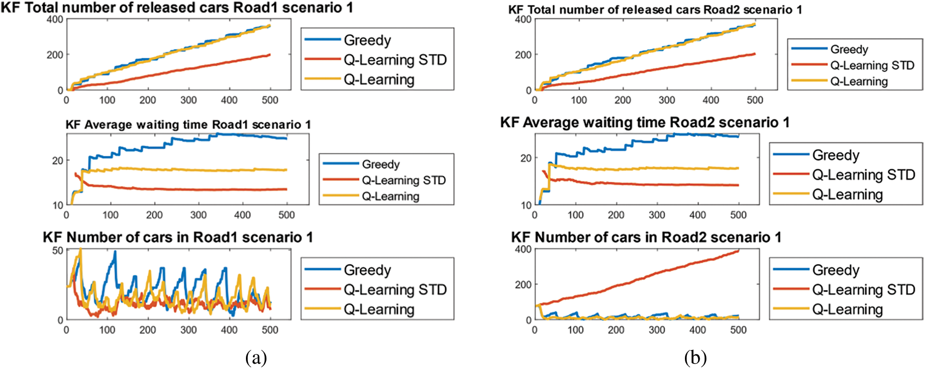
Figure 8: Time series of the metrics for the four roads of scenario 1-a-Road 1-b-Road 2-c-Road 3-d-Road 4

The time-series results of scenarios 1, 2, and 3 based on Kalman filter are presented in Figs. 8–10, respectively. As we observed for scenario 2, the number of released vehicles increased for both greedy and AQQL while it suddenly went to zero for AQQL. This is interpreted by the failure of Q-STD in managing the intersection due to exceeding the number of vehicles or vehicles beyond the capacity of the road. As mentioned earlier, the number of 400 was taken as a threshold of failure. This has been observed in road 2. For comparing AQQL and greedy, we observed that the average waiting time was higher for greedy than AQQL for all roads with a higher number of released vehicles.

Figure 9: Time series of the metrics for the four roads of scenario 2-a-Road 1-b-Road 2-c-Road 3-d-Road 4

Figure 10: Time series of the metrics for the four roads of scenario 3-a-Road 1-b-Road 2-c-Road 3-d-Road 4

4.2.2 Kalman Filtering Perspective

The evaluation of the performance from the perspective of Kalman filter is presented in Fig. 11. The Kalman filter developed in this article is denoted by multi-sensor Kalman filter and it will be compared with the traditional Kalman that does not have developed process model. The latter is designated as a smoothing Kalman filter. As it is observed in the graph, the number of released vehicles was higher for KF compared with KS which indicates the effective of the process and measurement model formulated in the Kalman filter.

Figure 11: The number of vehicles based with respective to two our developed Kalman filter KF and smoothing Kalman filter KS

In addition, for a more thorough evaluation, we present the time series of error for our developed Kalman, and we compare it with the smoothing Kalman and the measurement error in Fig. 12. The results show that the error of Kalman (KF) was the least when compared with the smoothing Kalman (KS) and the measurement error.

Figure 12: The error with respect to the time for our developed Kalman, Kalman smoothing and the measurement

To summarize, we present the numerical values of the overall waiting time and released cars for each of AQQL, STD and Greedy in Table 5. They were calculated based on averaging the time series results that were provided earlier. In addition, we use this table to derive the improvement percentage in Table 6. We find that AQQL has accomplished a 30% improvement percentage with respect to the average waiting time over the greedy. In addition, the improvement percentage with respect to the number of released vehicles was 5% and 340% over STD and Greedy, respectively.

The evaluation results demonstrate the effectiveness of the proposed AQQL approach in comparison to Q-STD and greedy methods. While Q-STD achieved the lowest average waiting time, it failed to manage the intersection efficiently, leading to an increased number of vehicles beyond road capacity. In contrast, AQQL outperformed greedy in terms of average waiting time and the number of released vehicles. This highlights the importance of considering not only average waiting times but also other performance metrics such as road capacity and released vehicles. The multi-sensor Kalman filter incorporated in the AQQL approach also showed promising results compared to the traditional smoothing Kalman filter, indicating the effectiveness of the developed process and measurement models. Overall, the AQQL approach demonstrates a significant improvement in traffic congestion control, achieving a 30% reduction in average waiting time compared to greedy and a substantial increase in the number of released vehicles. This underscores the importance of adopting advanced methods like AQQL in conjunction with Kalman filtering for more effective and efficient traffic management.

5  Conclusion

This article has provided a novel framework for handling the problem of traffic control in an urban environment based on three elements, namely, adequate and effective data collection and communication infrastructure based on the Internet of Things (IoTs) and vehicles to infrastructure communication to capture the state of the road. In addition, the second element is a novel data fusion Kalman filtering with a proposed process model to enable the exploitation of the weight cells data as well as the camera data inserted on the road. The third element is a novel Q-learning algorithm based on an adaptive quantized state that represents the roads in the junction to a vector of low or high traffic. This is determined by a dynamically adjusted threshold calculated from the maximum number of vehicles that exist in the junction at a certain point of time. Hence, this paper combines various novelties. Firstly, addressing dynamic awareness from two perspectives: (1) prediction of location based on developed model based Kalman filter (2) using predicted state in Q-learning representation. Secondly, adaptive state representation for Q-learning by using an adaptive threshold for quantization. On the other side, the developed agent was evaluated using a simulation that assumes driving behavior modeling. The evaluation of the developed framework based on eight scenarios with different initial states shows the superiority of our developed data fusion Kalman filtering in reducing the error of the estimated number of vehicles on the roads of the junction on one side and the superiority of our AQQL in enabling lower number vehicles in any of the roads and the lower total number of vehicles in the junction compared with both recently Q-learning-based traffic control works and greedy algorithms. Furthermore, the evaluation has shown the superiority of the integrated data fusion Kalman when it is combined with AQQL. Hence, the proposed AQQL approach combined with the multi-sensor Kalman filter has shown significant improvements in traffic congestion control for single intersection scenarios. However, to further enhance the effectiveness and applicability of the method, it is essential to extend the development and testing to more complex scenarios. This includes traffic management in areas with multiple intersections, varying traffic patterns, and diverse road infrastructures. Adapting the AQQL approach to such complex scenarios may involve considering additional factors, such as traffic signal coordination, real-time traffic data integration, and dynamic traffic demand estimation. Moreover, incorporating more advanced machine learning techniques and optimization algorithms could also help in further refining the decision-making process, leading to even better performance in real-world traffic management. By extending the AQQL approach to more complex scenarios, we can gain a deeper understanding of its performance and limitations, ultimately paving the way for more efficient and effective traffic congestion control solutions that can handle the challenges of urban transportation networks. Some limitations exist in the study. Firstly, the study develops a single agent to manage traffic lights in a single interaction. However, multi-intersection traffic signal management is more realistic. Second, the developed agent is based on Q-learning which leads to information loss due to discrete state. Upgrading the agent to accept a continuous state is more effective.

Future works are to generalize AQQL to multi-agent-based traffic control and to handle the problem of decentralized learning of agents. Another future work is to upgrade the agent from Q-learning to deep Q-network or deep deterministic gradient in order to handle continuous state.

Acknowledgement: The authors acknowledge the help and support that were provided by Prof. Dr. Zahriladha Zakaria throughout the stages of the research until publishing it.

Funding Statement: This research was funded by Universiti Teknikal Malaysia Melaka (UTeM).

Author Contributions: The authors confirm contribution to the paper as follows: study conception and design: Othman S. Al-Heety, Zahriladha Zakaria, Ahmed Abu-Khadrah, and Mahamod Ismail; simulation: Othman S. Al-Heety; analysis and interpretation of results: Othman S. Al-Heety, Sarmad Nozad Mahmood and Mohammed Mudhafar Shakir; draft manuscript preparation: Othman S. Al-Heety, Sameer Alani and Hussein Alsariera. All authors reviewed the results and approved the final version of the manuscript.

Availability of Data and Materials: None.

Conflicts of Interest: The authors declare that they have no conflicts of interest to report regarding the present study.

References

1. Abdulkareem, K. H., Mohammed, M. A., Gunasekaran, S. S., Al-Mhiqani, M. N., Mutlag, A. A. et al. (2019). A review of fog computing and machine learning: Concepts, applications, challenges, and open issues. IEEE Access, 7, 153123–153140. [Google Scholar]

2. Afrin, T., Yodo, N. (2020). A survey of road traffic congestion measures towards a sustainable and resilient transportation system. Sustainability, 12(11), 4660. [Google Scholar]

3. Aggarwal, S., Mishra, P. K., Sumakar, K., Chaturvedi, P. (2018). Landslide monitoring system implementing IoT using video camera. in 2018 3rd International Conference for Convergence in Technology (I2CT), pp. 1–4, Pune, India, IEEE. [Google Scholar]

4. Akhtar, M., Moridpour, S. (2021). A review of traffic congestion prediction using artificial intelligence. Journal of Advanced Transportation, 2021, 1–18. [Google Scholar]

5. Al-Heety, O. S., Zakaria, Z., Ismail, M., Shakir, M. M., Alani, S. et al. (2020). A comprehensive survey: Benefits, services, recent works, challenges, security, and use cases for SDN-VANET. IEEE Access, 8, 91028–91047. [Google Scholar]

6. Alsharif, M. H., Kelechi, A. H., Yahya, K., Chaudhry, S. A. (2020). Machine learning algorithms for smart data analysis in internet of things environment: Taxonomies and research trends. Symmetry, 12(1), 88. [Google Scholar]

7. Aradi, S. (2020). Survey of deep reinforcement learning for motion planning of autonomous vehicles. IEEE Transactions on Intelligent Transportation Systems, 23(2), 740–759. [Google Scholar]

8. Boukerche, A., Zhong, D., Sun, P. (2021). A novel reinforcement learning-based cooperative traffic signal system through max-pressure control. IEEE Transactions on Vehicular Technology, 71(2), 1187–1198. [Google Scholar]

9. Busch, J. V., Latzko, V., Reisslein, M., Fitzek, F. H. (2020). Optimised traffic light management through reinforcement learning: Traffic state agnostic agent vs. holistic agent with current V2I traffic state knowledge. IEEE Open Journal of Intelligent Transportation Systems, 1, 201–216. [Google Scholar]

10. Chaurasia, B. K., Manjoro, W. S., Dhakar, M. J. W. P. C. (2020). Traffic congestion identification and reduction. Wireless Personal Communications, 114, 1267–1286. [Google Scholar]

11. Chu, H. C., Liao, Y. X., Chang, L. H., Lee, Y. H. (2019). Traffic light cycle configuration of single intersection based on modified Q-learning. Applied Sciences, 9(21), 4558. [Google Scholar]

12. Dai, X., Yang, Q., Du, H., Li, J., Guo, C. et al. (2021). Direct synthesis approach for designing high selectivity microstrip distributed bandpass filters combined with deep learning. AEU-International Journal of Electronics and Communications, 131, 153499. [Google Scholar]

13. Dik, G., Bogdanov, A., Shchegoleva, N., Dik, A., Kiyamov, J. (2022). Challenges of IoT identification and multi-level protection in integrated data transmission networks based on 5G/6G technologies. Computers, 11(12), 178. [Google Scholar]

14. Ferdowsi, A., Challita, U., Saad, W. (2019). Deep learning for reliable mobile edge analytics in intelligent transportation systems: An overview. IEEE Vehicular Technology Magazine, 14(1), 62–70. [Google Scholar]

15. Ganin, A. A., Mersky, A. C., Jin, A. S., Kitsak, M., Keisler, J. M. et al. (2019). Resilience in intelligent transportation systems (ITS). Transportation Research Part C: Emerging Technologies, 100, 318–329. [Google Scholar]

16. Guo, J., Harmati, I. (2020). Evaluating semi-cooperative nash/stackelberg Q-learning for traffic routes plan in a single intersection. Control Engineering Practice, 102, 104525. [Google Scholar]

17. Isaac, O. O., Tartibu, L. K., Okwu, M. O. (2021). Prediction and modelling of traffic flow of human-driven vehicles at a signalized road intersection using artificial neural network model: A South Africa road transportation system scenario. Transportation Engineering, 6, 100095. [Google Scholar]

18. Joo, H., Ahmed, S. H., Lim, Y. (2020). Traffic signal control for smart cities using reinforcement learning. Computer Communications, 154, 324–330. [Google Scholar]

19. Kaiser, L., Babaeizadeh, M., Milos, P., Osinski, B., Campbell, R. H. et al. (2019). Model-based reinforcement learning for atari. arXiv preprint arXiv:.00374. [Google Scholar]

20. Kang, Y., Mao, S., Zhang, Y. (2022). Fractional time-varying grey traffic flow model based on viscoelastic fluid and its application. Transportation Research Part B: Methodological, 157, 149–174. [Google Scholar]

21. Kashyap, A. A., Raviraj, S., Devarakonda, A., Nayak K, S. R., Santhosh, K. V. et al. (2022). Traffic flow prediction models—A review of deep learning techniques. Cogent Engineering, 9(1), 2010510. [Google Scholar]

22. Khatri, S., Vachhani, H., Shah, S., Bhatia, J., Chaturvedi, M. et al. (2021). Machine learning models and techniques for VANET based traffic management: Implementation issues and challenges. Peer-to-Peer Networking Applications, 14(3), 1778–1805. [Google Scholar]

23. Li, Z., Xu, C., Guo, Y., Liu, P., Pu, Z. (2020). Reinforcement learning-based variable speed limits control to reduce crash risks near traffic oscillations on freeways. IEEE Intelligent Transportation Systems Magazine, 13(4), 64–70. [Google Scholar]

24. Lu, H., Li, Y., Mu, S., Wang, D., Kim, H. et al. (2017). Motor anomaly detection for unmanned aerial vehicles using reinforcement learning. IEEE Internet Things, 5(4), 2315–2322. [Google Scholar]

25. Mo, H., Farid, G. (2019). Nonlinear and adaptive intelligent control techniques for quadrotor UAV–A survey. Asian Journal of Control, 21(2), 989–1008. [Google Scholar]

26. Moos, J., Hansel, K., Abdulsamad, H., Stark, S., Clever, D. et al. (2022). Robust reinforcement learning: A review of foundations and recent advances. Machine Learning Knowledge Extraction, 4(1), 276–315. [Google Scholar]

27. Muratkar, T. S., Bhurane, A., Sharma, P., Kothari, A. (2021). Ambient backscatter communication with mobile RF source for IoT-based applications. AEU-International Journal of Electronics and Communications, 153974. [Google Scholar]

28. Nauman, A., Qadri, Y. A., Amjad, M., Zikria, Y. B., Afzal, M. K. et al. (2020). Multimedia internet of things: A comprehensive survey. IEEE Access, 8, 8202–8250. [Google Scholar]

29. Olayode, I. O., Tartibu, L. K., Okwu, M. O., Ukaegbu, U. F. (2021). Development of a hybrid artificial neural network-particle swarm optimization model for the modelling of traffic flow of vehicles at signalized road intersections. Applied Sciences, 11(18), 8387. [Google Scholar]

30. Rahman, M. A., Asyhari, A. T. (2019). The emergence of Internet of Things (IoTConnecting anything, anywhere. Computers, 8, 40. [Google Scholar]

31. Rani, P., Shaw, D. K. (2019). A hybrid approach for traffic delay estimation. Integrated Intelligent Computing, Communication Security, 771, 243–250. [Google Scholar]

32. Sun, D. J., Yin, Z., Cao, P. (2020). An improved CAL3QHC model and the application in vehicle emission mitigation schemes for urban signalized intersections. Building Environment, 183, 107213. [Google Scholar]

33. Talib, M. S., Hassan, A., Alamery, T., Abas, Z. A., Mohammed, A. A. J. et al. (2020). A center-based stable evolving clustering algorithm with grid partitioning and extended mobility features for VANETs. IEEE Access, 8, 169908–169921. [Google Scholar]

34. Tulgaç, M., Yüncü, E., Yozgatlıgil, C. (2021). Incident detection on junctions using image processing. arXiv preprint arXiv:2104.13437. [Google Scholar]

35. Vishnoi, S. C., Nugroho, S. A., Taha, A. F., Claudel, C., Banerjee, T. (2020). Asymmetric cell transmission model-based, ramp-connected robust traffic density estimation under bounded disturbances. 2020 American Control Conference (ACC), pp. 1197–1202. IEEE. [Google Scholar]

36. Wu, Q., Wu, J., Shen, J., Du, B., Telikani, A. et al. (2022). Distributed agent-based deep reinforcement learning for large scale traffic signal control. Knowledge-Based Systems, 241, 108304. [Google Scholar]

37. Xiong, H., Liu, J., Zhang, R., Zhu, X., Liu, H. (2019). An accurate vehicle and road condition estimation algorithm for vehicle networking applications. IEEE Access, 7, 17705–17715. [Google Scholar]