Modeling Geometrically Nonlinear FG Plates: A Fast and Accurate Alternative to IGA Method Based on Deep Learning

1  Introduction

Owing to their excellent characteristics, functionally graded (FG) plates have been widely applied in several engineering structures. FG plates often show a nonlinear strain-displacement relation and numerical simulations are effective tools to describe and optimize the structural response accurately. Much attention has been indeed devoted to investigating the responses of plates using different simulation approaches and methods, e.g., finite-element (FEM) [1–3], meshless [4–6], and isogeometric analysis (IGA) [7,8]. Usually, complex calculation procedures with a heavy computational burden are involved in those simulations, and iterations are required to properly address the nonlinear strain-displacement problem. In addition, results from numerical simulations are largely dependent on the used material constitutive model, element size, and numerical modeling.

Deep learning recently gained considerable attention in artificial neural networks (ANN) because it may effectively capture the intrinsic relations hidden in the data [9,10]. Deep learning has some unique advantages in approximating nonlinear mappings of a data-based system. In turn, neural network models have been built to predict material constitutive relations [11,12], solve partial differential equations [13], solid mechanics [14–16], topology optimization [17–19], fracture problems [20–22], fluid flows [23], multiphysics problems in electrosurgery [24], finite element computations [25–27], and slope stability evaluation [28].

Deep learning methods applied to recurrent neural networks (RNN) are highly suitable to address problems involving complex time series [29]. Long short-term memory (LSTM) [30] network, which is a type of backpropagation RNN, is efficient in dealing with long-term dependencies. In LSTM, memory cells are embedded in the network structure to deal with long-term dependencies, and the problems related to a vanishing and/or exploding gradient may be avoided. To regulate the information flow, one input gate, one forget gate, and one output gate are involved in each memory cell. Wang et al. [31] suggested learning the evolving proper orthogonal decomposition bases to describe a reduced fluid dynamics system by using an LSTM deep learning method. Qu et al. [32] and Yang et al. [33] developed models for dam deformation using the LSTM network. Liu et al. [34] predicted long-term deformations of arch dams by merging LSTM with the dimension reduction method. Law et al. [35] forecasted tourist arrivals to Macau using LSTM with the attention mechanism. Nguyen-Le et al. [36] presented a technique involving LSTM and a hidden Markov model (HMM) to predict crack propagations in engineering. Fan et al. [37] used an autoregressive moving average model (ARIMA) together with LSTM to forecast well production, with the ARIMA modeling the linear part, and the LSTM recurrent neural network dealing with the nonlinear part. Zhang et al. [38] reproduced soil stress-strain behavior by using an LSTM deep learning method. Haghighat et al. [15] developed a physics-informed deep learning model for inverse problems in solid mechanics, which can reliably obtain the solution for a large range of parameters not previously known to the network. Arsenault et al. [39] investigated the ability of LSTM NN to describe streamflows at un-gauged basins. Results show that LSTM may be indeed exploited to improve the basin design over previous methods.

LSTM network only processes the past information ignoring the future. However, in practical applications, the outputs may be determined by the past and future information. A bidirectional LSTM (BLSTM) network has forward and backward layers, and both inputs and output from the LSTM layers are handled at the same time. Hence, the BLSTM network is more efficient in processing long-term dependencies than the simpler LSTM network. Shahid et al. [40] described COVID-19 dynamics using deep learning LSTM, GRU, and BLSTM and in most cases, BLSTM models outperform previous ones in terms of endorsed indices. Xia et al. [41] put forward a scheme using convolutional BLSTM and multiple time windows for accurate prediction of the remaining useful life of health equipment, minimizing the prediction errors and providing reliable management support. Yildirim [42] suggested the use of novel, network-based, deep BLSTM wavelet sequences for classifying electrocardiogram signals, achieving 99.39% recognition and largely improving performance compared to conventional networks. Subbiah et al. [43] developed a BLSTM scheme with Boruta feature selection to improve wind speed forecasting by exploiting past and future information. BLSTM schemes have been widely applied in fields like natural language processing [44], cardiac signal classification [42], and tourism forecast [45], whereas its use is not yet spread in the analysis of structural problems, as those we are dealing with in the present paper.

The amount of training data is a relevant parameter in determining the accuracy of deep learning. The larger the amount of training data, the higher the accuracy. To generate enough training data, numerical methods are often used. In this framework, isogeometric analysis (IGA) [46], which adopts the CAD basis functions as the interpolation functions of the FEM, owns some excellent features, e.g., the exact geometrical description, continuity at higher-order, and a simplified meshing. Zhang et al. [47] proposed to merge the isogeometric mesh-free method with the peridynamic method to describe static and dynamical propagation of cracks. The resulting scheme is more flexible in terms of modeling and provides an exact geometric representation. Shear deformations are relevant in the mechanical behavior of FG plates and different theories have been developed to take into account their effects. Thai et al. [48] divided the deflection in the transverse direction into a shear and bending component and proposed a simple first-order plate theory (S-FSDT), which saves one variable compared with its natural counterpart, i.e., the traditional FSDT. On the other hand, in S-FSDT one requires the generalized displacements to be C1-continuous and this may be addressed by employing the basis functions of IGA. In our previous work [7], we developed an S-FSDT-based IGA approach to model the nonlinear behavior of bending FG plates and used numerical simulations to assess the overall effectiveness of the method.

In this study, we present a non-traditional approach that links directly numerical simulations to deep learning and describes the nonlinear geometric bending of FG plates. In our setting, the BLSTM recurrent neural network is trained with load and gradient index as inputs and displacement responses as outputs. The involved hyperparameters are determined with Bayesian optimization [49]. The nonlinear relationship between the outputs and the inputs is built by machine learning. The trained deep learning model can quickly provide the displacements of nonlinear FG plates and S-FSDT-based IGA in combination with the von Kármán theory provide the training data. Our results demonstrate the feasibility of the deep learning technique and its advantages compared to IGA simulations in investigating the nonlinear dynamics of FG plates.

The paper is structured as follows. The BLSTM model is summarized in Section 2. The IGA simulation is introduced in Section 3. The procedure of data set preparation based on IGA simulation is given in Section 4. Three examples, illustrating the advantages of our approach are discussed in Section 5. Section 6 closes the paper by summarizing the results.

2  A Brief Introduction to BLSTM Networks

The basic structure of a BLSTM network, showing both the backward and the forward LSTM layers, is schematically depicted in Fig. 1. At each time step t, each memory cell in the LSTM layers is updated. The information to be discarded is determined by the forget gate and that to be added is based on the input gate. The output gate decides which part of the cell state determines the output. The activation vectors ft, it and ot of the forget, input and output gates are respectively given by [45]

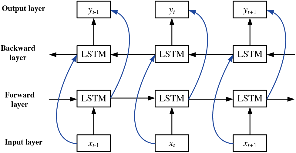
Figure 1: Schematic diagram of the structure of a BLSTM neural network

ft=σ(Wxfxt+Whfht−1+bf)(1a)

it=σ(Wxixt+Whiht−1+bi)(1b)

ot=σ(Wxoxt+Whoht−1+bo)(1c)

where xt denotes the input vector at time step t, ht−1 is the output vector at time step t−1, σ(.) is the sigmoid activation function, Wxf, Whf, Wxi, Whi, Wxo and Who are the weight matrices, and bf, bi and bo are the bias vectors.

The cell states vector ct at time step t is obtained as with [45]

ct=ft∘ct−1+it∘tanh(Wxcxt+Whcht−1+bc)(2)

where ∘ denotes the Hadamard product.

The output vector ht of memory cells at time step t is given by

ht=ot∘tanh(ct)(3)

To take into account future information, the BLSTM includes forward and backward LSTM layers, and the inputs from the LSTM layers are treated simultaneously by the output layer. The neural network is updated as follows [45]:

ht=H(W1xt+W2ht−1+b)(4a)

h¯t=H(W3xt+W5h¯t−1+b¯)(4b)

yt=H(W4xt+W6ht−1+by)(4c)

where ht and h¯t are the vectors for backward and forward propagation layer, respectively, yt is the vector for an output layer, and b, b¯ and by are the bias vectors. W1∼W6 are the weight coefficients.

Bayesian optimization may be employed to obtain good results after a few iterations and we follow this strategy to obtain the hyperparameters of our BLSTM network [49]. To assess the performance of the model, we employ the root mean square error (RMSE) as well as the mean absolute error (MAE) and the determination coefficient (R2) are used. They are defined as follows:

RMSE=∑j=1n(yi−yi^)2n(5a)

MAE=∑j=1n∣yi−yi^∣n(5b)

R2=1−∑j=1n(yi−yi^)2∑j=1n(yi−y¯)2(5c)

where n denotes the number of samples, yi, yi^ are the actual and forecasted values of the ith sample of the prediction group, respectively, and y¯ is the average value of the prediction group.

Concerning the sequence-to-sequence regression network, the loss function of the regression layer is another evaluation index, i.e.,

LOSS=12S∑i=1S∑j=1R(tij−yij)2(6)

In the above equation, S is the sequence length, R is the number of prediction values, tij is the target output, and yij is the prediction value.

A data set containing inputs and outputs for large samples is required for developing a deep learning solution. Those data are used to train the BLSTM model and optimize performance. In turn, the prediction accuracy is directly affected by the quality and quantity of the data and the quality of the data set is a relevant ingredient to develop an effective network. The S-FSDT-based IGA combined with von Kármán theory is here employed to obtain the target variable for each sample.

3  IGA Simulations with S-FSDT

In this work, the material parameters of FG plate are assumed to vary along the thickness with a power law distribution.

P(z)=Pm+(Pc−Pm)(12+zt)k(7)

where t is the plate thickness, P represents Young’s modulus E, and the Poisson’s ratio is ν. The gradient index is k, whereas z denotes the thickness variable with range −t/2≤z≤t/2. The subscripts c and m stand for “ceramic” and “metal”, respectively.

In the S-FSDT approach, the displacement field is given by [7]

u(x,y,z)=u0(x,y)−zwb,x(x,y)(8a)

v(x,y,z)=v0(x,y)−zwb,y(x,y)(8b)

w(x,y,z)=wb(x,y)+ws(x,y)(8c)

where u0 and v0 are the displacements in the x and y directions on the plate mid-plane, respectively, and wb and ws denote the bending and shear components of the transverse displacement, respectively.

Compared to the traditional FSDT, S-FSDT requires one less variable but it requires C1 continuity of the bending component wb.

The strain-displacement nonlinear relations are given by [7]

ε={εm00}+{−zεb0εs0}+{−zεmnl0}(9)

with

ε=[εxεyγxyγxzγyz]T,εm0={u0,xv0,yu0,y+v0,x},εb0={wb,xxwb,yy2wb,xy}(10a)

εs0={ws,xws,y},εmnl=12[wb,x+ws,x00wb,y+ws,ywb,y+ws,ywb,x+ws,x]{wb,x+ws,xwb,y+ws,y}(10b)

According to standard elastic theory, the stresses are written as

σ=Dε(11)

with

σ=[σxσyτxyτxzτyz]T(12a)

D=[Dm00Ds],Dm=E1−ν2[1ν0ν10001−ν2],Ds=αE2(1+ν)[1001](12b)

where α denotes the shear correction factor, set to k=5/6 in our paper.

The displacements on the middle plane of plate are expressed in the NURBS basis functions as

u0h(ξ)=∑i=1NPRi(ξ)ui(13)

with

u0h=[u0hv0hwbhwsh]T(14a)

ui=[uiviwbiwsi]T(14b)

where NP denotes the number of all the control points in the computation mesh, ξ is the parametric coordinate, ui and Ri(ξ) denote the unknown displacement vector and the NURBS basis function at control point i, respectively.

Using Eqs. (13) and (9), we obtain the relation between the incremental strain vector and the incremental displacement vector. We have

dε=B¯due(15)

with

B¯={Bm0}+{zBbBs}+{ABnl0}(16)

Bm=[Bm1⋯Bmi⋯BmNP],Bmi=[Ri,x0000Ri,y00Ri,yRi,x00](17a)

Bb=[Bb1⋯Bbi⋯BbNP],Bbi=[00Ri,xx000Ri,yy0002Ri,xy0](17b)

Bs=[Bs1⋯Bsi⋯BsNP],Bsi=[000Ri,x000Ri,y](17c)

Bnl=[Bnl1⋯Bnli⋯BnlNP],Bnli=[00Ri,xRi,x00Ri,yRi,y](17d)

A=[wb,x+ws,x00wb,y+ws,ywb,y+ws,ywb,x+ws,x](17e)

where due=[du1du2...duNP]T denotes the incremental displacement vector at control points.

The governing equations can be obtained using the virtual work principle. They are nonlinear and can be solved with the Newton-Raphson iterative method [7].

4  Data Set Preparation Using IGA Simulations

In deep learning, a data set that includes the desired inputs and outputs is required, and the quality and quantity of the data determine the achievable accuracy.

The procedures of data set preparation used in this study are the following: For the first example, different values of the uniform load q are considered, i.e., q=q0×(1,2,…,50) units. The gradient index k ranges from 0.1 to 0.4, and the deflection value of the plate center is predicted for k = 0.5. For the last two examples, different values of the uniform load q are considered, i.e., q=q0×(1,2,…,60) units. The gradient index k ranges from 0.4 to 4, and ten gradient indices are considered by evenly dividing the gradient index range, i.e., k=0.4,0.8,…,4. For a given gradient index value, the uniform load takes a value from q=q0×(1,2,…,60) units. Therefore, 600 data obtained by IGA are used as datasets. We then split data into training and test sets for the BLSTM model learning. The first 500 values for k=0.4,0.8,…,4 and q=q0×(1,2,…,50) units are used as the training set, the remaining 100 data for k=0.4,0.8,…,4 and q=q0×(51,52,…,60) units are used as the test set.

In the training stage, we use the value of q=q0×(1,2,…,50) units when k=0.4,0.8,…,3.6 to predict the value of q=q0×(1,2,…,50) units when k=4. Correspondingly, in the test stage, we use the value of q=q0×(51,52,…,60) units when k=0.4,0.8,…,3.6 to predict the value of q=q0×(51,52,…,60) units when k=4. Finally, we compare the ten deflection values predicted when k=4 and q=q0×(51,52,…,60) units in the test set with the target values to verify the effectiveness of the deep learning model.

5  Numerical Examples

We now present the results obtained for three paradigmatic examples to show the reliability of our model. Four hyperparameters (i.e., the number of dropout layers N1, the number of cells N2, the learning rate, and the L2 regularization) are determined by Bayesian optimization. Their ranges are given in Table 1.

The number of dropout layers is used to avoid overfitting, the initial learning rate is used for training. If the learning rate is too low, it may lead to a training time too long. If the learning rate is too high, then the training may achieve a suboptimal result. L2 regularization (L2 norm) is used to avoid overfitting. Finally, the other parameters of the BLSTM algorithm are set as follows: max epochs are set to 50, minibatch size to 16, dropout value to 0.2, maxitration number to 20, learn rate drop period to 25, and learn rate drop factor to 0.4.

5.1 A Square Titanium Alloy/Aluminum Oxide Plate

In our first example, we consider a square plate made of Ti-6Al-4V/aluminum oxide with length a= 10 units and thickness t = 0.5 units subject to a uniform load q. The plate parameters are set as follows: Ec=320.2×109 units, νc=0.26, Em=105.7×109 units, and νm=0.298. The deflection of the center (CD) is normalized by w¯=w/t, and q0=1.15×106.

After Bayesian optimization, we obtain N1=1 and N2=77. The learning rate is 0.05, and the L2 regularization is set to 6.69×10−7. From Fig. 2, we see that RMSE and LOSS decrease during the training process. The regression evaluation indexes, which are used to evaluate the prediction accuracy of the model, are RMSE = 0.016, MAE = 0.010 and R2 = 0.99.

Figure 2: Dynamics of the training: light curves and dark curves are training and smoothed training curves, respectively

The targets and outputs of the CD for different normalized loads P=q0a4/(Emt4) at the central point are shown in Fig. 3. From Fig. 3, we see that the normalized CD of the FG plate calculated by BLSTM agree with those obtained by S-FSDT-based IGA [7] and by two FSDT-based methods: the element-free kp-Ritz [4] and the local Petrov-Galerkin with moving Kriging interpolation (PGMK) ones [5], which confirms the accuracy of our method.

Figure 3: Load-deflection curve at the central point

5.2 A Square Aluminum/Alumina Plate

In the second example, we consider an aluminum/alumina (Al/Al2O3) square FG plate of length L = 10 units and thickness t= 1 unit subject to a uniform pressure q. The plate parameters are set as follows: Ec=380×109 units, νc=0.3, Em=70×109 units, and νm=0.3. The CD is normalized as w¯=w/t, and q0=2×108.

After Bayesian optimization, we obtain N1=1 and N2=86. The learning rate is 0.01, and the L2 regularization is set to 2.86×10−10. The regression evaluation indexes are employed to assess the prediction accuracy of the model. As it is apparent from Fig. 4, the RMSE and LOSS gradually decrease during the training progress. In the training, the values of regression evaluation indexes are: RMSE = 0.016, MAE = 0.014 and R2 = 0.96.

Figure 4: The training dynamics: light and dark curves are training curves and smoothed training curves, respectively

The targets and the outputs of the CD for different normalized loads P=qL4/(Ect4) at the central point are shown in Fig. 5. The outputs are obtained by the machine learning model. From Fig. 5, we see that the load-deflection curve is nonlinear, this indicates that nonlinear bending of FG plate occurs. In other words, the present model can directly estimate the displacement of the FG plate for large deformations. Table 2 illustrates the results for the predicted CD. They match well the actual values, demonstrating the high accuracy of our machine learning model.

Figure 5: Load-deflection curve at the central point

5.3 A Circular Aluminum/Zirconia Plate

The third example is that of a clamped circular FG plate made of aluminum and zirconia (Al/ZrO2) with radius r = 1 unit and thickness t= 0.1 units under a uniform load q. The plate parameters are set as follows: Ec=151×109 units, νc=0.3, Em=70×109 units, νm=0.3. The CD is normalized by w¯=w/t, and q0=106.

After Bayesian optimization, N1=4, N2=85, the learning rate is 0.01, and the L2 regularization is 1.06×10−10. For the training process of BLSTM, the variations of RMSE and loss function are respectively plotted in Fig. 6. In this training, the values of regression evaluation indexes are as follows: RMSE = 0.014, MAE = 0.013 and R2 = 0.99.

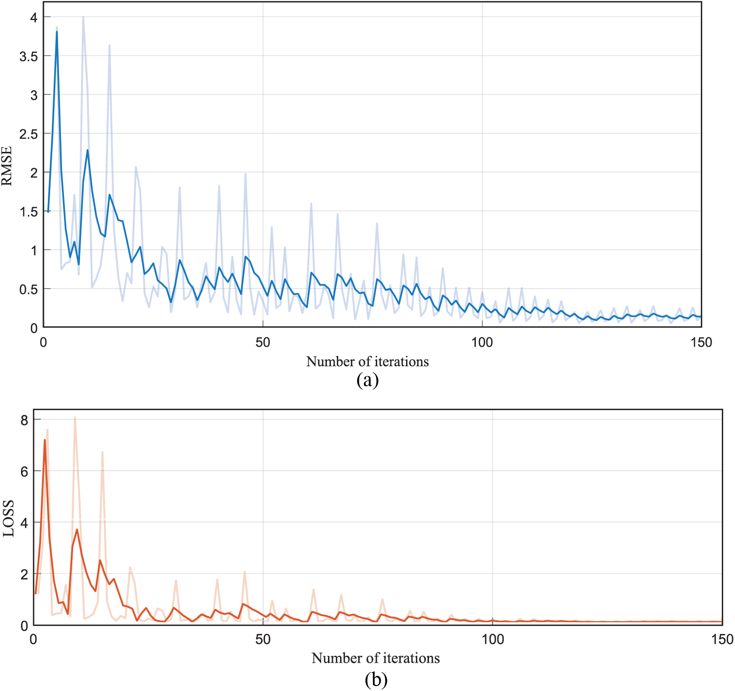
Figure 6: Dynamics of the training: light and dark curves are training curves and smoothed training curves, respectively

In Fig. 6, one can see that after 150 iterations, the RMSE and loss function of the model are already very low, i.e., the BLSTM model has been properly trained and no over-fitting can be observed. The trained BLSTM model can be then used to make predictions for the testing datasets. Fig. 7 shows the targets and outputs of the CD for different normalized loads P=qr4/(Emt4) at the central point. The outputs are obtained by the machine learning model and the nonlinear character of the load-deflection curve is apparent, i.e., our model can directly estimate the nonlinear bending of the FG plate.

Figure 7: Load-deflection curve at the central point

The predicted normalized CD for different normalized load parameters using the machine learning model is reported in Table 3. The relative error is rather small. The average error is 0.013, and the standard deviation of the error is 0.003, proving the high accuracy of our deep learning model.

6  Conclusions and Outlook

In this paper, we have presented and analyzed a deep learning method for forecasting the geometrically nonlinear bending behavior of FG plates, thus bypassing the complex simulation processes usually involved in this kind of investigation. In our BLSTM recurrent neural network, the load and gradient indexes are assigned as the inputs, whereas the displacement responses are set as outputs. The hyperparameters of the model, which influence the training process and determine the accuracy of the model, are determined by Bayesian optimization.

The nonlinear relationship between the outputs and the inputs is obtained by machine learning, such that the displacements can be directly estimated by the deep learning network. The S-FSDT-based IGA combined with von Kármán theory is used to obtain the training data, i.e., the displacement responses for different loads and gradient indexes. Numerical results indicate that the recognition error is low, and it demonstrates the feasibility of using the deep learning technique as a fast and accurate alternative to IGA for modeling the geometrically nonlinear bending of FG plates.

The limitations of the FSDT and S-FSDT concern inaccuracy in the distribution of transverse shear stress and the fact that the traction-free boundary conditions at the two surfaces are violated. Hence, the shear correction factor, which is difficult to choose appropriately, is needed to modify the distribution of the transverse shear stress. The refined plate theories [50] can be exploited instead of a shear correction factor, leading to more accurate and robust results. In this approach, the generalized displacements should be C1-continuous and this requirement can be readily satisfied within IGA. In the future, we plan to integrate the refined plate theories into our codes and extend the present method to FG shells [51].

Acknowledgement: The authors thank the referees for their suggestions, which contributed to improve the presentation of our results.

Funding Statement: TTY acknowledges the support from the National Natural Science Foundation of China (NSFC) under Grant Nos. 12272124 and 11972146.

Author Contributions: The authors’ contribution are the following: study conception and design: SL, TTY; data collection: SL; analysis and interpretation of results: SL, TTY, TQB; draft manuscript preparation: SL, TTY, TQB. All authors reviewed the results and approved the final version of the manuscript.

Availability of Data and Materials: Data will be made available upon reasonable request.

Conflicts of Interest: The authors declare that they have no conflicts of interest to report regarding the present study.

References

1. Gunes, R., Reddy, J. N. (2008). Nonlinear analysis of functionally graded circular plates under different loads and boundary conditions. International Journal of Structural Stability and Dynamics, 8(1), 131–159. [Google Scholar]

2. Na, K. S., Kim, J. H. (2006). Thermal postbuckling investigations of functionally graded plates using 3-D finite element method. Finite Elements in Analysis and Design, 42(8/9), 749–756. [Google Scholar]

3. Praveen, G. N., Reddy, J. N. (1998). Nonlinear transient thermoelastic analysis of functionally graded ceramic-metal plates. International Journal of Solids and Structures, 35(33), 4457–4476. [Google Scholar]

4. Zhao, X., Liew, K. M. (2009). Geometrically nonlinear analysis of functionally graded plates using the element-free kp-Ritz method. Computer Methods in Applied Mechanics and Engineering, 198(33–36), 2796–2811. [Google Scholar]

5. Zhu, P., Zhang, L. W., Liew, K. M. (2014). Geometrically nonlinear thermomechanical analysis of moderately thick functionally graded plates using a local Petrov-Galerkin approach with moving Kriging interpolation. Composite Structures, 107, 298–314. [Google Scholar]

6. Zhang, L. W., Lei, Z. X., Liew, K. M., Yu, J. L. (2014). Large deflection geometrically nonlinear analysis of carbon nanotube-reinforced functionally graded cylindrical panels. Computer Methods in Applied Mechanics and Engineering, 273, 1–18. [Google Scholar]

7. Yu, T. T., Yin, S. H., Bui, T. Q., Hirose, S. (2015). A simple FSDT-based isogeometric analysis for geometrically nonlinear analysis of functionally graded plates. Finite Elements in Analysis and Design, 96(18–19), 1–10. [Google Scholar]

8. Yin, S. H., Yu, T. T., Bui, T. Q., Nguyen, M. N. (2015). Geometrically nonlinear analysis of functionally graded plates using isogeometric analysis. Engineering Computations, 32(2), 519–558. [Google Scholar]

9. Deng, L., Yu, D. (2014). Deep learning: Methods and applications. Foundations and Trends® in Signal Processing, 7(3–4), 197–387. [Google Scholar]

10. Schmidhuber, J. (2015). Deep learning in neural networks: An overview. Neural Networks, 61(3), 85–117. [Google Scholar] [PubMed]

11. Jung, S., Ghaboussi, J. (2006). Characterizing rate-dependent material behaviors in self-learning simulation. Computer Methods in Applied Mechanics and Engineering, 196(1–3), 608–619. [Google Scholar]

12. Reuter, U., Sultan, A., Reischl, D. S. (2018). A comparative study of machine learning approaches for modeling concrete failure surfaces. Advances in Engineering Software, 116(2), 67–79. [Google Scholar]

13. Raissi, M., Karniadakis, G. E. (2018). Hidden physics models: Machine learning of nonlinear partial differential equations. Journal of Computational Physics, 357(4), 125–141. [Google Scholar]

14. Nguyen, T. N., Nguyen-Xuan, H., Lee, J. (2020). A novel data-driven nonlinear solver for solid mechanics using time series forecasting. Finite Elements in Analysis and Design, 171(3), 103377. [Google Scholar]

15. Haghighat, E., Raissi, M., Moure, A., Gomez, H., Juanes, R. (2021). A physics-informed deep learning framework for inversion and surrogate modeling in solid mechanics. Computer Methods in Applied Mechanics and Engineering, 379(7553), 113741. [Google Scholar]

16. Nguyen, L. T. K., Keip, M. A. (2018). A data-driven approach to nonlinear elasticity. Computers and Structures, 194, 97–115. [Google Scholar]

17. Kim, C., Lee, J., Yoo, J. (2021). Machine learning-combined topology optimization for functionary graded composite structure design. Computer Methods in Applied Mechanics and Engineering, 387, 114158. [Google Scholar]

18. Abueidda, D. W., Koric, S., Sobh, N. A. (2020). Topology optimization of 2D structures with nonlinearities using deep learning. Computers and Structures, 237, 106283. [Google Scholar]

19. Chi, H., Zhang, Y., Tang, T. L. E., Mirabella, L., Dalloro, L. et al. (2021). Universal machine learning for topology optimization. Computer Methods in Applied Mechanics and Engineering, 375(2), 112739. [Google Scholar]

20. Feng, Y., Wang, Q. H., Wu, D., Luo, Z., Chen, X. J. et al. (2021). Machine learning aided phase field method for fracture mechanics. International Journal of Engineering Science, 169(14), 103587. [Google Scholar]

21. Carrara, P., Ortiz, M., de Lorenzis, L. (2021). Data-driven rate-dependent fracture mechanics. Journal of the Mechanics and Physics of Solids, 155, 104559. [Google Scholar]

22. Liu, X., Athanasiou, C. E., Padture, N. P., Sheldon, B. W., Gao, H. J. (2020). A machine learning approach to fracture mechanics problems. Acta Materialia, 190(15), 105–112. [Google Scholar]

23. Yang, C., Yang, X., Xiao, X. (2016). Data-driven projection method in fluid simulation. Computer Animation and Virtual Worlds, 27(3–4), 415–424. [Google Scholar]

24. Han, Z. Q., De, S. (2019). A deep learning-based hybrid approach for the solution of multiphysics problems in electrosurgery. Computer Methods in Applied Mechanics and Engineering, 357(9), 112603. [Google Scholar] [PubMed]

25. Jung, J., Yoon, K., Lee, P. S. (2020). Deep learned finite elements. Computer Methods in Applied Mechanics and Engineering, 372, 113401. [Google Scholar]

26. Jung, J., Jun, H., Lee, P. S. (2022). Self-updated four-node finite element using deep learning. Computational Mechanics, 69(1), 23–44. [Google Scholar]

27. Korzeniowski, T. F., Weinberg, K. (2021). A multi-level method for data-driven finite element computations. Computer Methods in Applied Mechanics and Engineering, 379(11), 113740. [Google Scholar]

28. Lin, S., Zheng, H., Han, C., Han, B., Li, W. (2021). Evaluation and prediction of slope stability using machine learning approaches. Frontiers of Structural and Civil Engineering, 15(4), 821–833. [Google Scholar]

29. Husken, M., Stagge, P. (2003). Recurrent neural networks for time series classification. Neurocomputing, 50(2), 223–235. [Google Scholar]

30. Hochreiter, S., Schmidhuber, J. (1997). Long short-term memory. Neural Computation, 9(8), 1735–1780. [Google Scholar] [PubMed]

31. Wang, Z., Xiao, D., Fang, F., Govindan, R., Pain, C. C. et al. (2018). Model identification of reduced order fluid dynamics systems using deep learning. International Journal for Numerical Methods in Fluids, 86(4), 255–268. [Google Scholar]

32. Qu, X., Yang, J., Chang, M. (2019). A deep learning model for concrete dam deformation prediction based on RS-LSTM. Journal of Sensors, 2019(1), 4581672. [Google Scholar]

33. Yang, S. L., Han, X. J., Kuang, C. F., Fang, W. H., Zhang, J. F. et al. (2022). Comparative study on deformation prediction models of Wuqiangxi concrete gravity dam based on monitoring data. Computer Modeling in Engineering and Sciences, 131(1), 49–72. [Google Scholar]

34. Liu, W., Pan, J., Ren, Y., Wu, Z., Wang, J. (2020). Coupling prediction model for long-term displacements of arch dams based on long short-term memory network. Structural Control and Health Monitoring, 27(7), e2548. [Google Scholar]

35. Law, R., Li, G., Fong, D. K. C., Han, X. (2019). Tourism demand forecasting: A deep learning approach. Annals of Tourism Research, 75(1), 410–423. [Google Scholar]

36. Nguyen-Le, D. H., Tao, Q. B., Nguyen, V. H., Abdel-Wahab, M., Nguyen-Xuan, H. (2020). A data-driven approach based on long short-term memory and hidden Markov model for crack propagation prediction. Engineering Fracture Mechanics, 235(2), 107085. [Google Scholar]

37. Fan, D., Sun, H., Yao, J., Zhang, K., Yan, X. et al. (2021). Well production forecasting based on ARIMA-LSTM model considering manual operations. Energy, 220(6), 119708. [Google Scholar]

38. Zhang, N., Shen, S., Zhou, A., Jin, Y. (2021). Application of LSTM approach for modelling stress-strain behaviour of soil. Applied Soft Computing Journal, 100(10), 106959. [Google Scholar]

39. Arsenault, R., Martel, J. L., Brunet, F., Brissette, F., Mai, J. L. E. (2023). Continuous streamflow prediction in ungauged basins: Long short-term memory neural networks clearly outperform traditional hydrological models. Hydrology and Earth System Sciences, 27(1), 139–157. [Google Scholar]

40. Shahid, F., Zameer, A., Muneeb, M. (2020). Predictions for COVID-19 with deep learning models of LSTM, GRU and Bi-LSTM. Chaos, Solitons and Fractals, 140(14), 110212. [Google Scholar] [PubMed]

41. Xia, T., Song, Y., Zheng, Y., Pan, E., Xi, L. (2020). An ensemble framework based on convolutional bi-directional LSTM with multiple time windows for remaining useful life estimation. Computers in Industry, 115, 103182. [Google Scholar]

42. Yildirim, O. (2018). A novel wavelet sequence based on deep bidirectional LSTM network model for ECG signal classification. Computers in Biology and Medicine, 96, 189–202. [Google Scholar] [PubMed]

43. Subbiah, S. S., Paramasivan, S. K., Arockiasamy, K., Senthivel, S., Thangavel, M. (2023). Deep learning for wind speed forecasting using Bi-LSTM with selected features. Intelligent Automation and Soft Computing, 35(3), 3829–3844. https://doi.org/10.32604/iasc.2023.030480 [Google Scholar] [CrossRef]

44. Wollmer, M., Eyben, F., Graves, A., Schuller, B., Rigoll, G. (2010). Bidirectional LSTM networks for context-sensitive keyword detection in a cognitive virtual agent framework. Cognitive Computation, 2(3), 180–190. [Google Scholar]

45. Kulshresth, A., Krishnaswamy, V., Sharma, M. (2020). Bayesian BILSTM approach for tourism demand forecasting. Annals of Tourism Research, 83(2), 102925. [Google Scholar]

46. Hughes, T. J. R., Cottrell, J. A., Bazilevs, Y. (2005). Isogeometric analysis: CAD, finite elements, NURBS, exact geometry and mesh refinement. Computer Methods in Applied Mechanics and Engineering, 194(39–41), 4135–4195. [Google Scholar]

47. Zhang, Q., Nguyen-Thanh, N., Li, W. D., Zhang, A. M., Li, S. F. et al. (2023). A coupling approach of the isogeometric-meshfree method and peridynamics for static and dynamic crack propagation. Computer Methods in Applied Mechanics and Engineering, 410(39–41), 115904. [Google Scholar]

48. Thai, H. T., Choi, D. H. (2013). A simple first-order shear deformation theory for the bending and free vibration analysis of functionally graded plates. Composite Structures, 101(1–3), 332–340. [Google Scholar]

49. Law, T., Shawe-Taylor, J. (2017). Practical Bayesian support vector regression for financial time series prediction and market condition change detection. Quantitative Finance, 17(9), 1403–1416. [Google Scholar]

50. Senthilnathan, N. R., Lim, S. P., Lee, K. H., Chow, S. T. (1987). Buckling of shear-deformable plates. AIAA Journal, 25(9), 1268–1271. [Google Scholar]

51. Ramezani, M., Rezaiee-Pajand, M., Tornabene, F. (2022). Nonlinear dynamic analysis of FG/SMA/FG sandwich cylindrical shells using HSDT and semi ANS functions. Thin-Walled Structures, 171(8), 108702. [Google Scholar]