Analytical and Numerical Methods to Study the MFPT and SR of a Stochastic Tumor-Immune Model

1  Introduction

In recent years, a varieties of tumor diseases have been observed and brought a revolution in the field of cancer treatment. In order to explore the law of tumor growth and extinction, a good many of researchers dedicate to study the tumor models, the issues including the growth of anti-tumor, the competition between the tumor cells and the immune system [1–5].

Some deterministic tumor models such as Logistic model [6], Gompertz model [7] have been proved to be the powerful models to describe the dynamical evolution of the tumor, these models are not only helpful for understanding the competition between the tumor cells and the immune system, but also beneficial for assisting the tumor’s elimination or extinction. However, in recent decades, scholars began to realize that these deterministic models are not consistent with the reality enough because they ignore the effects of environmental perturbations. In fact, the growth of the malignant tumors relies heavily on the synthesis of the proteins which are very sensitive to the environmental perturbations [8–10]. However, uncertain factors such as body temperature, blood pressure, oxygen level, and others in cells’ microenvironment can bring the random fluctuation to the population of the tumor cells and the immune cells. Therefore, stochastic dynamical models regarding to the tumor and the immune system are gradually proposed instead of the deterministic ones [11–13], in which the mentioned uncertain microenvironment is usually modeled by random noises with a certain probability distribution.

Some valuable works have been achieved for the stochastic tumor or tumor-immune models. In 2012, Li et al. [14] considered a tumor growth model perturbed by a Gaussian white noise together with a dichotomous noise, he used the Mean First Extinction Time (MFET) as an index to analyze the transitions from the steady state to the extinction state of the tumor cells. In 2018, Ochab-Marcinek et al. [15] studied how dichotomous noise and Gaussian white-noise affected the MFET of the cell population in a tumor-immune model. They observed the important dynamical phenomena of Resonance Activation (RA) and Noise Enhanced Stability (NES). In 2020, Han et al. [16] discussed the tumor growth model under the immune surveillance with stochastic fluctuations modelled as Gaussian white noises, he defined the extinction time as the time when the tumor firstly escaped to the extinction state from the steady state, and simulated the effect of different noise parameters on the most probable extinction time. In 2022, the first author of this paper [17] discussed MFET from the steady-state state to the extinction state in a stochastic tumor-immune model with Gaussian white-noises, they discovered the phenomena of the NES as well as Stochastic Resonant (SR).

Based on the current references above, we summarize that the stochastic tumor models especially stochastic tumor-immune models regarding tumor state transition are concentrated on the Gaussian white-noise or dichotomous noise perturbation. However, the significant noise perturbations such as color noise or non-Gaussian noises are seldom mentioned in the existing literature. According to the authors’ knowledge, only [18] considered a tumor growth model perturbed by Gaussian colored noise in 2022, and this paper studied the noise-induced phenomenon of the transition from a steady state to an extinction state by MFET.

In addition, we have to mention that the previous works mainly focus on the issue of the MFPT from the steady state to the extinction state. The reason for this is that people care much about the time for a human body from a tumor-present state to a healthy state. That is, the time probably for a person to be cured well from the tumor state is an important purpose of the tumor treatment. Nevertheless, it is true that tumor recurrence is a typical feature of tumors compared with others disease especially the malignant tumors; how long will it take to be recurrent for a tumor patient after a previous recovery? It is also extremely important issue concerned in the tumor treatment. Therefore, the discussion for MFPT from the extinction state to the steady state in a tumor-immune model is also definitely necessary and significant, this is exactly one of the key innovation of this paper.

Since the MFPT is a significant index used to describe the noise-induced escape process in stochastic tumor-immune models, how to obtain this index and how to solve the governing equations become the following task. Generally, MFPT is governed by a back-forward partial differential equation with nonlinear functional coefficients, the developing methods such as finite difference method [19,20], path integral method [21] and Galerkin method [22,23] are common used to solve a partial differential equation. However, these methods usually have strict requirements for the dimension or domain mesh, the accuracy and computer running time can not be balanced at the same time. Back-Propagation Neural Network (BPNN) has been proved to be a viable, multipurpose and robust computational methodology with solid theoretic support and strong potential applications [24,25]. Many existing studies have shown the approximation ability of BPNN to nonlinear functions as well as the efficiency in solving solution of the nonlinear models [26]. It is interesting to see that BPNN is not much applied to study MFPT problem in the field of the stochastic dynamical system, which inspires us to extend this algorithm to the case of the tumor-immune model.

On the other hand, Stochastic Resonance (SR) is a dynamical phenomenon usually happened in a stochastic dynamical system, refer to the response to an input signal enhanced by the optimal amount of noise. Owing to the role of the SR, it has been mentioned in certain tumor-immune research as one of the indexes to measure the tumor dynamics. The representative works with regard to the SR include that Li et al. [27] derived a theory for the SR by using the two-state approach in 2011, and obtained the corresponding signal-to-noise ratio (SNR). It is found that in subthreshold periodic treatment, weak environmental fluctuations can induce the extinction of the tumor cells. In 2018, Shi et al. [28] considered the SR of asymmetric bistable systems with multiplicative white noise and additive color noise, and studied the influence of parameters on the SR from the perspective of the SNR. In 2021, Guo et al. [29] established the tumor growth model excited by a Levy noise and a Gaussian white noise, he studied the relationship between the SNR and the noise intensity by a kind of numerical simulation, and obtained a conclusion that all parameters in the model can induce the SR. It can be seen that the SNR is the most commonly used index in SR research. Therefore, this paper also uses SNR to describe and analyze the phenomenon of the SR.

To sum up, this paper aims to improve the current research about the stochastic tumor-immune model from four points: (1) Considering color noise to be the random perturbation in the cell microenvironment; (2) Focusing on the transition from the tumor extinction to the tumor recurrence; (3) Using two methods of the analytical process and numerical algorithm to obtain the indexes of the MFPT and the SR; (4) Applying the BPNN to solve the governing the MFPT and the SR equations to testify the correction and effectiveness of the proposed methods.

2  Stochastic Tumor-Immune Model with Correlated Noises

The interaction between the tumor cells and the immune system can be illustrated by Fig. 1 based on Michaelis-Menten enzymatic reaction. Correspondingly, the mathematical model governing the tumor growth under the immune surveillance can be expressed by a differential equation after a series of mathematical procedure [17] as

dxdt=x(1−θx)−βx1+x,(1)

where x(t) is a function of the time t, represents the normalized population of the tumor cells, the parameter θ is the environmental capacity, and the coefficient β expresses the relative rate of the tumor extinction. Correspondingly, the potential function of Eq. (1) is

U(x)=−x22+θx33+βx−βln⁡(x+1),(2)

where U(x) has two steady-state solutions, which are the extinction state x1 and the tumor-present state x2, respectively:

x1=0,(3)

x2=1−θ+(1+θ)2−4βθ2θ,(4)

and one unstable state solution

xu=1−θ−(1+θ)2−4βθ2θ.(5)

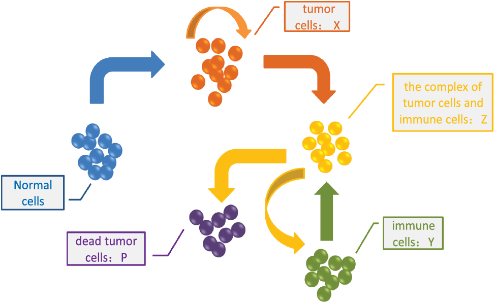
Figure 1: The interaction between tumor cells and immune system

Considering that most biochemical systems in reality are open systems, they often exchange the information and the energy through the interaction with the outside world. So it is necessary to consider the impact of the environmental fluctuations on the systems, which are often modeled as noise in the mathematical models. In this section, we will model the environmental fluctuations in the tumor-immune model Eq. (1) as multiplicative Gaussian colored noise ξ(t) and additive Gaussian white noise η(t) to construct a stochastic tumor-immune model

dxdt=x(1−θx)−βxx+1−xx+1ξ(t)+η(t),(6)

where the noises ξ(t) and η(t) have the following statistical properties:

⟨ξ(t)⟩=0,⟨ξ(t)ξ(s)⟩=D1τexp[−1τδ(t−s)],⟨η(t)⟩=0,⟨η(t)η(s)⟩=2D2δ(t−s),(7)

in which D1 and D2 are the intensities of multiplicative noise ξ(t) and additive noise η(t), respectively, τ is the auto-correlation time, and ⟨⟩ is the operator of the mathematical expectation. Especially, the multiplicative Gaussian colored noise ξ(t) can be derived from a linear filter on the basis of another Gaussian white noise ε(t), which is correlated with noise η(t), that is

dξdt=−1τξ+1τε(t),(8)

and

⟨ε(t)⟩=0,⟨ε(t)ε(s)⟩=2D1δ(t−s),⟨ε(t)η(s)⟩=⟨η(t)ε(s)⟩=2λD1D2δ(t−s),(9)

where λ is the cross-correlation intensity between ε(t) and η(t).

3  Stochastic Dynamics for SPD, MFPT, and SR

3.1 Theoretic Solution for SPD

Due to the existence of the colored noises, we know that Eq. (6) is a one-dimensional non-Markovian process, which means that the Fokker-Planck equation describing the probability density of the tumor cells cannot be obtained directly. Therefore, we will deal with this problem through the theory of Unified Colored Noise Approximation (UCNA) to obtain an approximate Markovian process and AFPE [30]. For convenience, we rewrite Eq. (6) as

dxdt=h(x)+g1(x)ξ(t)+g2(x)η(t).(10)

Correspondingly,

h(x)=x(1−θx)−βxx+1,g1(x)=−xx+1,g2(x)=1.(11)

Firstly, through some transformations associated with the UCNA method, we can obtain the following one-dimensional approximate Markovian process from Eqs. (6)–(9), that is

dxdt=h(x)C(x,τ)+1C(x,τ)[g1(x)ε(t)+g2(x)η(t)]=h∗(x)+g∗(x)ζ(t),(12)

where ζ(t) is also a Gaussian white noise with zero mean and

⟨ζ(t)ζ(s)⟩=2δ(t−s).(13)

Instead, the expressions of h∗(x) and g∗(x) can be denoted by way of an auxiliary function C(x,τ), i.e.,

C(x,τ)=1−τ[h′(x)−g1′(x)g1(x)h(x)],h∗(x)=h(x)C(x,τ),g(x)=[D1g12(x)+2λD1D2g1(x)g2(x)+D2g22(x)]12,g∗(x)=g(x)C(x,τ).(14)

Finally, the AFPE corresponding to Eq. (6) can be described as

∂P1(x,t)∂t=−∂∂x[A1(x)P1(x,t)]+∂2∂x2[B1(x)P1(x,t)],(15)

where P1(x,t) is the transient probability density of the tumor cells at the time t, A1(x) and B1(x) are called the drift function and the diffusion function, respectively, and

A1(x)=h∗(x)+g∗(x)g∗′(x),B1(x)=g∗2(x),(16)

so the expressions corresponding to A1(x) and B1(x) can be written as

A1(x)=x(1−θx)−βxx+11−τ(1−2θx−1−θxx+1)+D1x(x+1)3−λD1D21(x+1)2[1−τ(1−2θx−1−θxx+1)]2+τ[−2θ+1+θ(x+1)2][1−τ(1−2θx−1−θxx+1)]3[D1x2(x+1)2−2λD1D2xx+1+D2],(17)

B1(x)=1[1−τ(1−2θx−1−θxx+1)]2[D1x2(x+1)2−2λD1D2xx+1+D2].(18)

Basically, the evolution of the tumor cells under the immune surveillance is a long-term process, so we generally concerns the stationary probability density of the tumor cells, which means the case of t→∞ in Eq. (15). Therefore, The AFPE describing the SPD Ps1(x) can be rewritten as

−∂∂xA1(x)Ps1(x)+∂2∂x2B1(x)Ps1(x)=0,(19)

its boundary condition and normalization condition are, respectively

Ps1(x)=0ifx∈∂Ω0,(20)

and

∫0+∞Ps1(x)dx=1,(21)

where ∂Ω0 is the boundary of the definition domain Ω0 of the tumor cells. Then the SPD can be obtained by solving the following integral:

Ps1(x)=N11B1(x)exp[∫xA1(u)B1(u)du]=N11B1(x)exp[−V1(x)D1],(22)

where N1 is the normalization coefficient; V1(x) is the generalized potential function, which is governed by

V1(x)=−∫x[x(1−θx)−βxx+1]1−τ(1−2θx−1−θxx+1)x2(x+1)2−2λD2D1xx+1+D2D1dx=1g0[g1x4+g2x3+g3x2+g4x+c12ln|x2+b1x+b2|+2c2−c1b1−b12+4b2arctan2x+b1−b12+4b2],(23)

in which

g1=14a1,g2=13(a2−a1b1),g3=12(a3−a1b2−a2b1+a1b12),g4=a4−a2b2+2a1b1b2−a3b1+a2b12−a1b13,c1=a5−a3b2+a1b22+a2b1b2−a1b12b2−b1(a4−a2b2+a1b1b2−a3b1+a1b1b2+a2b12−a1b13),c2=b2(a4−a2b2+2a1b1b2−a3b1+a2b12−a1b13),b1=2(−λD1D2+D2)g0,b2=D2g0,a1=2θ2τD1,a2=−2(1−θ)τθD1+(θτ−τ+1)θD1,a3=−(θτ−τ+1)(1−θ)D1−2(1−β)θτD1+θD1,a4=−(1−θ)D1−(θτ−τ+1)(1−β)D1,a5=−(1−β)D1,g0=D1−2λD1D2+D2.(24)

Substitute V1(x) into the expression of the SPD, then we can get the final theoretical result of the long-run evolution of the tumor cells.

3.2 Theoretical Result for MFPT

Generally, MFPT is defined as the average transition time of the system response from one state to another state. The average time from the steady state to an extinction state or from a tumor-free state to a tumor-present state are most concerned issues in the stochastic tumor-immune model. In this section, we will pay attention to observe whether the environmental perturbation can result in the tumor recurrence. Correspondingly, we will focus on studying the transition from the extinction state x1 to the steady state x2.

It has been proved [31] that MFPT is controlled by a backward Kolomogorov equation with certain boundary conditions and initial conditions. Denote the MFPT by T(x), which should satisfy

A1(x)∂∂xT(x)+B1(x)∂2∂x2T(x)=−1,(25)

with boundary conditions

dT(x)dx|x=x1=0,T(x)|x=x2=0.(26)

Regarding the proposed stochastic tumor-immune model, left boundary x1 is the reflection boundary and the critical value x2 is the absorption boundary. Therefore, the solution of Eq. (25) can be described as

T(x1→x2)=∫x1x2dxB1(x)Ps1(x)∫0xPs1(y)dy.(27)

If the noise intensity D1 and D2 are much less than the difference V1(xu)−V1(x1) of the generalized potential functions, the potential functions can be used to express the MFPT by the steepest-descent approximation [32], in this case

T(x1→x2)=2π|U″(xu)U″(x1)|exp[V1(xu)−V1(x1)D1].(28)

Substitute the potential function U(x) and the generalized potential function V1(x) into Eq. (28), then we can get the final theoretical result for MPFT.

3.3 Theoretical Results of SR and SNR

In the actual environment of the tumor growth, noises have an important impact on the evolutionary characteristics for the tumor and the immune systems. Therefore, except for SPD and MFPT, the influence of noises on SR has also been widely concerned by scholars. The background of SR phenomenon has been involved in many subjects such as physics [33], chemistry [34], biology [35], communication [36] and electronics [37], and SR has been proven to be a kind of common physical phenomenon in nature. Among the various measures describing SR, SNR is one of the most representative index. Therefore, this section will discuss the SNR of the stochastic tumor-immune model Eq. (6).

Considering the periodic effects caused by the environmental fluctuations, we take an additive periodic signal Acos(ωt) into account in the tumor-immune model Eq. (6), so the evolution of the tumor cells can be described by the following Langevin equation:

dxdt=x(1−θx)−βxx+1−xx+1ξ(t)+η(t)+Acos(ωt).(29)

In this way, the nonlinear function h(x) in Eq. (11) will be rewritten as

h(x)=x(1−θx)−βxx+1+Acos(ωt),(30)

where A and ω represent the amplitude and the frequency of the periodic signal, respectively. Then the approximate Fokker-Planck equation corresponding to Eq. (29) can be written in the following form:

∂P2(x,t)∂t=−∂∂xA2(x)P2(x,t)+∂2∂x2B2(x)P2(x,t),(31)

in which the expressions of the drift function A2(x) and the diffusion function B2(x) are as follows:

A2(x)=x(1−θx)−βxx+1+Acos(ωt)1−τ(1−2θx−1−θxx+1−Acos(ωt)x(x+1))+D1x(x+1)3−λD1D21(x+1)2[1−τ(1−2θx−1−θxx+1−Acos(ωt)x(x+1))]2+τ[−2θ+1+θ(x+1)2+2x+1x2(x+1)2Acos(ωt)][1−τ(1−2θx−1−θxx+1−Acos(ωt)x(x+1))]3[D1x2(x+1)2−2λD1D2xx+1+D2],(32)

B2(x)=1[1−τ(1−2θx−1−θxx+1−Acos(ωt)x(x+1))]2[D1x2(x+1)2−2λD1D2xx+1+D2].(33)

When t tends to infinity, we can get the expression of SPD function and describe it by the generalized potential function V2(x) and the normalization coefficient N2

Ps2(x)=N21B2(x)exp[∫xA2(x)B2(x)dx]=N21B2(x)exp[−V2(x)D1],(34)

where the expression of the generalized potential function V2(x) is

V2(x)=−∫x[x(1−θx)−βxx+1+Acos(ωt)]1−τ(1−2θx−1−θxx+1−Acos(ωt)x(x+1))x2(x+1)2−2λD2D1xx+1+D2D1dx=1e0[e1x4+e2x3+e3x2+e4x+(e5+f1)ln|x|+12f2ln|x2+n1x+n2|+2(f3+e6)−n1f2−n12+4n2arctan⁡2x+n1−n12+4n2],(35)

in which

e0=D1−λD1D2+D2,e1=14m1,e2=13(m2−m1n1),e3=12(m3−m1n2−m2n1+m1n12),e4=m4−m2n2+2m1n1n2−m3n1+m2n12−m1n13,e5=m5−e4n1−e3n2,e6=m6−e4n2−m5n1+e4n12+e3n1n2,f1=m7n2−m5+e4n1+e3n2,f2=−f1,f3=f2b1,n1=2(−λD1D2+D2)e0,n2=D2e0,m1=2θ2τD1,m2=[−2(1−θ)τ+(1−τ+θτ)]θD1,m3=−(1−τ+θτ)(1−θ)D1−θD1−2θτ(1−β+Acos(ωt))D1,m4=−(1−θ+Aτcos(ωt))D1−(θτ−τ+1)(1−β+Acos(ωt))D1,m5=−(1−β+2Acos(ωt))D1,m6=−[(1−β+Acos(ωt))Aτcos(ωt)+Acos(ωt)]D1,m7=−D1A2τcos2(ωt).(36)

Review the method proposed in Section 3.2, we can obtain the MFPT of the tumor cells from the extinction state x1 to the tumor-present state x2 in model (29), and the MFPT from the tumor-present state to the extinction state was obtained by a similar process.

T1∗(x1→x2)=2π|U″(xu)U″(x1)|exp[V2(xu)−V2(x1)D1],(37)

T2∗(x2→x1)=2π|U″(xu)U″(x2)|exp[V2(xu)−V2(x2)D1].(38)

According to the the inverse relationship between the escape rate and the MFPT, the escape rates of the tumor cells between the extinction state and the tumor-present state are obtained as follows:

W+(t)=1T1∗(x1→x2)=|U″(xu)U″(x1)|2πexp[V2(x1)−V2(xu)D1],(39)

W−(t)=1T2∗(x2→x1)=|U″(xu)U″(x2)|2πexp[V2(x2)−V2(xu)D1].(40)

In order to understand the characteristics of the SR, it is necessary to calculate the SRN for Eq. (6) with multiplicative Gaussian colored noise and additive Gaussian white noise in the output signal power spectrum.

Using signal output S1(υ) and noise output S2(υ), we have the expression of the SNR [38]

SNR=∫0∞S1(υ)dυS2(υ=ω),(41)

where the expressions of S1(υ) and S2(υ) are

S1(υ)=πx22W12A22(W02+ω2)δ(υ−ω),(42)

S2(υ)=[1−W12A22(W02+ω2)]2x22W02(W02+υ2),(43)

in which W0 and W1 can be obtained by using the escape rate of the tumor cells between the extinction and the tumor existence, and the expressions for them are as follows [39–42]:

W0=(W++W−)|Acos(ωt)=0,W1=−d(W++W−)d[Acos(ωt)]|Acos(ωt)=0.(44)

Finally, we get the expression of the SNR for the model (29)

SNR=A2π(μ1α2+μ2α1)24μ1μ2(μ1+μ2)[1−(μ1α2+μ2α1)2A22μ1μ2[(μ1+μ2)2+ω2]]−1,(45)

where

μ1=W+|Acos(ωt)=0,μ2=W−|Acos(ωt)=0,α1=dW+d[Acos(ωt)]|Acos(ωt)=0,α2=dW−d[Acos(ωt)]|Acos(ωt)=0.(46)

4  Back-Propagation Neural Network Algorithm

The unique nonlinear simulation and adaptive processing abilities of the BPNN make it widely used in the fields of pattern recognition, intelligent control, combinatorial optimization and so on. In recent years, BPNN has been continuously combined with other traditional methods, it has played an important role in a good many fields with its superior speed and robustness [43,44].

In this section, we are going to use the combination of the BPNN algorithm together with the backward Kolomogorov equation to numerically simulate the SPD and the MFPT, in order to obtain the transition from the extinction state to the tumor-present state of the tumor cells.

4.1 Structure of the Neural Network

Supposing there are n hidden layers with m nodes in each hidden layer in a BPNN structure, see Fig. 2, the bias and the weight are written as B=[b1,b2,...,bn] and W=[ω1,ω2,...,ωn], respectively. Denote a set of unknown parameters to be determined by Θ=[B,W]. Considering the reflection boundary and absorption boundary in Section 3, we define that the training set is a non-negative interval Ω1=[x1,x2], where x1,x2 are real numbers. The training set is marked as {xΩ1i|1≤i≤N} and the number of data in this set is recorded as N. Due to the nonlinearity of data transmission in the neural network, we choose tanh and sigmoid as the activation functions for the hidden layers and the output layer. In addition, since the Adam optimization algorithm requires less memory and can calculate the corresponding adaptive learning rate for different parameters by itself, it has gradually become the most commonly used optimizer. Therefore, in this experiment, we choose the Adam optimizer to continuously optimize the BPNN. In summary, the output y of the BPNN established in this section are as follows:

H1=tanh⁡(ω1x+b1),Hl=tanh⁡(ωlHl−1+bl),(2≤l≤n−1)y=M∗sigmoid(ωnHn−1+bn),(47)

where Hl is the output of the lth hidden layer, and M is a constant.

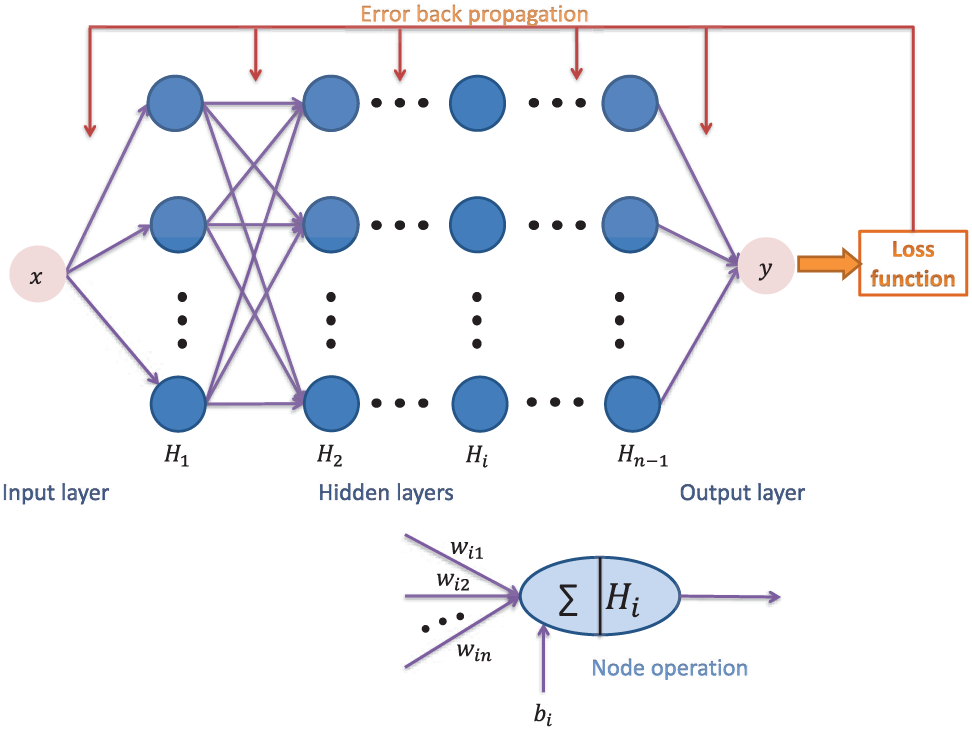
Figure 2: The structure of BPNN

4.2 Construct the Loss Function

Loss function is the most basic element in the neural network. The definition and optimization of the loss function will directly affect the output of the neural network. Therefore, we will realize the simulation of SPD and MFPT by defining different loss functions, and write the simulation results as p^ and T^, respectively. When using the neural network to simulate SPD, we regard the Fokker-Planck equation, the normalization condition and the boundary condition as the governing conditions in the loss function, and the penalty factors aj(1≤j≤3) are introduced to adjust the weight of each governing equation in the loss function. Correspondingly, the loss function can be described as follows:

LSPD=a1∗part1+a2∗part2+a3∗part3,(48)

where

part1=1N⋅∑i=1N|κ1(p^(xΩi,Θ))|2,(49)

part2=|∑i=1NΔx⋅p^(xΩi,Θ)−1|2,(50)

part3=|p^(x2,Θ)|2.(51)

For the case of using neural network to simulate MFPT, the backward Kolomogorov Eq. (25) and the corresponding boundary conditions Eq. (26) are considered as the governing conditions with penalty factors aj(4≤j≤6), so the corresponding loss function is

LMFPT=a4∗part4+a5∗part5+a6∗part6,(52)

where

part4=1N⋅∑i=1N|κ2(T^(xΩi,Θ))|2,(53)

part5=|dT^(x,Θ)dx|x=x1|2,(54)

part6=|T^(x2,Θ)|2,(55)

in which the output T^ of this BPNN is the MFPT for the transition from different tumor densities x to the tumor-present state. Since the main concern of this paper is on the transition from the extinction state to the tumor-present state of the tumor cells, it is sufficient to consider the case x=0 only.

5  Theoretical and BPNN Results

5.1 Effect of the Noises on SPD

The effect of environmental fluctuations on the growth of the tumor cells is an important issue in the study of tumor-immune models. Therefore, in this section, we will analyze the influence of different noise parameters on the tumor by way of the SPDs, and use BPNN to simulate SPDs with the same parametric values as well.

The curves in Fig. 3 describe the changes of SPDs with the different noise parameters. Fig. 3a displays the effect of multiplicative noise intensity D1 on the SPD. It can be found that with the increase of noise intensity D1, the peak value of the SPD curves near x=7.5 gradually decreases, and another peak appears near x=0. In other words, the SPD gradually changes from unimodal to bimodal. Therefore, the fluctuations of external environment have a positive effect on the tumor extinction. In addition, Fig. 3b exhibits that an increase in additive noise intensity D2 will also reduce the peak value near x=7.5 and increase the value near x=0, which means that the internal environment fluctuations promotes the tumor extinction. At last, the increase of the correlation intensity λ will increase the peak near x=7.5. To sum up, internal and external environmental fluctuations can promote tumor extinction, but the interaction between them will inhibit tumor extinction.

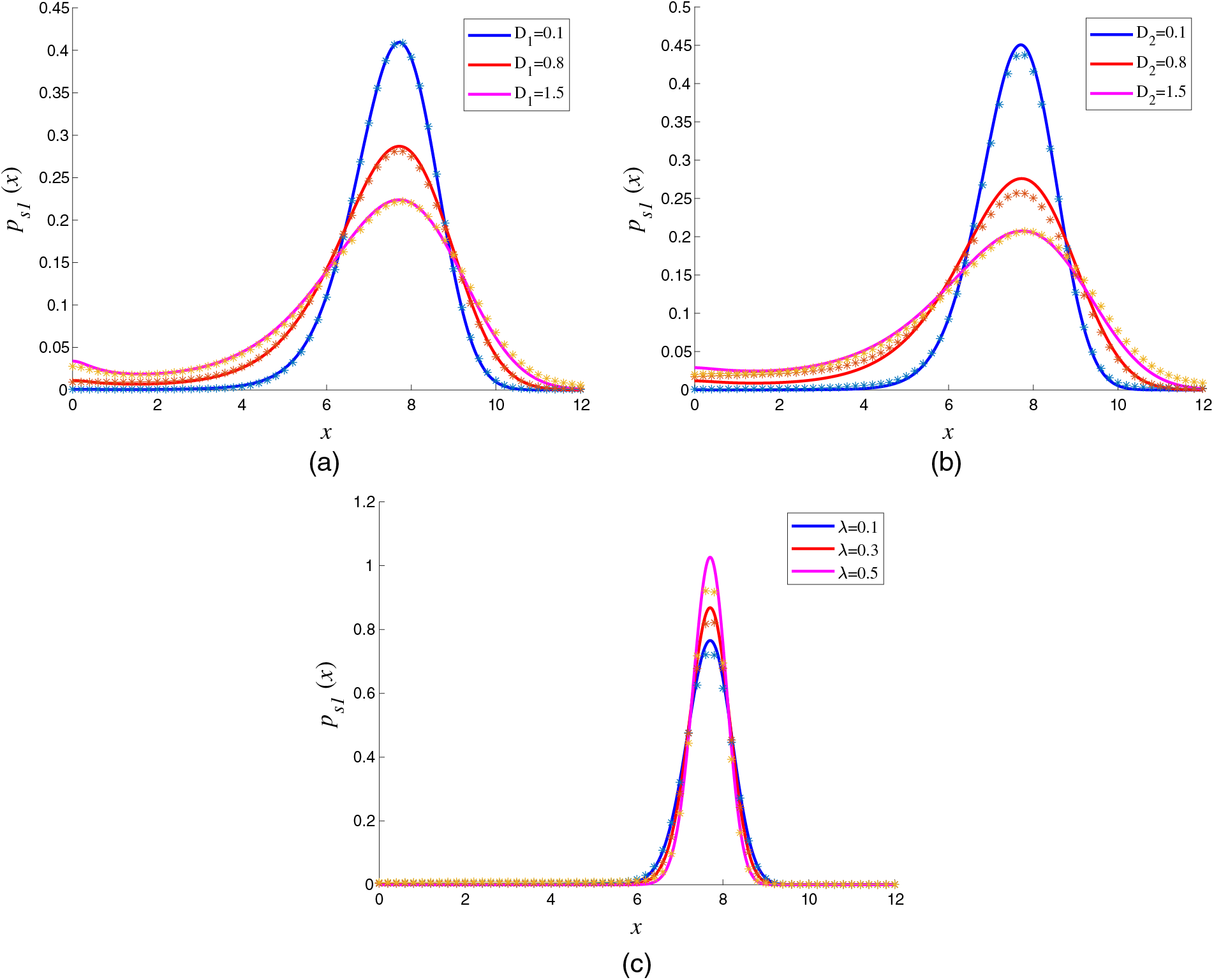
Figure 3: Influence of different noise parameters on SPDs with θ=0.1, β=2.0. Labels: Solid lines, plotted by expression (22); the dots, plotted by BPNN

5.2 Effect of the Noises on MFPT

In addition to the SPD, the performance of the MFPT is also of great significance to the study of tumor immunity, which is a remarkable index to indicate the average transition time from one state to another state. In general, the transition from a steady state to a zero state means that the patient has been cured and the tumor cells are extinct. The transition from a zero state to a steady state, however, means that the tumor has been recurred and the tumor cells appears again. Correspondingly, the knowledge about the recurrence time is especially important for a patient to take all reasonable precaution. Therefore, in this subsection, we will mainly study the effect of environmental fluctuations on the MFPT of the tumor cells from the extinction to the tumor-present state. Based on the theoretical solution of Eq. (28) and neural network solution Eq. (47) for MFPT, Fig. 4 provides the influence of different noise parameters on MFPT.

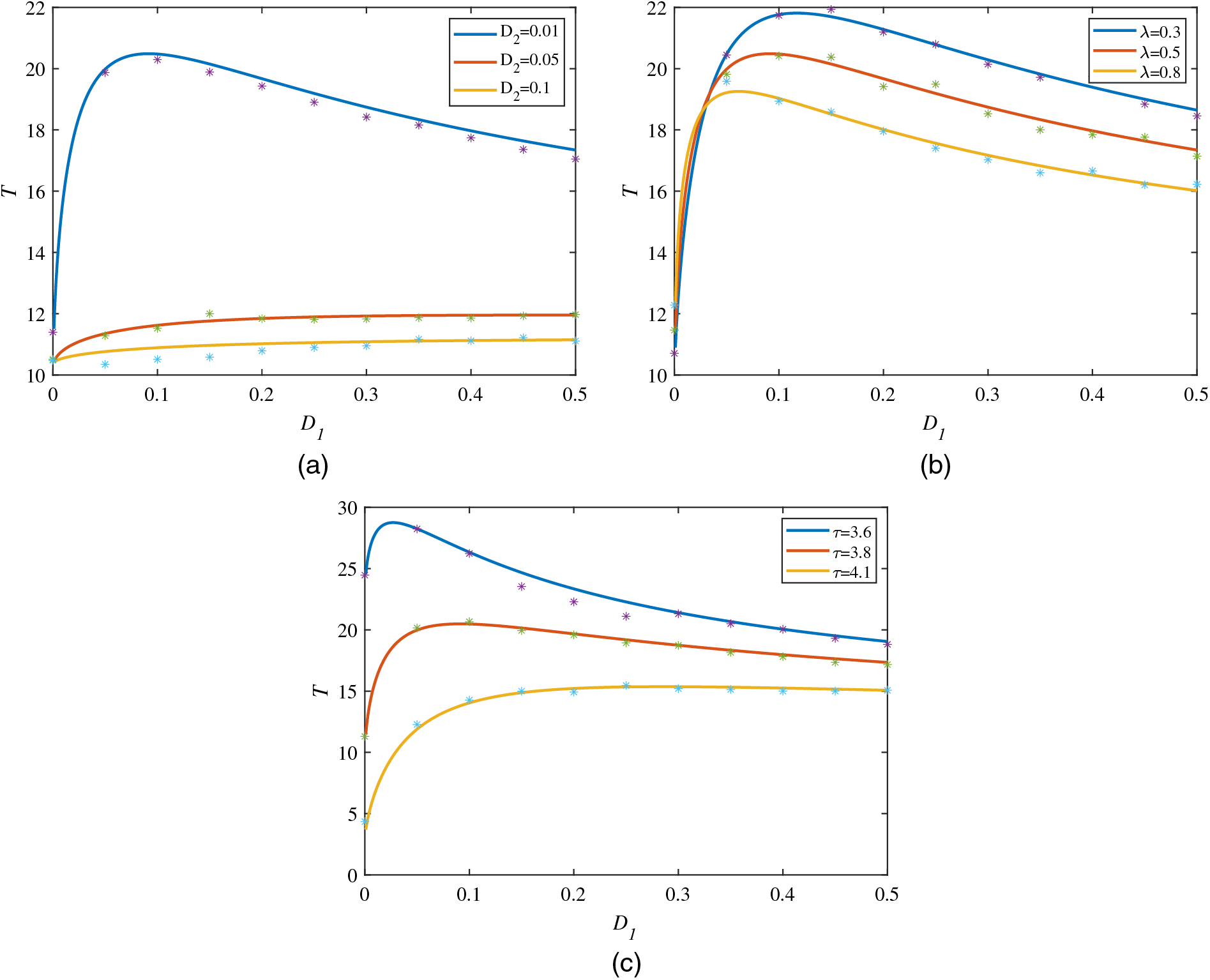
Figure 4: MFPT is a function of D1 under different noise parameters with θ=0.1, β=2.0. Labels: Solid lines, plotted by expression (28); the dots, plotted by BPNN

Firstly, Fig. 4a depicts the change of the MFPT with the intensity of the multiplicative Gaussian colored noise D1 under the different values of the additive Gaussian white noise intensity D2. If D1<0.1, then the smaller value of D2, for example, smaller than 0.1, will increase very fast to a maximal peak, then it will change to decrease with the further increase of D1>0.1. Comparatively, the smaller value of D2<0.1 has a shorter transition time and tends to be unchanged with the value of D1, which means the stronger intensity of white noise is extremely unfavorable to the tumor patients because of the rapid recurrence. Instead, the weak white noise together with weak colored noise is beneficial for prolonging the recurrence time of the tumor. Secondly, Fig. 4b shows the effect of the cross-correlation noise intensity λ of multiplicative Gaussian colored noise and additive Gaussian white noise on the change on the MFPT-D1 plane. It is observed that the increase of the noise correlation intensity λ can significantly reduce the value of resonance-like peak, and the peak position shifts to the left. In addition, with the increase of λ, when D1 is small enough, the corresponding MFPT increases, otherwise it is the opposite. This describes the complex influence of the interaction between internal and external environment on the tumor growth. Finally, through Fig. 4c, we understand the relationship between auto-correlation time τ and MFPT with D1. Observe that the correlation time τ is small enough, the resonance-like peak appears in the MFPT-D1 curves, but disappears when τ increases to 4.1. This phenomenon shows that the increase of correlation time accelerates the recurrence of the tumor cells.

Different from Figs. 4 and 5 mainly describes the influence of the multiplicative noise intensity D1, the across-correlation intensity λ and the correlation time τ on MFPT-D2 plane, respectively. The common feature of all images in Fig. 5 is that when the additive noise intensity D2 is small enough, the MFPT is infinite, and MFPT curves tend to a minimum with the increase of D2. In addition, by observing Figs. 5a and 5b, we can find that the minimum value of the MFPT gradually increases with the increase of the multiplicative noise intensity D1 and the correlation intensity λ. In Fig. 5a, the increase of D1 moves the minimum of the MFPT to the left and increases the corresponding MFPT. Differently, in Fig. 5b, the increase of λ moves the minimum MFPT to the right. In comparison, D1 has a more obviously impact on the MFPT. In other words, the fluctuations of external environment and the interaction between internal and external will inhibit the tumor recurrence, but the individual effect of the external environment fluctuations is more direct and significant. Except that, the effect of the correlation time τ is considered through Fig. 5c. With the gradual increase of τ, the minimum value of the MFPT gradually decreases and moves to the left. The results show that the related time τ can be also accelerate the recurrence of the tumor cells.

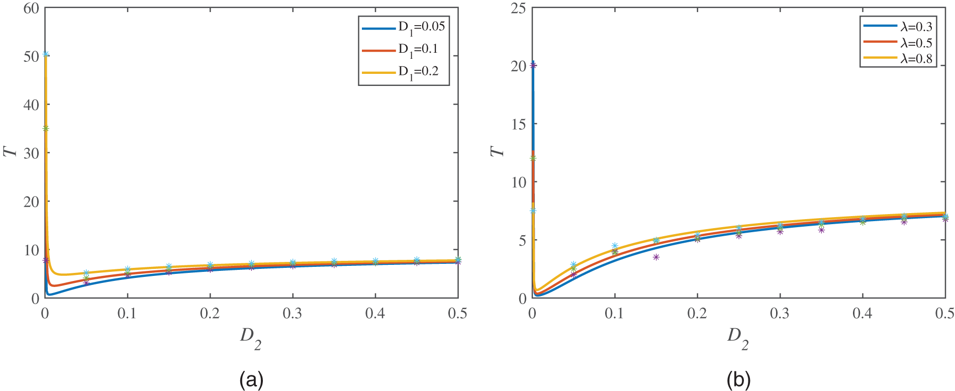
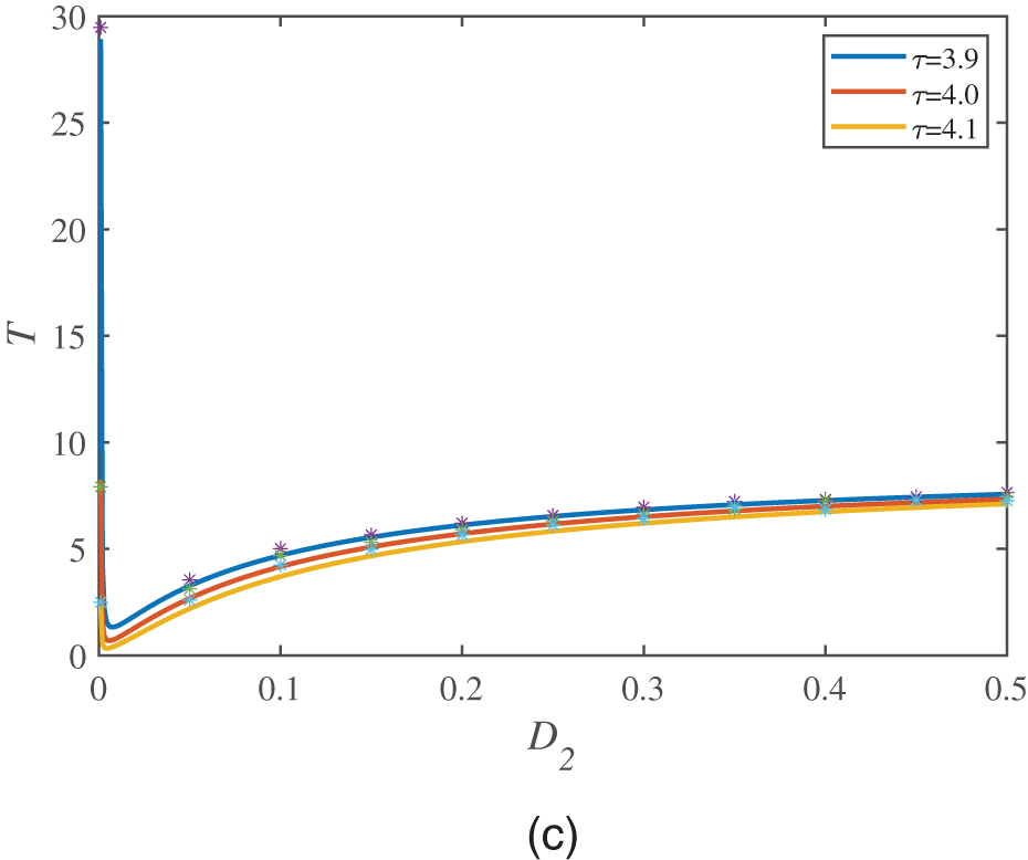
Figure 5: MFPT is a function of D2 under different noise parameters with θ=0.1, β=2.6. Labels: Solid lines, plotted by expression (28); the dots, plotted by BPNN

At the end of this section, we discuss the relationship between the MFPT and the correlation time τ under the different noise parameters. Fig. 6 shows the same tendency is that all MFPTs monotonously decrease with the increase of the correlation time τ, and the decreasing speed gradually slows down. What the differences are, When τ is smaller together with the larger noise parameters, the smaller the MFPT is. However, when the value of τ increases beyond a certain value τc, the influence of the noise parameters on the MFPT have an oppositely change. That is, the bigger noise intensities can have the bigger MFPTs instead. This phenomenon shows that in the process of increasing correlation time τ, the effects of internal and external environmental fluctuations and their interaction on the tumor growth is almost the same, which is firstly supported and then inhibited to make recurrence of the tumors.

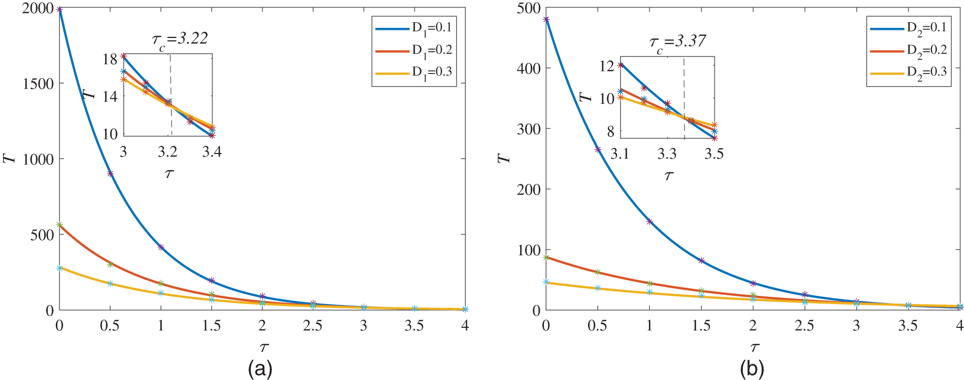
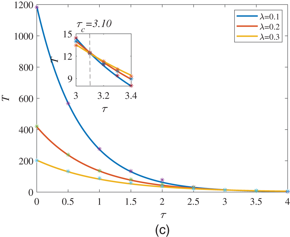
Figure 6: MFPT is a function of τ under different noise parameters with θ=0.1, β=2.6. Labels: Solid lines, plotted by expression (28); the dots, plotted by BPNN

5.3 Effect on SNR

Fig. 7a shows the variation of the SNR with the multiplicative noise intensity D1 and the correlation time τ. We can find that the SNR has an obvious peak with the increase of the noise intensity D1. In the process of τ increasing, the peak value of the SNR at first decreases slightly and then increases significantly, and the corresponding noise intensity D1 decreases gradually when the resonance peak appears. This shows that when the additive noise intensity D2 and the correlation strength λ are 1.0 and 0.5, respectively, the larger correlation time τ can strengthen the SR. According to the Fig. 7b, it can be found that with the increase of the noise intensity D2, the SNR increases briefly, and then begins to decrease rapidly. Therefore, it is obvious that the intensity of the additive noise will also induce the occurrence of the SR. In addition, when both D1 and λ are taken as 0.5, the peak of the SNR will increase with the increase of τ. Therefore, the correlation time τ plays a positive role in stochastic resonance in this case. Fig. 7c introduces the influence of the noise correlation intensity λ and the correlation time τ on the SNR. The main performance is that the resonance peak of the SNR activated by λ gradually moves to the smaller position of λ with the increase of τ until it disappears. If correlation time τ continues to increase, the SNR curve will have a minimal value. This result shows that when the noise intensity D1 and D2 are taken 2 and 3, respectively, the correlation time can significantly inhibit the SR.

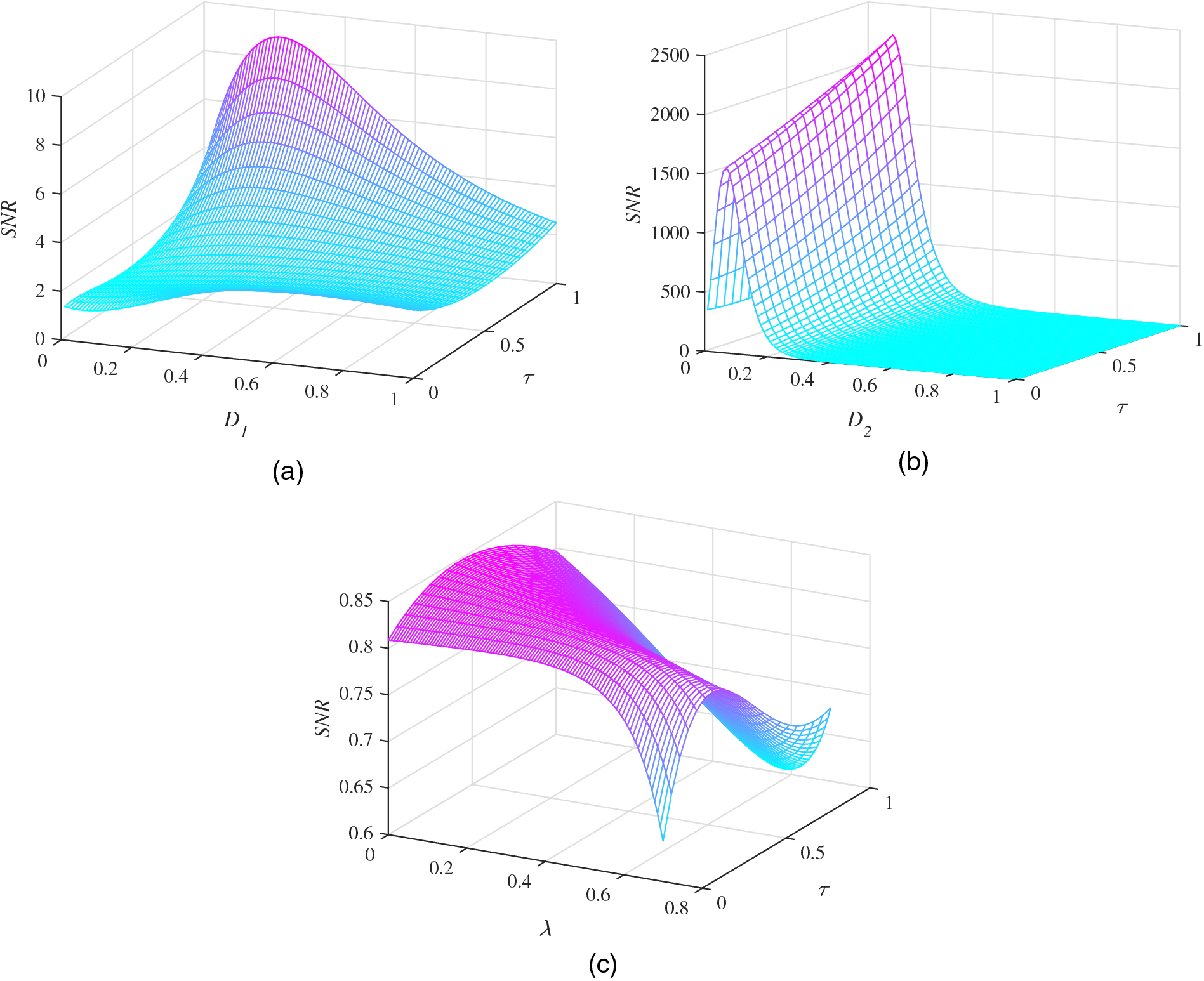
Figure 7: SNR performance under the influence of different noise parameters with θ=0.1, β=2.0

6  Discussion on Optimal BPNN Structure

In this section, our main work is to analyze the feasibility and effectiveness of using BPNN to simulate MFPT. There are three main factors affecting the simulation effect of the neural network, which are the number of hidden layers, the number of nodes in each hidden layer and the value of penalty factors in the loss function. In addition, in order to better show the simulation effect of BPNN on MFPT, we determine that the parameter values in model Eq. (6) are D1=0.1, D2=0.1, θ=0.1, β=2.0 and τ=0.1, respectively. Next, we will discuss the influence of these three factors on the performance of BPNN one by one.

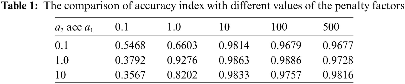
Firstly, the penalty factors can adjust the proportion of different control conditions in the loss function. So it is necessary to discuss the values of the best penalty factors in the loss function LMFPT for model Eq. (6). In order to quantify the accuracy of simulation results, we consider defining an accuracy index acc, which describes the similarity between simulation results T^(x) and accurate results T(x). The acc is written as follows:

acc=1−‖T^(x)−T(x)‖2‖T(x)‖2,(56)

where ‖‖2 denotes the L2 norm.

Table 1 indicates that when a2 is taken as 1.0, the accuracy index acc of BPNN generally performs well. At the same time, as a1 increases from 0.1 to 100, the value of acc also increases, but when a1 increases to 500, the value of acc begins to decrease. Finally, combined with the effects of a1 and a2 on acc, we define the value of loss factors in the BPNN as a1=100, a2=1.0.

Secondly, the number of hidden layers and the number of nodes in the hidden layers determine the structure of the neural network, and their influence on the operation efficiency and accuracy of the neural network is also very important. In order to select the optimal number of hidden layers and nodes, we consider their impact on the performance of the loss function. From Fig. 8, we can find that in the process of gradually increasing the number of hidden layers of BPNN from 1 to 4, the loss function generally decreases first and then increases. And more hidden layers will make the performance of the loss function no longer stable. When the number of hidden layers reaches 3, the loss function will vibrate obviously. Considering the size and stability of the loss function, we judge that the two hidden layers are the best choice.

Figure 8: The comparison of loss functions with different number of hidden layers

Finally, Fig. 9 describes the influence of the number of nodes in the BPNN hidden layer on the neural network simulation results. We find that, compared with the number of hidden layers, the number of nodes has less effect on the performance of the loss function. However, as the number of nodes in each layer increases from 5 to 20, the loss function decreases first and then increases. When the number of nodes is 10, the loss function is reduced to the minimum value, and the performance is more stable with the increase of the number of iterations. In addition, when the number of nodes in the hidden layer is 10, the simulation efficiency of the BPNN is also high. Therefore, for this model, we select the number of nodes in the hidden layer to be 10.

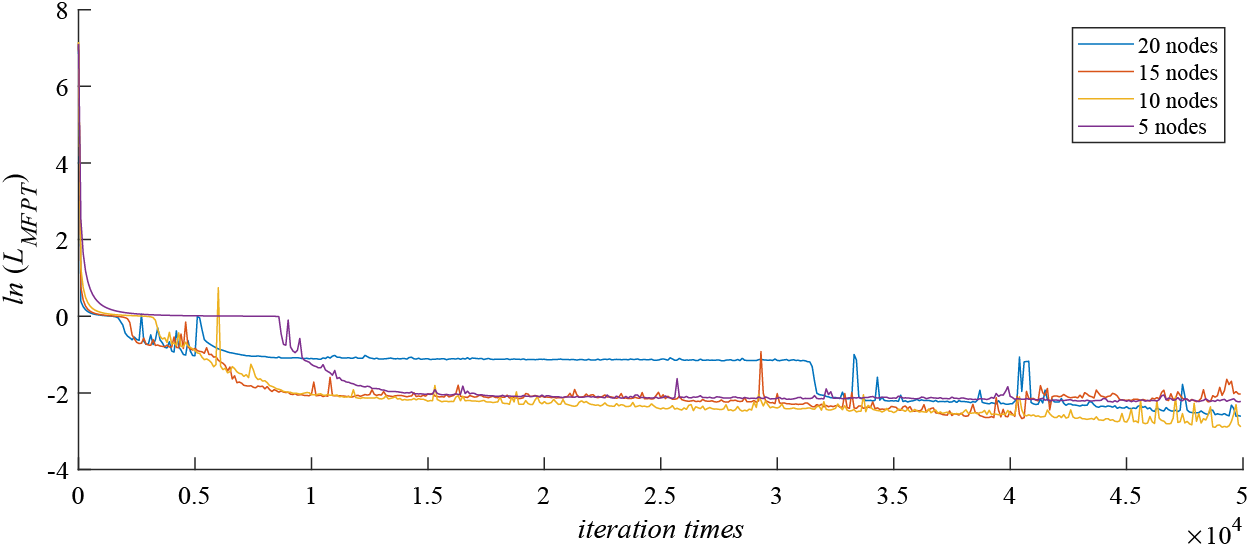
Figure 9: The comparison of loss functions with different number of nodes

To sum up, through the discussion of the experimental results, we have obtained the optimal loss function and neural network structure for the tumor-immune model as n=2, m=10, a1=100 and a2=1. Now, we consider simulating a group of MFPT curves as shown in Fig. 10 to prove the feasibility and effectiveness of BPNN under these parameters. We found that the error of simulation results of BPNN for MFPT fluctuated continuously when the value of D2 increased from 0.1 to 0.3. Although the simulation results of BPNN are always larger and smaller than the exact solutions, but generally, the error value would not exceed 0.1. The result is satisfactory.

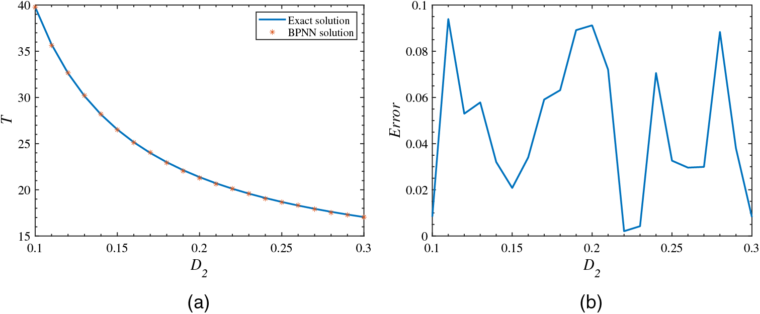
Figure 10: Accuracy diagram of BPNN simulation results

7  Conclusions

In conclusion, this paper focuses on the dynamic properties of the stochastic tumor-immune model perturbed by multiplicative Gaussian colored noise and additive Gaussian white noise, including the effects of noise parameters on SPD, MFPT and SR. Firstly, the expressions of SPD and MFPT were obtained by using the generalized potential function. Then, using the escape rates of tumor cells between the extinction and the tumor-present state, we obtained the exact solution of SNR which was the most representative index of SR. These results showed that in this model, the influence of noise intensity and correlation time on MFPT was complex and diverse. The possibility of tumor recurrence could not be simply controlled by a certain noise parameter. For example, in a smaller correlation time τ, the increase of noise intensity would accelerate tumor recurrence, and in a larger correlation time τ, the opposite was true. About SNR, we found that both noise intensities and correlation intensity could induce the occurrence of SR phenomenon in the model. In contrast, the resonance peak excited by additive Gaussian white noise was the largest. In addition, in order to optimize the simulation effect of BPNN on MFPT introduced in this paper, we also discussed the number of hidden layers, the number of nodes in the hidden layer and the penalty factor in the loss function of BPNN in order to get satisfactory results.

Acknowledgement: The authors wish to express their appreciation to the reviewers for their helpful suggestions which greatly improved the presentation of this paper.

Funding Statement: This work was supported by National Natural Science Foundation of China (Nos. 12272283, 12172266).

Author Contributions: The authors confirm contribution to the paper as follows: study conception and design: Ying Zhang, Wei Li, Guidong Yang, Snezana Kirin; data collection: Ying Zhang, Guidong Yang; analysis and interpretation of results: Wei Li, Snezana Kirin; draft manuscript preparation: Ying Zhang, Wei Li. All authors reviewed the results and approved the final version of the manuscript.

Availability of Data and Materials: The datasets generated during the current study are not publicly available but are available from the corresponding author.

Conflicts of Interest: The authors declare that they have no conflicts of interest to report regarding the present study.

References

1. Leschiera, E., Lorenzi, T., Shen, S., Almeida, L., Audebert, C. (2022). A mathematical model to study the impact of intra-tumour heterogeneity on anti-tumour CD8+ T cell immune response. Journal of Theoretical Biology, 538, 111028. [Google Scholar] [PubMed]

2. Das, P., Das, P., Mukherjee, S. (2020). Stochastic dynamics of Michaelis–Menten kinetics based tumor-immune interactions. Physica A, 541, 123603. [Google Scholar]

3. Chen, Z. H., Zha, H. J., Shu, Z. Q., Ye, J. Y., Pan, J. J. (2022). Assess medical screening and isolation measures based on numerical method for COVID-19 epidemic model in Japan. Computer Modeling in Engineering & Sciences, 130(2), 841–854. https://doi.org/10.32604/cmes.2022.017574 [Google Scholar] [CrossRef]

4. Hao, M., Jia, W., Wang, L., Li, F. (2022). Most probable trajectory of a tumor model with immune response subjected to asymmetric Lévy noise. Chaos Solitons Fractals, 165, 112765. [Google Scholar]

5. Rihan, F. A., Udhayakumar, K. (2023). Fractional order delay differential model of a tumor-immune system with vaccine efficacy: Stability, bifurcation and control. Chaos Solitons Fractals, 173, 113670. [Google Scholar]

6. Atuegwu, N. C., Arlinghaus, L. R., Li, X., Chakravarthy, A. B., Abramson, V. G. et al. (2013). Parameterizing the logistic model of tumor growth by DW-MRI and DCE-MRI data to predict treatment response and changes in breast cancer cellularity during neoadjuvant chemotherapy. Translational Oncology, 6(3), 256–264. [Google Scholar] [PubMed]

7. Patmanidis, S., Charalampidis, A. C., Kordonis, I., Mitsis, G. D., Papavassilopoulos, G. P. (2017). Comparing methods for parameter estimation of the Gompertz tumor growth model. IFAC-PapersOnLine, 50(1), 12203–12209. [Google Scholar]

8. Liao, T. (2022). The impact of plankton body size on phytoplankton-zooplankton dynamics in the absence and presence of stochastic environmental fluctuation. Chaos Solitons Fractals, 154, 111617. [Google Scholar]

9. Qi, H., Meng, X. (2021). Mathematical modeling, analysis and numerical simulation of HIV: The influence of stochastic environmental fluctuations on dynamics. Mathematics and Computers in Simulation, 187, 700–719. [Google Scholar]

10. Deng, Y., Liu, M. (2020). Analysis of a stochastic tumor-immune model with regime switching and impulsive perturbations. Applied Mathematical Modelling, 78, 482–504. [Google Scholar]

11. Fiasconaro, A., Ochab-Marcinek, A., Spagnolo, B., Gudowska-Nowak, E. (2008). Monitoring noise-resonant effects in cancer growth influenced by external fluctuations and periodic treatment. European Physical Journal B, 65(3), 435–442. [Google Scholar]

12. Yin, A., Moes, D. J. A., van Hasselt, J. G., Swen, J. J., Guchelaar, H. J. (2019). A review of mathematical models for tumor dynamics and treatment resistance evolution of solid tumors. CPT: Phamacometrics and System Phamacology, 8(10), 720–737. [Google Scholar]

13. Fiasconaro, A., Spagnolo, B., Ochab-Marcinek, A., Gudowska-Nowak, E. (2006). Co-occurrence of resonant activation and noise-enhanced stability in a model of cancer growth in the presence of immune response. Physical Review E, 74(4), 041904. [Google Scholar]

14. Li, D., Xu, W., Sun, C., Wang, L. (2012). Stochastic fluctuation induced the competition between extinction and recurrence in a model of tumor growth. Physics Letter A, 376(22), 1771–1776. [Google Scholar]

15. Ochab-Marcinek, A., Fiasconaro, A., Gudowska-Nowak, E., Spagnolo, B. (2006). Coexistence of resonant activation and noise enhanced stability in a model of tumor-host interaction: Statistics of extinction times. Acta Physica Polonica B, 37, 1651–1666. [Google Scholar]

16. Han, P., Xu, W., Wang, L., Zhang, H., Ma, S. (2020). Most probable dynamics of the tumor growth model with immune surveillance under cross-correlated noises. Physica A, 547, 123833. [Google Scholar]

17. Li, W., Zhang, Y., Huang, D., Rajic, V. (2022). Study on stationary probability density of a stochastic tumor-immune model with simulation by ANN algorithm. Chaos Solitons Fractals, 159, 112145. [Google Scholar]

18. Hua, M., Wu, Y. (2022). Transition and basin stability in a stochastic tumor growth model with immunization. Chaos Solitons Fractals, 111953. [Google Scholar]

19. Jiang, Y. (2015). A new analysis of stability and convergence for finite difference schemes solving the time fractional Fokker–Planck equation. Applied Mathematical Modelling, 39(3), 1163–1171. [Google Scholar]

20. Sepehrian, B., Radpoor, M. K. (2015). Numerical solution of non-linear Fokker–Planck equation using finite differences method and the cubic spline functions. Applied Mathematics and Computation, 262, 187–190. [Google Scholar]

21. Mulakala, C., Kaznessis, Y. N. (2009). Path-integral method for predicting relative binding affinities of protein-ligand complexes. Journal of the American Chemical Society, 131(12), 4521–4528. [Google Scholar] [PubMed]

22. Sun, Z., Carrillo, J. A., Shu, C. W. (2018). A discontinuous Galerkin method for nonlinear parabolic equations and gradient flow problems with interaction potentials. Journal of Computational Physics, 352, 76–104. [Google Scholar]

23. Zheng, Y., Li, C., Zhao, Z. (2010). A fully discrete discontinuous galerkin method for nonlinear fractional Fokker-Planck equation. Mathematical Problems in Engineering, 2010, 279038. [Google Scholar]

24. Bararnia, H., Esmaeilpour, M. (2022). On the application of physics informed neural networks (PINN) to solve boundary layer thermal-fluid problems. International Communications in Heat and Mass Transfer, 132, 105890. [Google Scholar]

25. Santosh, T., Soni, R. K., Eswaraiah, C., Kumar, S. (2022). Application of artificial neural network method to predict the breakage properties of PGE bearing chromite ore. Advanced Powder Technology, 33(3), 103450. [Google Scholar]

26. Li, S., Yang, Y. (2021). A recurrent neural network framework with an adaptive training strategy for long-time predictive modeling of nonlinear dynamical systems. Journal of Sound and Vibration, 506, 116167. [Google Scholar]

27. Li, D., Xu, W., Guo, Y., Xu, Y. (2011). Fluctuations induced extinction and stochastic resonance effect in a model of tumor growth with periodic treatment. Physics Letters A, 375(5), 886–890. [Google Scholar]

28. Shi, P., Xia, H., Han, D., Fu, R., Yuan, D. (2018). Stochastic resonance in a time polo-delayed asymmetry bistable system driven by multiplicative white noise and additive color noise. Chaos Solitons Fractals, 108, 8–14. [Google Scholar]

29. Guo, Y., Yao, T., Wang, L., Tan, J. (2021). Lévy noise-induced transition and stochastic resonance in a tumor growth model. Applied Mathematics Modelling, 94, 506–515. [Google Scholar]

30. Cao, L., Wu, D. J., Ke, S. Z. (1995). Bistable kinetic model driven by correlated noises: Unified colored-noise approximation. Physical Review E, 52(3), 3228. [Google Scholar]

31. Wu, J. L., Duan, W. L., Luo, Y., Yang, F. (2020). Time delay and non-Gaussian noise-enhanced stability of foraging colony system. Physica A, 553, 124253. [Google Scholar]

32. Jia, Y., Yu, S. N., Li, J. R. (2000). Stochastic resonance in a bistable system subject to multiplicative and additive noise. Physical Review E, 62(2), 1869–1878. [Google Scholar]

33. Cheng, G., Liu, W., Gui, R., Yao, Y. (2020). Sine-wiener bounded noise-induced logical stochastic resonance in a two-well potential system. Chaos Solitons Fractals, 131, 109514. [Google Scholar]

34. Wang, B., Gao, F., Gupta, M. K., Królczyk, G., Gardoni, P. et al. (2022). Risk analysis of a flywheel battery gearbox based on optimized stochastic resonance model. Journal of Energy Storage, 52, 104926. [Google Scholar]

35. Yamazaki, H., Lioumis, P. (2022). Stochastic resonance at early visual cortex during figure orientation discrimination using transcranial magnetic stimulation. Neuropsychologia, 168, 108174. [Google Scholar] [PubMed]

36. Zhou, Z., Yu, W., Wang, J., Liu, M. (2022). A high dimensional stochastic resonance system and its application in signal processing. Chaos Solitons Fractals, 154, 111642. [Google Scholar]

37. Jiao, S., Gao, R., Zhang, D., Wang, C. (2022). A novel method for UWB weak signal detection based on stochastic resonance and wavelet transform. Chinese Journal of Physics, 76, 79–93. [Google Scholar]

38. Ning, L. J., Xu, W., Yang, X. L. (2007). The mean first-passage time for an asymmetric bistable system driven by multicative and additive noise with colored correlations. Acta Physical Sinica, 56(1), 25–29. [Google Scholar]

39. Zan, W., Xu, Y., Metzler, R., Kurths, J. (2021). First-passage problem for stochastic differential equations with combined parametric gaussian and lévy white noises via path integral method. Journal of Computational Physics, 435, 110264. [Google Scholar]

40. Yin, H., Wen, X. (2019). First passage times and minimum actions for a stochastic minimal bistable system. Chinese Journal of Physics, 59, 220–230. [Google Scholar]

41. Boehm, U., Cox, S., Gantner, G., Stevenson, R. (2021). Fast solutions for the first-passage distribution of diffusion models with space-time-dependent drift functions and time-dependent boundaries. Journal of Mathematical Psychology, 105, 102613. [Google Scholar]

42. Hohenegger, C., Durr, R., Senter, D. (2017). Mean first passage time in a thermally fluctuating viscoelastic fluid. Journal of Non-Newtonian Fluid Mechanics, 242, 48–56. [Google Scholar]

43. Wei, J. L., Wu, G. C., Liu, B. Q., Zhao, Z. G. (2022). New semi-analytical solutions of the time-fractional Fokker-Planck equation by the neural network method. Optik, 168896. [Google Scholar]

44. Guo, X., Zhang, Y. D., Lu, S., Lu, Z. (2022). A survey on machine learning in COVID-19 diagnosis. Computers, Materials & Continua, 130(1), 23–71. https://doi.org/10.32604/cmes.2021.017679 [Google Scholar] [CrossRef]