Examining the Use of Scott’s Formula and Link Expiration Time Metric for Vehicular Clustering

1  Introduction

In a vehicular network (VN) environment, clustering refers to organizing vehicles into groups based on their geographical location or other shared characteristics. Clustering can improve vehicle communication, data exchange and facilitate coordinating activities such as traffic control and emergency response. Moreover, clustering can improve routing scalability and reliability in VN [1]. Some common methods for clustering in a VN environment include distance-based, density-based, and connectivity-based clustering [1]. The ad-hoc nature of VN dictates the clustering process to be distributed among the vehicles through a self-election process to select Cluster Head (CH) and Cluster Members (CM) [2]. However, using Machine Learning (ML) algorithms for clustering may not be feasible without the road infrastructure to provide more features and reduce the vehicle’s workload [3]. Therefore, adapting ML clustering algorithms to fit the VN environment is essential. The original Partitioning Around Medoids (PAM) algorithm involves selecting the initial K medoids in a greedy process (BUILD stage) that minimizes the sum of dissimilarities or total deviation (TD) [4]. The BUILD stage version presented in [5] caches the dissimilarity value to the nearest medoid to reduce the time complexity to O(N 2K). The second stage of the algorithm, the SWAP stage, optimizes the initial selection and chooses alternative medoids that reduce the change in TD. Two improved versions of the SWAP stage were presented in [5] that eliminate the nested K iterations and reduce the redundancy of calculating the TD for every possible swap of medoids. The time complexity of the SWAP stage O(K(N-K) 2) was reduced to O(N(N-K)) with these improvements. Instead of the greedy process, the K-Medoids algorithm randomly selects the initial medoids, just like Lloyd’s algorithm. Moreover, the K-Medoids algorithm follows the naive implementation of precomputing the dissimilarity matrix and calculating the TD for every possible swap [6].

The PAM and K-Medoids algorithms are written with dissimilarity metrics such as the Euclidean distance in mind. However, as shown in previous work [7], similarity metrics such as the Link Expiration Time (LET) [8] can work with the K-Medoids algorithm by maximizing the TD instead of minimizing it. The LET equation combines distance, speed, direction, and communication range to calculate the connection period between two vehicles, which makes it excellent for clustering vehicles. Moreover, the LET equation was driven mathematically and validated for highway scenarios by [9]. However, selecting the correct number of clusters is essential for effective clustering. Therefore, Scott’s formula was suggested to estimate the K number instead of the Elbow and Silhouette methods for vehicle clustering [7]. Scott’s formula [10] is used to compute the bin numbers for constructing a histogram. Histograms are used to visualize the underlying distribution of a set of numerical data to identify patterns and trends. Therefore, this statistical tool could help to calculate the optimal number of clusters cost-effectively for vehicle clustering.

This work further investigated the possibility of using Scott’s formula to calculate the K number for vehicle clustering and the LET metric as the clustering metric. The FastPAM clustering algorithm [5] was considered because of its quick convergence. In the simulation, vehicle information is recorded by the Road Side Unit (RSU), which builds and updates its neighbor table based on the vehicles’ beacons every time a CH leaves its transmission range, or a new vehicle enters its transmission range. The simulations will be based on three road maps; Highway, Traffic Light junction, and Roundabout junction. The traffic flow for the highway map will be based on a survey by [11]. The traffic flow for the other maps will be based on examples’ values from the Highway Capacity Manual [12,13] to provide realistic simulations. The contributions of this paper are:

• Using the FastPAM algorithm for vehicle clustering.

• Using a negative LET similarity matrix instead of modifying the original clustering algorithm.

• Using realistic traffic flow values for the simulated Highway, Traffic Light junction, and

  Roundabout junction road map scenarios.

The remnant of the paper is laid as follows. The related literature is reviewed in Section 2 with background about the affiliated topics. Section 3 introduces the methodology, while Section 4 presents the simulation process and the results with a discussion. Finally, Section 5 concludes the findings.

2  Background and Related Work

Unsupervised clustering algorithms such as K-Means, K-Medoids, and PAM algorithms require the number of clusters (K) to be known in advance [14]. There are several approaches for estimating the K number for these algorithms, such as the Elbow method, Silhouette analysis, and Gap statistic [15]. The Elbow method involves fitting the clustering model for a range of K values and then plotting the total deviation (TD) for each value of K. The “knee” of the elbow-shaped curve is the point of inflection where the TD begins to level off, and this can be taken as a reasonable estimate for the optimal value of K [16]. There are algorithms to find the “knee” point of the curve relative to a particular sensitivity factor [17]. However, the Elbow method is still considered subjective, as the “knee” point is not always clearly defined and may depend on the interpretation of the person analyzing the plot. Additionally, the elbow method may not always provide a reliable estimate of the optimal value of K, especially if the data do not have a clear underlying structure or if there is much noise [18].

Even though the Silhouette method is used to evaluate the quality of the clustering outcome, it can also give a reasonable estimation of the number of clusters. This method involves computing a silhouette score for each sample, which measures how closely it is matched to its cluster vs. the next best cluster [19]. The value range of the score is between −1 and 1, where values close to (1 or −1) represent distinguishable clusters or wrongly assigned clusters, respectively. However, zero value represents indistinguishable clusters or unclustered points. The optimal value of K is the one that maximizes the mean silhouette score across a sensible range of K [20]. Another alternative to the Silhouette method is the Medoid-Silhouette method which only calculates the score based on the distance to the medoids of the clusters instead of the average distance to all cluster members [21].

The Gap statistic method involves fitting the model for a range of K values and comparing the results to those obtained using a reference distribution, such as a uniform random sample [22]. The optimal value of K is the one that maximizes the gap between the model’s log-likelihood and that of the reference distribution. The above methods are not feasible to pick the K number for an online vehicular clustering algorithm due to the high time complexity requirement of these methods. Moreover, a dataset that cannot produce a reliable random reference distribution, such as the features required for calculating the LET, cannot be used with Gap statistics.

Regarding unsupervised clustering without knowing the K number, the Affinity propagation algorithm implements a message exchange process between the data points until consent for the number of clusters is reached. However, the time complexity of this algorithm is O(N 2T), where T is the number of iterations required for convergence [23]. The DBSCAN needs the epsilon value to be present, which is the maximum distance between two data points for these points to be considered in the neighborhood of each other [24]. Moreover, hierarchical clustering requires a threshold to merge points/clusters into another cluster [25]. Therefore, this work considered the estimated K number by the Affinity propagation algorithm and the Medoid-Silhouette method as a baseline. The latter method was selected as not all the pairwise vehicles in the neighbor table had an LET value because they may not be in communication range.

To avoid computational complexity, the solutions to estimate the K number presented by VN clustering schemes usually rely on the in-range number of vehicles and the covered geography. For example, the road length was divided by multiplying the number of transmission ranges, and the summation of transmission ranges to estimate the K number in [26]. However, the number of transmission ranges was multiplied by the ratio of the road length to the summation of transmission ranges in [27,28] to estimate the K number. The algorithm presented in [29] picks the K number from a maximum function of the road length to transmission range ratio and the number of vehicles to the maximum number of CM ratio. Furthermore, the work in [30] formulated a Maximum Stable Set Problem (MSSP) using the vehicles’ similarity scores and solving it with the Continuous Hopfield Network (CHN) to estimate the K number and select the initial medoids. For single-hop clustering, the authors in reference [31] stated that the covered geography and transmission range are inversely proportional to the cluster size. Therefore, they proposed a brute force method to learn the K number by randomly selecting a CH, assigning the in-range vehicles to it, and then repeating the process for the remaining unassigned vehicles. Finally, the related work above lacks a lightweight and efficient K selection method, which this paper proposes using Scott’s formula.

3  Research Methodology

This section presents the communication and road network models, the clustering metrics, and the assessment process of estimating the K number based on the baselines.

3.1 Communication Model

The communication model is based on the DSRC standard, which expects the vehicles to be equipped with DSRC On-Board Unit (OBU) and a Global Positioning System (GPS) module. According to the SAE J2735 standard, the vehicles broadcast a periodic Basic Safety Message (BSM) that includes its ID (MAC address), position, speed, and heading as an angle. As the previous work [7] presented, two fields are added to the BSM to aid the clustering process. The first field is for the CH ID, and the second one includes the vehicle’s average received power. The CH ID field will help indicate the vehicle’s clustering status, which will be used in future work.

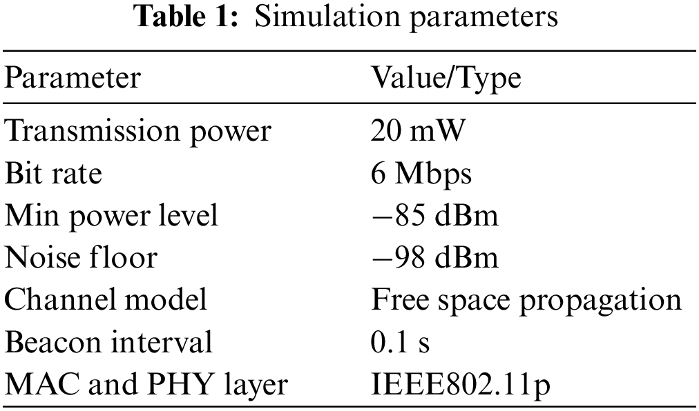
To fill the second additional field, the vehicle registers the recorded power of the received BSMs and averages it over 5 s. Then the average received power is divided by the number of vehicles in the range of the corresponding vehicle. The five-second reset period is chosen to ensure that the average value is recalculated at least three times during the passing of a vehicle traveling at a speed of 120 km/h through the transmission range of the vehicle in question. This metric could quantify the vehicle’s connection with its neighbors. For the rest of the paper, this metric will be referred to as vehicle average received power (VehRxdBm). The model also includes a Road Side Unit (RSU) that gathers the information the vehicles broadcast and forms a neighbor table. Table 1 contains the considered simulation parameters, communication figures, and standards. Both the vehicles and the RSU share the same communication ability in terms of power and transmission range, which is around 300 m, considering the channel propagation model and transmission parameters presented in Table 1.

3.2 Road Network Models and Traffic Flow Values

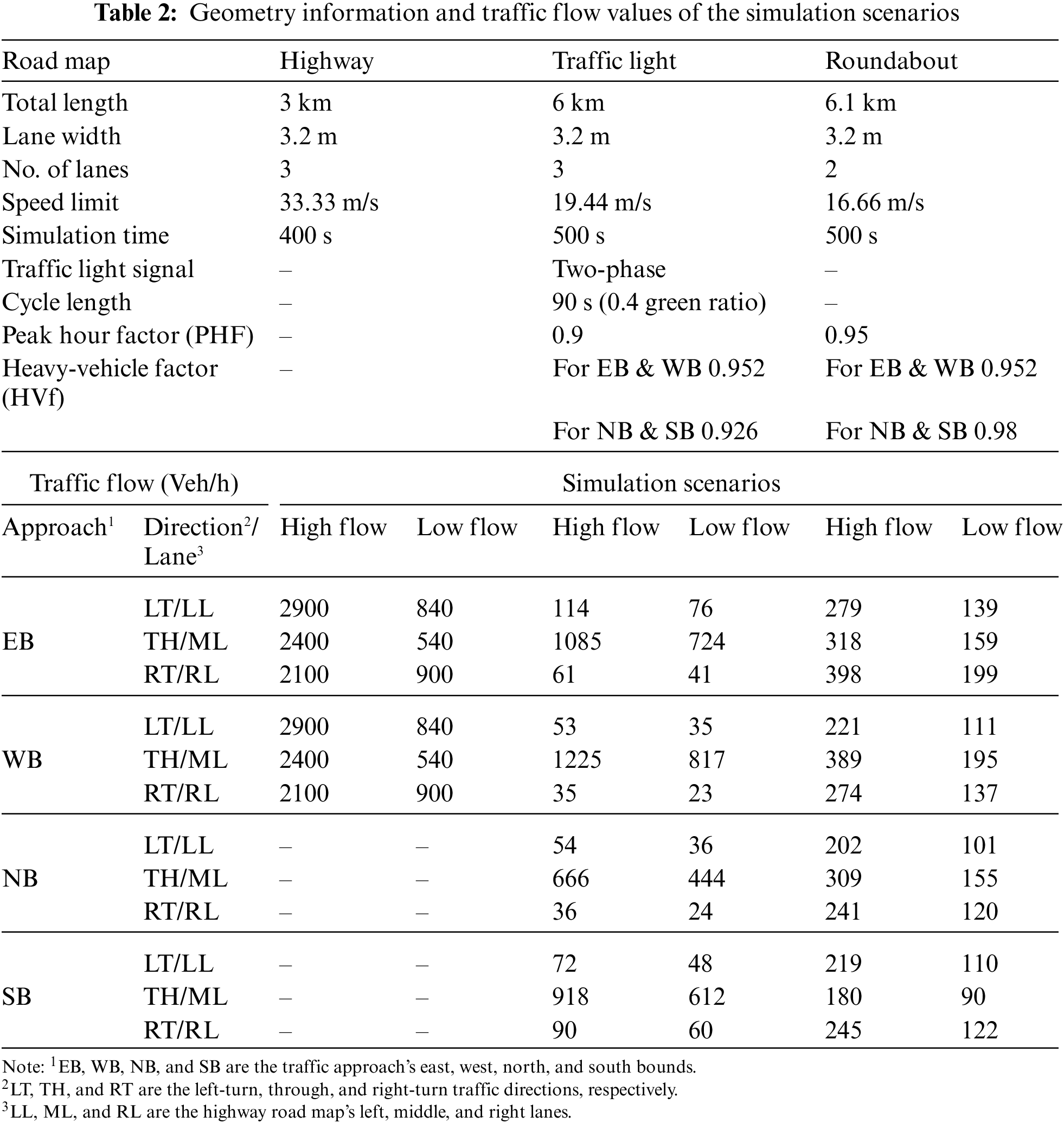
The reviewed vehicle clustering literature simplified their simulations by only considering highway road map scenarios. However, this paper considered three road maps, Highway, Traffic Light junction, and Roundabout junction, to study the effect of road layout on the estimation of K number. Fig. 1 shows the three simulated road maps. Table 2 contains the simulated road maps’ geometry information and traffic flow values. The simulated two-way highway road is 3 km in length with three lanes for each side.

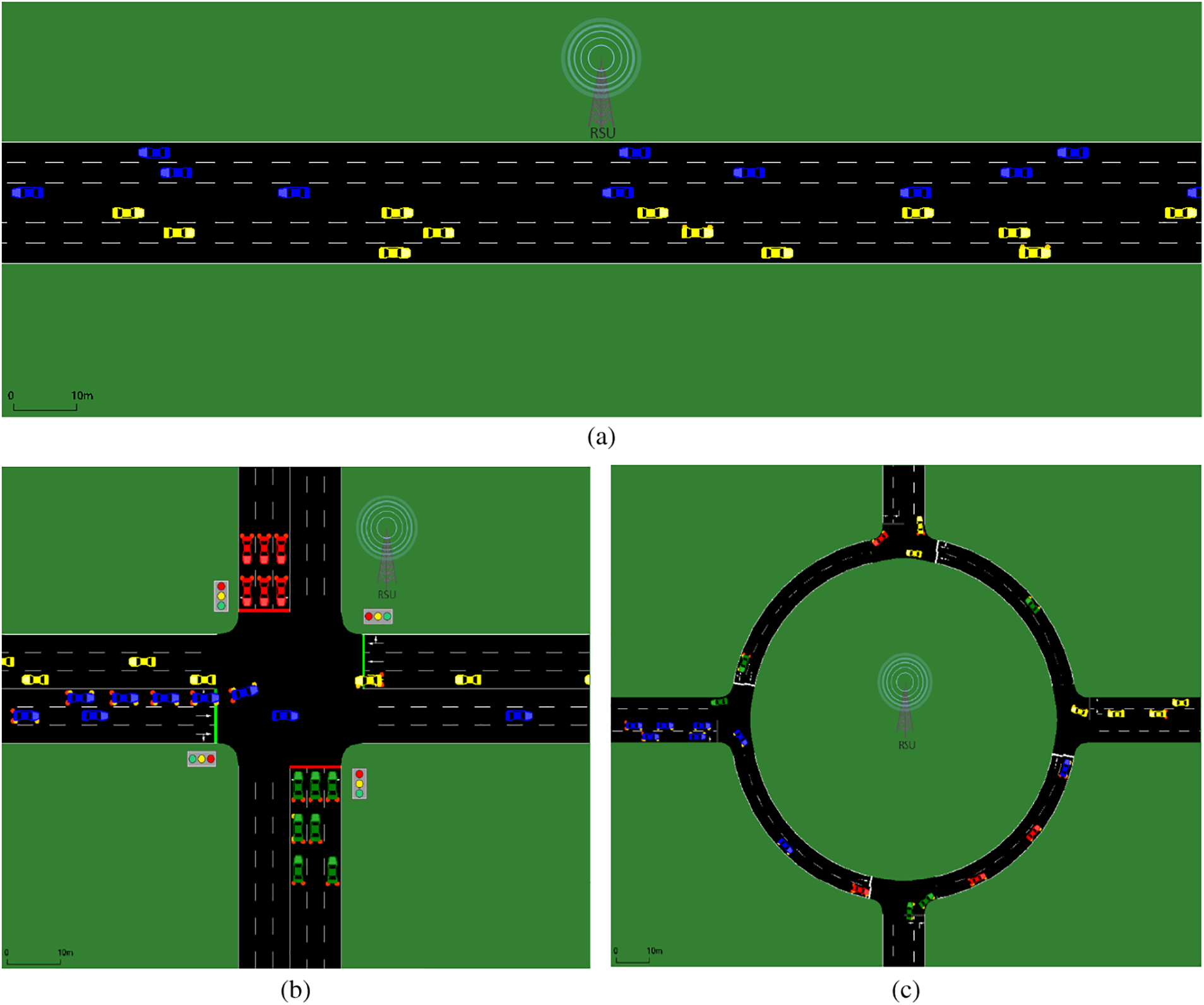
Figure 1: Simulated road maps: (a) three lanes two-way highway; (b) three lanes two-way four-legged traffic light junction; (c) two lanes two-way four-legged roundabout

The Traffic Light junction is a four legs two-way cross junction with three lanes on each side. Each leg of the traffic light junction is 1.5 km long with exclusive left-turn and right-turn lanes. The traffic light cycle is split into 40 s for the green period and 5 s for the red/yellow gap period. For the roundabout layout, a two-way two lanes roundabout intersection is considered with a 91.44 m inscribed circle diameter according to the NCHRP guidelines [32]. The four legs connected to the roundabout with the inscribed circle diameter make 3 km length roads in each direction. The speed limits are set based on the functional and design considerations for highway and urban roads in [12]. The vehicle’s arrival speed in the simulation is set to 5 km/h lower than the road limit to ensure the required traffic flow is reached when the vehicle enters the communication range of the RSU. The simulation time for each map is 300 s plus how long a vehicle would take to cross from one point of the simulated map to the farthest point traveling at the speed limit of the corresponding road map. The calculation included the time lost waiting at the traffic light or crossing the roundabout.

The reviewed literature considered traffic density which refers to the number of vehicles present in a length of a lane or roadway at a given time. Traffic density is typically measured in vehicles per unit of length or area, such as vehicles per kilometer (veh/km) or vehicles per square kilometer (veh/km 2). Measuring density in the field is challenging because it requires a visual vantage point for the road section or area in question [12]. Therefore, this work considered the traffic flow metric, measured in terms of the number of vehicles passing a specific point of the road or lane over a given period, such as the number of vehicles per hour (veh/h). The traffic flow measurement is usually done over 15 min intervals for one hour. The maximum measurement of the four 15 min periods is expressed in hours as the traffic flow for that specific road point.

This paper considered two traffic flow scenarios, high flow (HF) and low flow (LF), for the maps mentioned above. The northbound (NB), southbound (SB), eastbound (EB), and westbound (WB) traffic flow figures shown in (Table 2) are driven from various traffic-related sources and based on the level of service (LOS) analysis. The operation conditions of roads and intersections are quantified with six LOS (A through F), where “A” represents the optimal conditions, and “F” represents the worst conditions [12].

The traffic flow survey for the M60 highway in Manchester city in the UK mentioned and analyzed by [11] (p. 412) is used to set the LF and HF traffic for the simulated highway map. The left-hand UK traffic was considered when using the traffic flow values for the right-hand traffic of the simulated map (Table 2). The low traffic flow scenario for the traffic light junction map is taken from “Problem Example 1” in [12] (p. 16–38). The reason behind this selection was that the LOS analysis of the example was “C”. Therefore, the high-traffic flow scenario is constructed by increasing the flow values of the low-traffic scenario by 50%. Regarding the roundabout map, the traffic flows are driven by guidelines in Exhibit 22–6 of [13] (p. 22–7). The LOS analysis of the low traffic flow values (Table 2) was “A”. Thus, the values of the low traffic flow scenario are doubled to create the high flow scenario. Finally, the traffic flows in Table 2 are the adjusted values by the peak hour factor (PHF) and heavy-vehicle factor (HVf) for the roundabout and traffic light road maps.

3.3 Clustering Metrics and Algorithm

The clustering metrics used with the FastPAM clustering algorithm will be mentioned in this section. Histogram visually summarizes the underlying probability density function of data. This statistical tool visualizes the frequency distribution of the data by classifying the data points into “bins”. These bins hold how many data points of the same range belong to each of these bins. Various formulas calculate the number of bins for histograms [33]. Scott’s formula calculates the number of bins for the histogram by taking the Gaussian density as a reference standard to have a data-based choice for the number of bins [10].

 Bin Number =max(data)−min(data)3.5×stdev⁡(data)n3(1)

The max, min, and stdev are the data’s maximum, minimum, and standard deviation values, respectively, while n is the number of entries in the data. This work evaluated seven inputs for Scott’s Eq. (1) to estimate the K number. The first and second inputs are the vehicles’ X and Y coordinates. The third input is the vehicle’s average received power (VehRxdBm), explained in Section 3.1. The fourth input is the BSM received power recorded by the RSU for each vehicle in its range (RSURxdBm). The fifth input is the distance between each vehicle and the RSU (Dis2RSU). The sixth input is the average distance between each vehicle and the other vehicles in the range of the RSU (AvgDis). The seventh input is the average LET value (AvgLET) for each vehicle computed in reference to the other vehicles in the RSU range.

The novelty of using the LET metric to compute the vehicle similarity score for the K-Medoids algorithm is shown in [7]. However, the past work modified the clustering algorithm because the K-clustering algorithms are written based on the Euclidean distance, a dissimilarity metric. The LET equation returns an infinite or very high number to indicate that the two adjacent vehicles will stay in the communication range for a long time [8]. For two adjacent vehicles, i and j, the LET equation is:

LET=−(ab+cd)+(a2+c2)r2−(ad−bc)2a2+c2(2)

where,

a=vicos⁡θi−vjcos⁡θj,b=xi−xj,c=visin⁡θi−vjsin⁡θj,d=yi−yj.

v is the vehicle’s speed (m/s) and (x,y) its coordinates, while θ is the moving direction in degree. r is the communication range in meters based on the free space propagation model. The FastPAM clustering algorithm is a K-clustering algorithm based on minimizing the TD. Therefore, negative LET values are fed to the algorithm to accommodate the similarity metric, keep the concept of TD minimization, and avoid modifying the clustering algorithm. The use of negative values is a valid and proven method. The affinity propagation algorithm transforms the Euclidean distance-based dissimilarity matrix into a negative values similarity matrix. The maximum distance between vehicles is their communication range. Therefore, the infinity values are replaced with the maximum LET value in the similarity matrix.

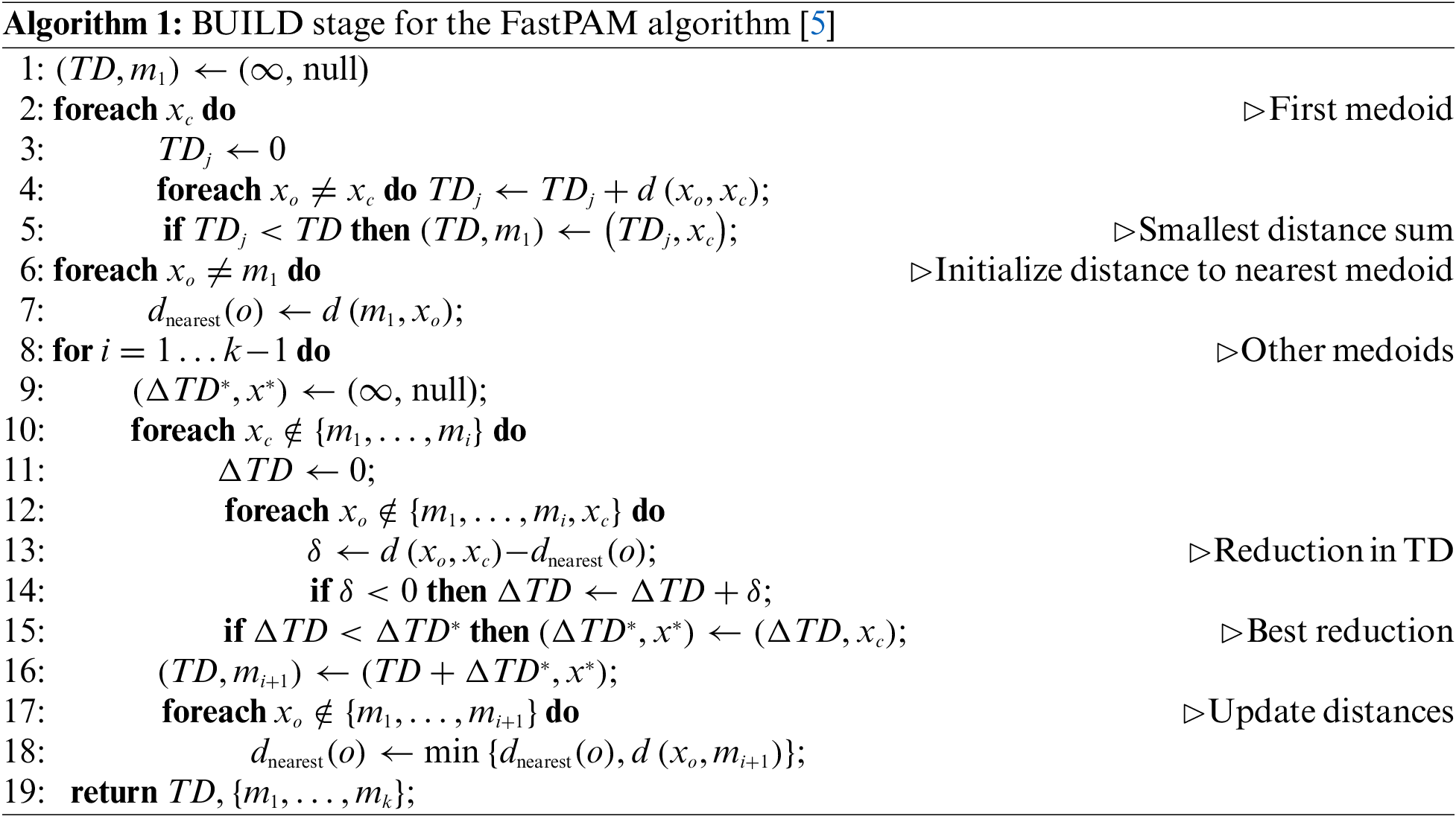
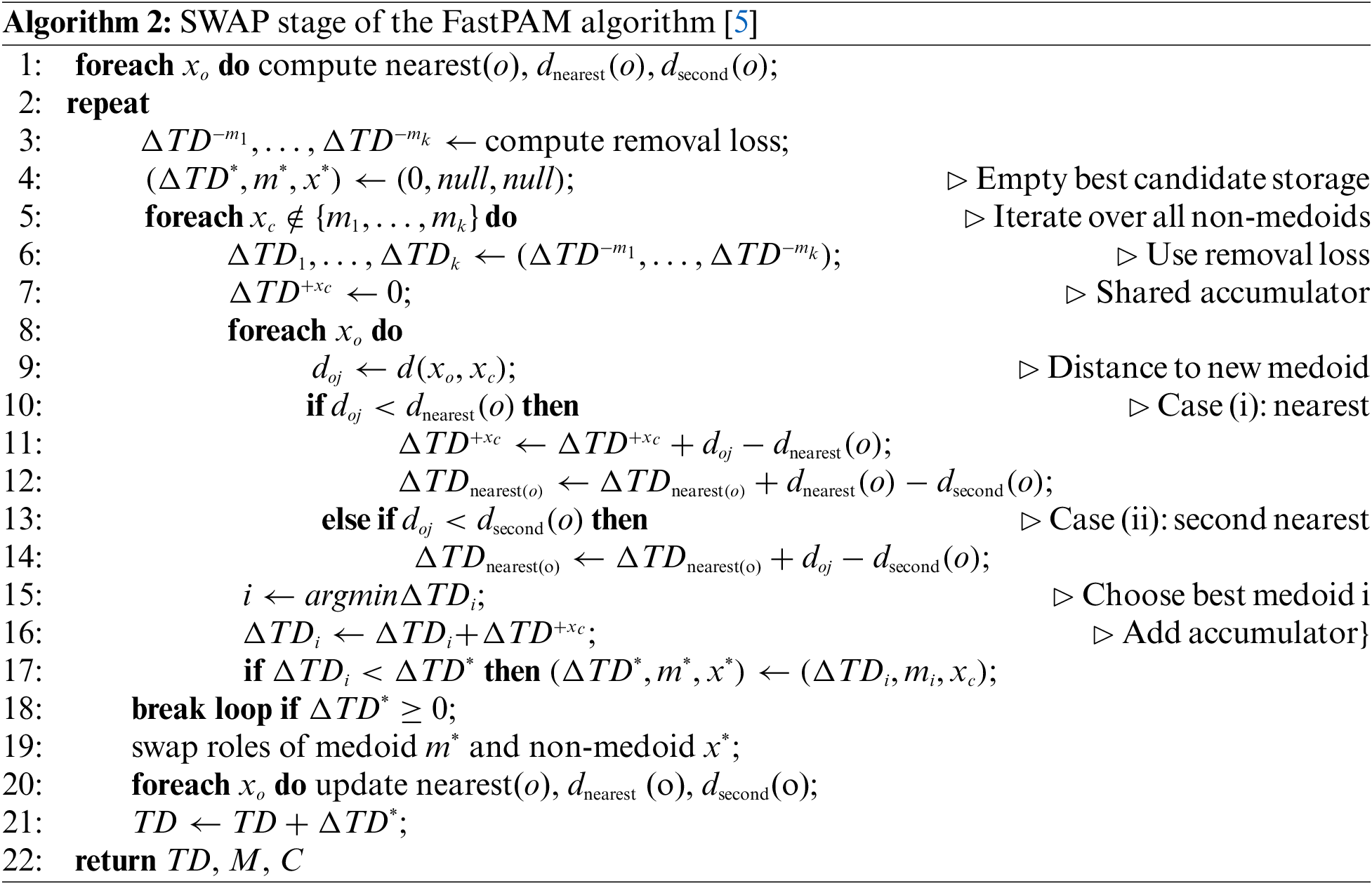
The clustering algorithm used in this work is a modified version of the Partitioning Around Medoids (PAM) algorithm. Algorithms 1 and 2 represent the BUILD and SWAP stages for the FastPAM algorithm [5]. The FastPAM algorithm, like the original PAM, picks the medoids that reduce the change in TD instead of computing the TD at every iteration. The FastPAM uses the original PAM BUILD stage (Algorithm 1), a greedy process to pick the initial medoids according to the provided K number. However, it modifies the SWAP stage (Algorithm 2) to gain faster performance by eliminating the nested K iterations and reducing the redundancy of calculating the TD for every possible swap of medoids. Instead of calculating the TD at every iteration, the algorithm computes the change in TD (ΔTD) for every datapoint (xo) when a selected medoid (mi) is swapped with a candidate medoid (xc). Moreover, the caching of distance to the nearest (dn(o)) and second best (ds(o)) medoids of (o) increase the performance compared to the naive approach of calculating TD at every swap. Furthermore, the ΔTD is decomposed into a positive loss (ΔTD−mi) of reassigning medoid (mi)’s members to the second-best alternative and a negative loss (ΔTD+xc) of reassigning the nearest points to the candidate medoid xc. Information on how to compute these values can be found in [5].

The second contribution mentioned in the previous work [7] is that the BUILD stage can be opted out in favor of selecting the initial medoids base on a vehicle communication metric. Therefore, this work will evaluate the use of the vehicle’s average received power (VehRxdBm) and the average LET value of each vehicle (AvgLET) to pick the initial medoids. A high VehRxdBm could indicate that the vehicle is connected to numerous other vehicles, while a high AvgLET could suggest that the vehicle has a solid connection to its neighbors. The LET metric (2) incorporates the vehicle coordinates, speed, and moving direction, making it comprehensive. The vehicle’s distance from the RSU and the other vehicles can not indicate how well the vehicle is connected to its neighbors. Moreover, how well the vehicle is connected to the RSU can not be used as a metric for selecting the initial medoids because the cluster is referenced by its CH and CMs. Algorithm 3 represents the suggested alternative to the original BUILD stage (Algorithm 1). Algorithm 3 selects the K initial medoids based on the largest VehRxdBm or AvgLET values without sorting the data to reduce time complexity.

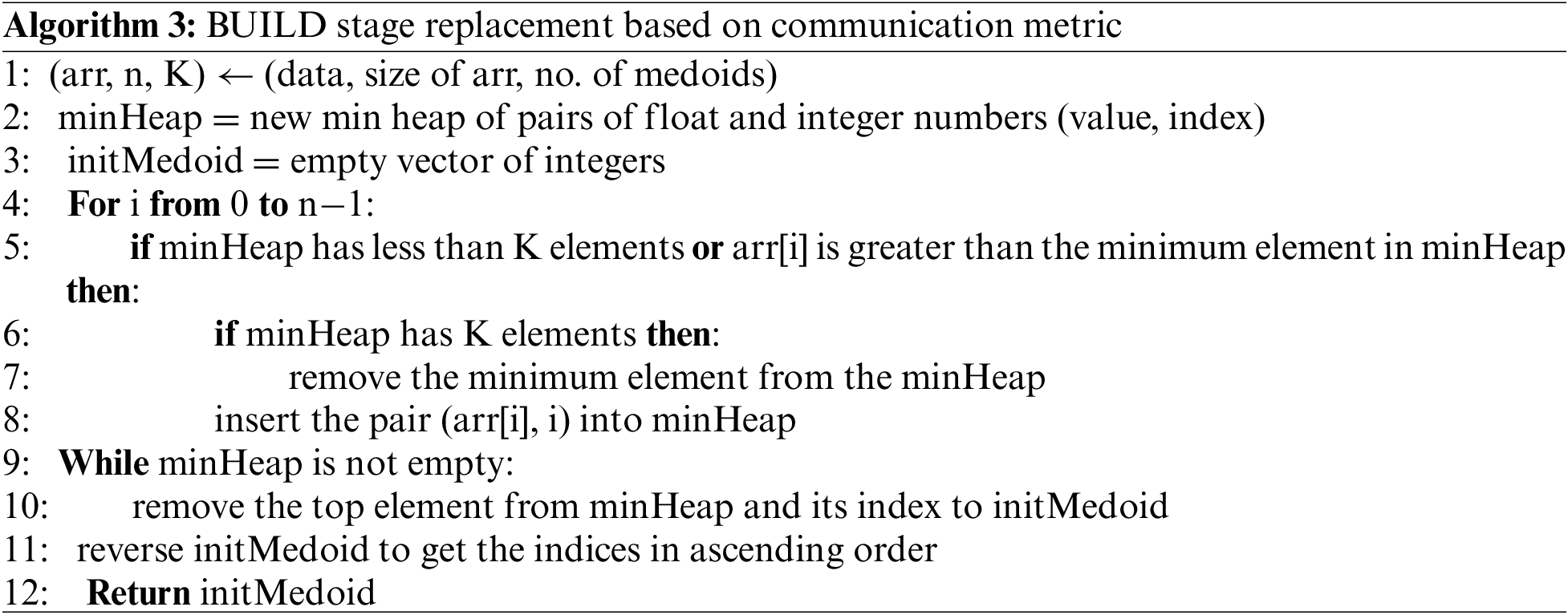
The pseudo-code in Algorithm 3 uses a min-heap data structure of pairs of integers to store the elements (VehRxdBm or AvgLET) and their indices (vehicle ID). The function iterates through the input array arr and adds each element and its index as a pair to the min heap if the heap has less than K elements or the element is greater than the minimum element in the heap. Once the heap has K elements, the minimum element is removed before adding a new element. After adding all the elements to the heap, the top K elements are extracted from the heap by removing the top element K times and adding its index to the initMedoid vector. The initMedoid vector is reversed to get the indices in ascending order since the heap stores the elements in ascending order by value. Finally, the function returns the initMedoid vector containing the indices of the largest K elements in the input array.

The time complexity of Algorithm 3 is O(n log K), where n is the size of the input array, and K is the number of largest values required. In the worst case, insertion of each element into the min heap takes O(log K) time since it might need to bubble up the element to maintain the heap property. The insertion is done n times for each element in the input array, so the total time for building the min heap is O(n log K). Extracting the largest K elements from the min heap also takes O(K log K) time in the worst case since it is required to extract the top element and possibly bubble down a new root element to maintain the heap property after each extraction. The extraction is done K times for the largest K elements, so the total time for extracting the largest K elements is O(K log K). Therefore, if K is much smaller than n, the min heap approach can be significantly faster than sorting the entire array and extracting the largest K elements. However, if K is close to n, the sorting method may be more rapid since the cost of sorting the array will be similar to that of extracting the largest K elements using a min-heap.

3.4 The Evaluation Process

The evaluation process of estimating the K number and the clustering algorithms will be mentioned in this section. In terms of estimating the K number, the output of Scott’s formula for the inputs mentioned in Section 3.3 is evaluated against the estimated number of clusters by the Affinity propagation algorithm when the Euclidean distance and LET are used. Because the Scott’s formula (1) assumes the input data is normally distributed, the Shapiro-Wilk normality test is implemented on the formula’s inputs to evaluate its validity. Moreover, Medoid-Silhouette (MS) width analysis is implemented on the selected K to evaluate its fitness. Also, the MS score is used to construct a curve similar to the elbow curve to quantify the clustering algorithms. The average and mid-range values are calculated for a range of K to evaluate the MS curves. The range of K for this calculation has a lower bound of 10% of the number of vehicles and half of the total number of vehicles as the upper bound. If more than half of the vehicles became CHs, clusters might only contain one vehicle, which is pointless. Moreover, having less than 10% of the vehicles selected as CHs is impractical.

The Medoid-Sillhouette method is selected because not all vehicles in the range of the RSU are in the communication range of each other. Therefore, the MS score could indicate how close a vehicle is to its CH compared to the other CHs. Furthermore, ditching the BUILD stage in favor of the VehRxdBm or AvgLET base initial medoids selection will be evaluated based on the number of iterations and swaps implemented by the SWAP stage alone vs. the original FastPAM. This modified version of the FastPAM algorithm will be called the Lightweight FastPAM Vehicular Clustering algorithm (LFPVC) and referred to in this work as LFPVC(VehRxdBm) and LFPVC(AvgLET) based on the metric replacing the BUILD stage. Finally, the chosen maps will evaluate the suggested methods against various road layouts and traffic flow. Fig. 2 shows the process followed by this work to gather the data from the simulations and implement the clustering algorithms.

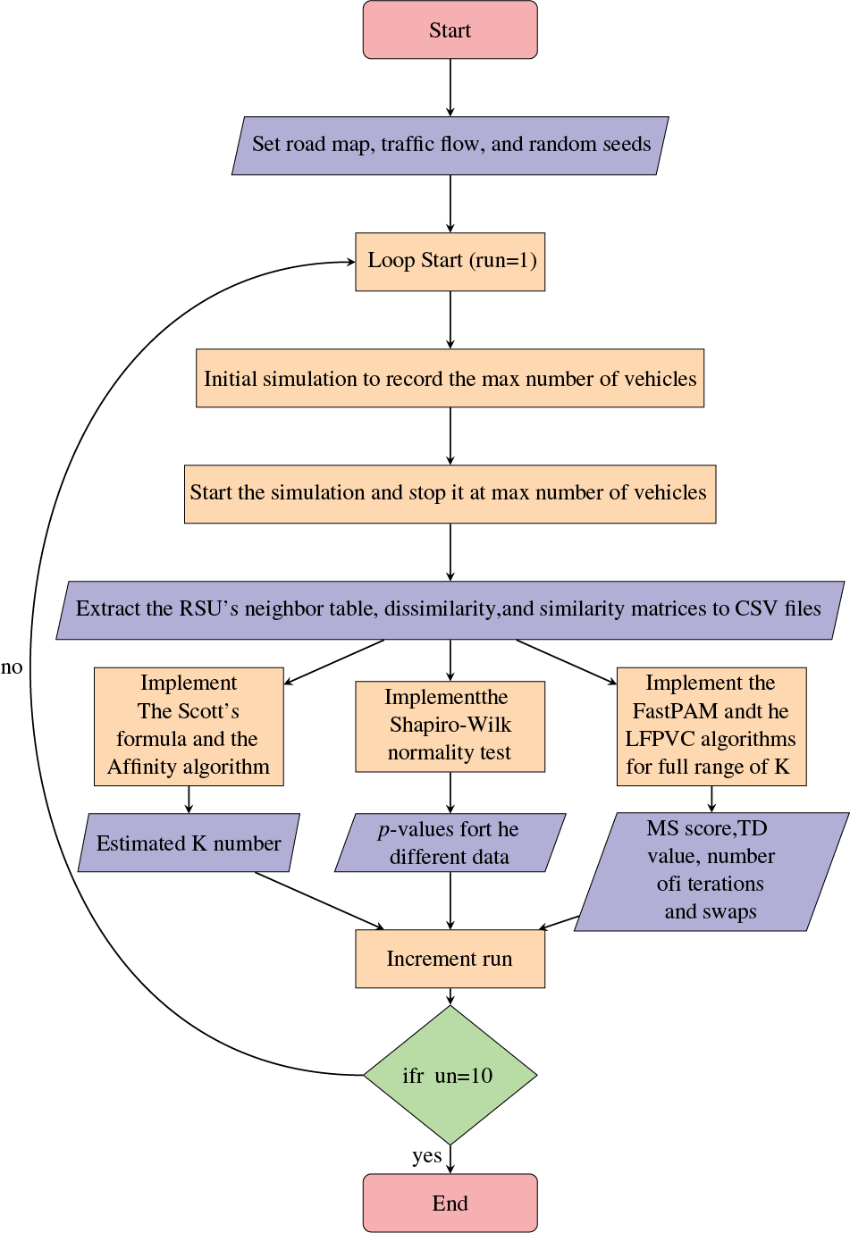
Figure 2: The process of the VANET simulation, clustering and data gathering

4  Results and Discussion

The vehicular network model was simulated using OMNET++ 5.6.2 and Veins 5.2, while the vehicle mobility model and road network were created with SUMO 1.8 on a computer running Ubuntu 20.04 operating system. Table 2 shows two traffic flow scenarios for each of the three road maps. The neighbor table of RSU is recorded at the end of the simulation time of the six scenarios. The RSU is deployed in the middle of the junctions and the highway maps (Fig. 1) to gather the BSMs sent by the vehicles and build the neighbor table, which is exported as a CSV file (Fig. 2). This work implements the FastPAM algorithm on the collected neighbor tables using the “kmedoids” Python library [34]. The kmedoids library allows the FastPAM’s SWAP stage to be implemented separately by feeding the indexes of the initial medoids. Therefore, the default BUILD stage can be replaced with the use of vehicle communication metrics to select the K initial medoids (Algorithm 3). The baseline for estimating the K number is obtained by implementing the Affinity propagation algorithm using the “sklearn” Python library on the recorded data. Both libraries allow the mentioned algorithms to accept dissimilarity matrix. Therefore, the LET matrix is generated and prepared as a negative similarity matrix with the infinity values replaced with the maximum non-infinity LET value. The figures below illustrate the results for the six simulation scenarios; Highway with High Flow (HW-HF), Highway with Low Flow (HW-LF), Traffic light with High Flow (TL-HF), Traffic light with Low Flow (TL-LF), Roundabout with High Flow (RA-HF), and Roundabout with Low Flow (RA-LF). Each of the six simulation scenarios is executed ten times by feeding the SUMO random seeds to obtain different mobility patterns.

The bar chart in Fig. 3 shows the rounded average of the simulation runs for the estimated K number by the Scott’s formula for different inputs and the Affinity algorithm when LET (Affinity(LET)) and Euclidean distance (Affinity(Dis)) are used. The VehRxdBm input for the Scott’s formula is the only metric registered from the vehicle’s viewpoint. Thus it can give a reasonable estimate of the number of clusters. Individually, the X and Y coordinates cannot give a complete estimate of the number of clusters because the formula will count for the frequency of vehicles sharing the same X or Y coordinate. This invalidity is clear in the results of the TL scenarios. The RSU in the TL scenarios covers more of the road in the Y direction than in the HW and RA scenarios. Using the RSU as a reference for the Dis2RSU and RSURxdBm input cannot give optimal estimation because not all vehicles in the RSU communication range are within range of each other. The same goes for the AvgDis input because the data is gathered from the RSU.

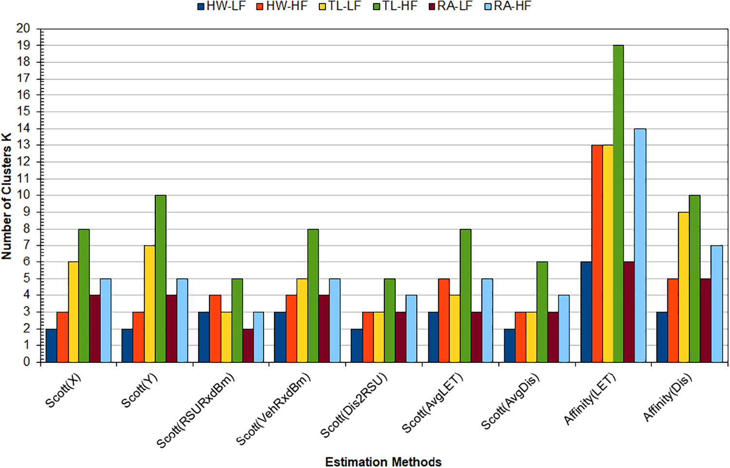
Figure 3: The estimated K number by Scott’s formula and the Affinity algorithm

It is still a valid comparison between the inputs above and those of the Affinity algorithm (Dis and LET), as they are based on the RSU neighbor table. However, the Scott’s formula results in Fig. 3 did not clearly match the estimated K number by the Affinity algorithm. The estimated K numbers by Affinity (LET) exceeded all other cases. However, the K numbers estimated for the HW-HF and HL-LF simulation scenarios by Scott’s formula with VehRxdBm and AvgLET slightly match those by Affinity (Dis). These results might indicate that Scott’s formula is not optimal for estimating the K number in complex road layouts. Scott’s formula (1) assumes the data is normally distributed. Thus, the data of the ten simulation runs were tested using the Shapiro-Wilk normality test. Table 3 shows the percentage of normally distributed data from the ten runs for the six simulated scenarios.

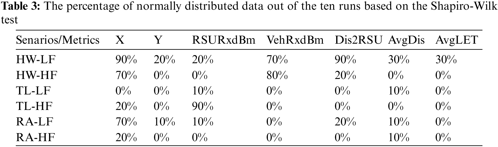
A communication-based metric such as VehRxdBm or AvgLET can be a valid input for the formula rather than a geometry-based metric such as the coordinates or distance to RSU. For the HW scenarios, the X coordinate and the VehRxdBm data are mainly normally distributed (Table 3). However, the trend did not continue for the VehRxdBm in the TL and RA scenarios. Even though the Scott(AvgLET) result matched the Affinity(Dis) estimation of the K number for the HW scenarios (Fig. 3), the AvgLET data is not normally distributed for all the scenarios (Table 3). Moreover, the data were represented in quantiles (Q-Q) plots (not included in this work). The Q-Q plots of the AvgLET data showed a trend of horizontal line of points across the plots for all scenarios. The horizontal line trend also appeared on the Q-Q plots of the VehRxdBm data for the RA and TL scenarios. This trend indicates that the AvgLET and VehRxdBm follow a different distribution in the mentioned scenario. Therefore, histograms of ten bins were drawn for the AvgLET and VehRxdBm data (not included in this work), showing the AvgLET date positively skewed with a long tell to the right side of the plots. The VehRxdBm data were negatively skewed with long tell to the left side of the histogram plots. Logarithmic and exponential functions were implemented to the AvgLET and VehRxdBm data, respectively, to reduce the skewness of the data. However, it did not help to transform the AvgLET and VehRxdBm data to normal distribution according to the Shapiro-Wilk test.

Histogram bin number formulas such as the Freedman and Diaconis formula, which rely on the IQR of the data, do not assume the distribution of the data. However, reference [7] concluded that the time complexity of IQR is higher than computing the standard deviation of the data because the IQR requires sorting the data. Moreover, the IQR relies on the position of the data point rather than its value. Therefore, the Freedman and Diaconis formula is not optimal for estimating the K number for a VN clustering algorithm. The results of Fig. 3 and Table 3 might indicate that the Scott’s formula is not optimal for estimating the K number in complex road layouts. However, a communication-based metric such as VehRxdBm can still be a valid input for the formula for a specific scenario rather than the geometry-based metrics.

The affinity algorithm uses a similarity metric to establish the correlation among the data points and estimate the number of clusters. Moreover, the damping factor and the preference of the affinity algorithm affect its estimation of the number of clusters. However, increasing the damping factor to more than 0.5 did not change the estimated K number when the LET is used as the clustering metric. The preference was set by default to the median of the similarity matrix. The average median values were 5, 46, and 18 for the HW, TL, and RA scenarios, respectively. These preference values are reasonable for the scenarios because they represent an estimate for the connection period in seconds between two vehicles. Increasing the preference will increase the number of clusters, and decreasing the preference will lead to including vehicles with non-optimal connection time in the cluster.

To further evaluate the fitness of the estimated K numbers by the methods above, a width analysis for the Medoid-Silhouette (MS) score is done on the highway scenarios. The data from the simulation runs with the largest number of vehicles recorded at the end of the simulation are used for this analysis. The highway scenarios were selected because the Scott (VehRxdBm) gave the closest K number estimate to the one by the Affinity (Dis). Moreover, the VehRxdBm matched the data distribution requirement of Scott’s formula. For the HW-HF scenario, the estimated K numbers were 4, 13, and 5 for the Scott (VehRxdBm), Affinity (LET), and Affinity (Dis), respectively. And for the HW-LF scenario, the estimated K numbers were 3, 6, and 3 for the Scott (VehRxdBm), Affinity (LET), and Affinity (Dis), respectively. Fig. 4 illustrates the MS width for the clusters based on the estimated K numbers from the data of simulation runs number seven and three for the HW-HF and HW-LF scenarios, respectively. The assignment of the clusters is based on the FastPAM algorithm’s results with the LET as the clustering metric. It must be noted that the MS score for the medoid is one. Therefore, each cluster in Fig. 4 must have at least one unit value bar.

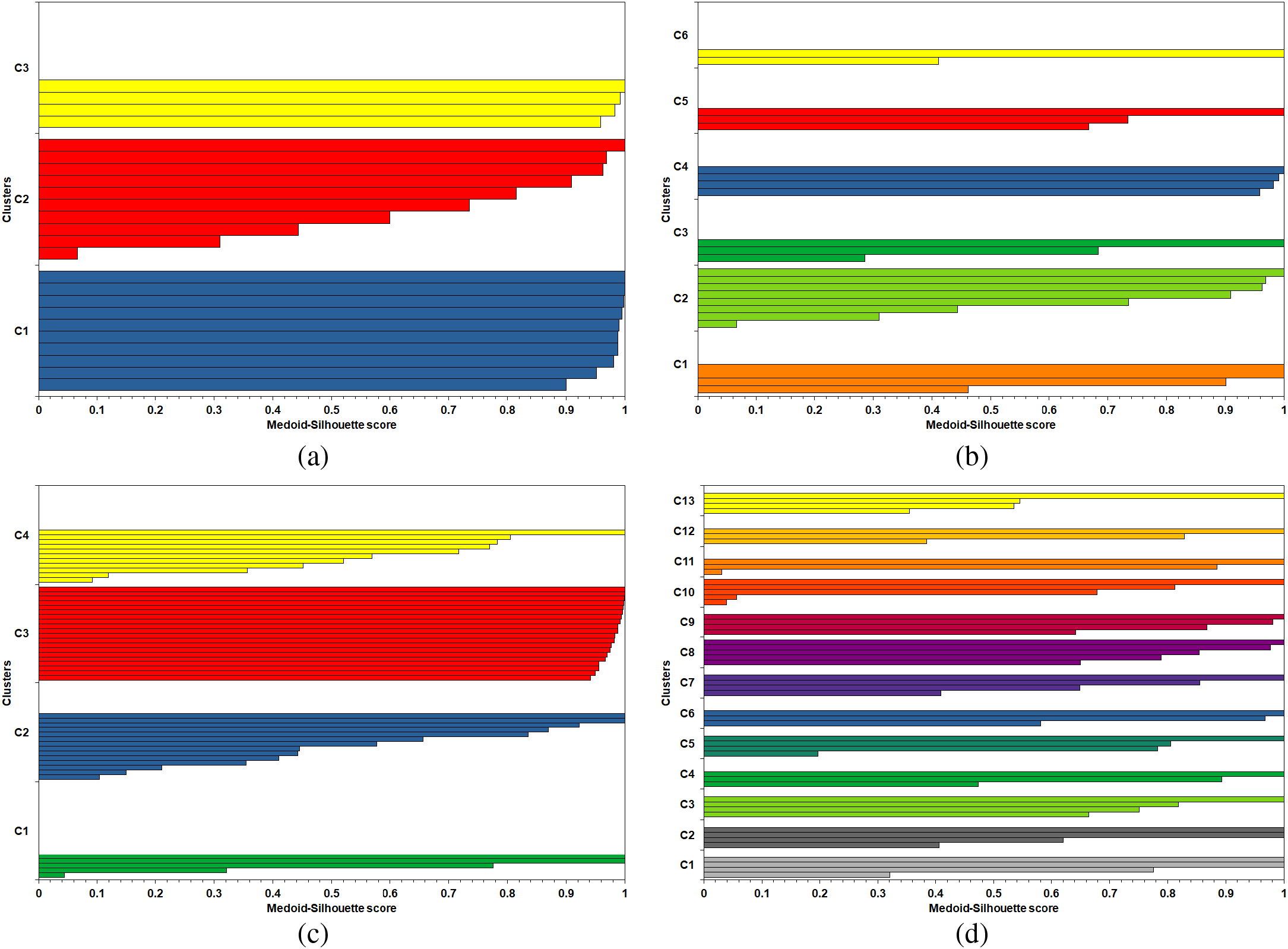
Figure 4: The Medoid-Silhouette width for the Highway road map: (a) LF scenario and K = 3, (b) LF scenario and K = 6, (c) HF scenario and K = 4, (d) HF scenario and K = 13

For the HW-LF, Fig. 4a shows uniform MS widths among the clusters, while Fig. 4b contains a cluster with only one member besides the medoid. Moreover, without considering the MS score for the medoids, some of the cluster plots in Fig. 4b present below the average MS score (0.769) of the simulation scenario. In Fig. 4a, all the cluster plots pass the scenario’s average MS score (0.856). For these reasons, Scott(VehRxdBm)’s K estimation of three is optimal for the HW-LF scenario. Regarding the HW-HF scenario, the cluster plots in Fig. 4c have fluctuations in size and presence above their MS average (0.738). Moreover, when K equals 13, the plots’ width is more consistent among the cluster (Fig. 4d). However, without considering the medoids of the clusters, cluster (C13) in Fig. 4d did not pass the scenario’s MS average (0.737). And clusters (C10 and C11) in Fig. 4d contain members with MS scores below 0.1, which means they do not fit well in their clusters.

The MS curves from the FastPAM algorithm of the runs with the largest number of vehicles recorded at the end of the simulation are shown in Fig. 5. The average of the MS curves for the ten runs is shown in Fig. 6. The MS curves in Fig. 6 are clipped to the lowest number of vehicles, as not all runs have the same number. The noticeable pattern in these curves is the flattening after a certain number of K.

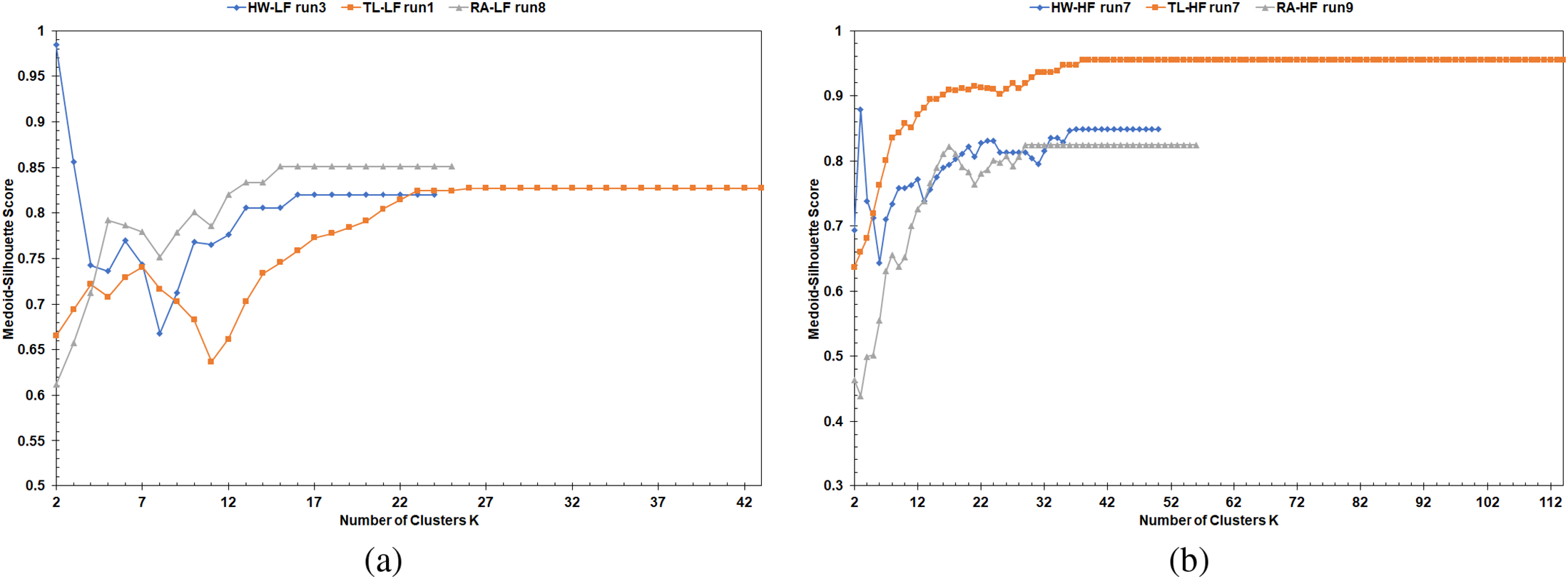
Figure 5: MS curves from FastPAM: (a) LF scenarios, (b) HF scenarios

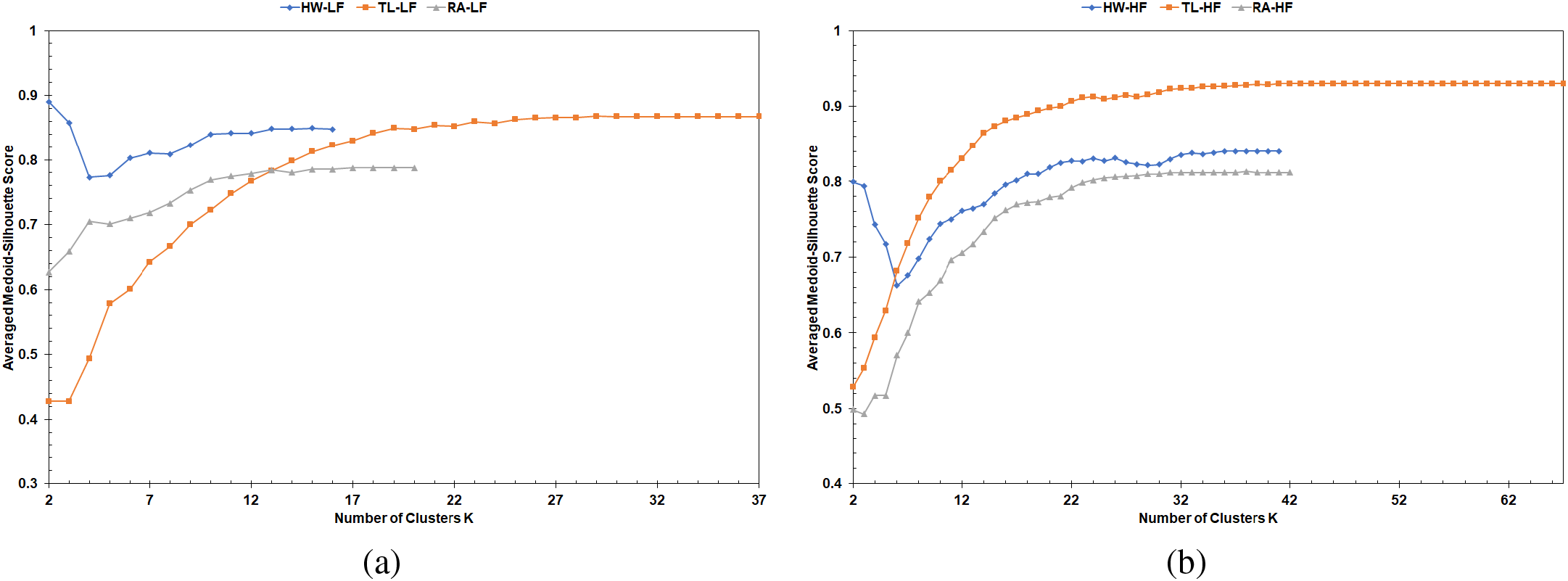
Figure 6: Average MS curves from FastPAM: (a) LF scenarios, (b) HF scenarios

The BUILD stage (Algorithm 1) iterates for the required K medoids. Still, it only adds the candidate medoid, reducing the ΔTD to the final list of initial medoids. The SWAP stage takes the initial medoids list and tries to optimize it by swapping the selected medoids with the non-selected ones that can reduce the ΔTD. The LET metric allows multiple vehicles to have maximum similarity value with other vehicles besides itself. This redundancy restricts the K number because considering these vehicles with large LET values as medoids will not change the ΔTD. Thus when LET is used, the BUILD stage clips the required K medoids to those fitting the total deviation reduction condition (Algorithm 1 line 15). Moreover, the clipping effect occurs because not all vehicles are in communication range of each other (zero LET value), and increasing the K number does not guarantee enough valid medoids. Also, the MS curves in Fig. 5 showed fuzziness when K is low, but the averaged MS curves in Fig. 6 present a logarithmic-like curve before it reaches the flattened section.

The MS curves from implementing the FastPAM algorithm with Euclidean distance for the same simulation runs are shown in Figs. 7 and 8. The lack of the flattened section at the end of these curves is because the Euclidean distance is computable for all vehicles, and any two vehicles can not share the exact location (i.e., zero dissimilarity value between them). Therefore, the lack of this pattern cements the superiority of LET over the Euclidean distance as a clustering metric for the vehicular network. The MS curves from implementing LFPVC(VehRxdBm) are shown in Figs. 9 and 10. Moreover, Figs. 11 and 12 illustrate the results of implementing LFPVC(AvgLET). The effect of not using the original BUILD stage is shown in Figs. 9 and 11, as the MS curves did not show the same flat-end pattern as in Fig. 5. However, the only pattern that can be noticed from the figures below is the steep incline after the fuzzy beginning of the curves, just like the MS curves of the FasterPAM with Euclidean distance.

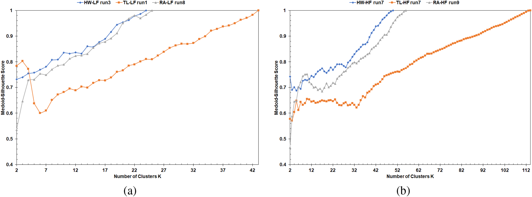
Figure 7: MS curves from FastPAM using Euclidean distance: (a) LF scenarios, (b) HF scenarios

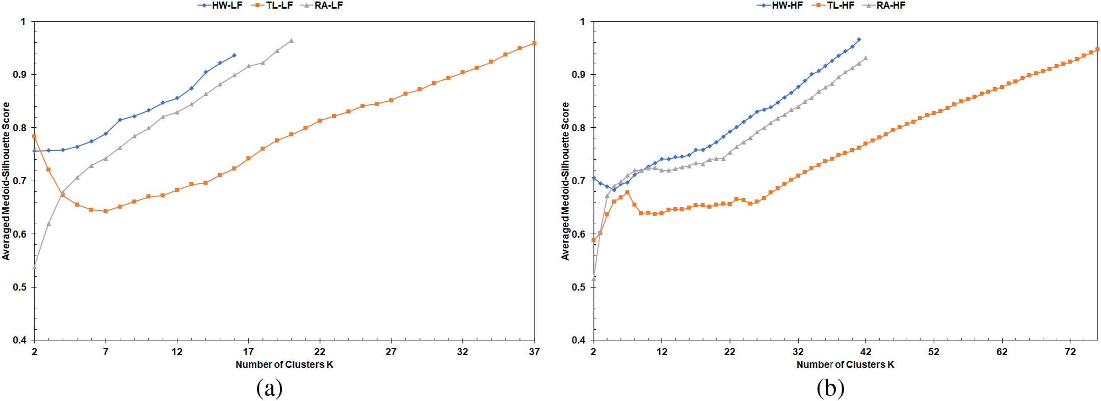
Figure 8: Average MS curves from FastPAM using Euclidean distance: (a) LF scenarios, (b) HF scenarios

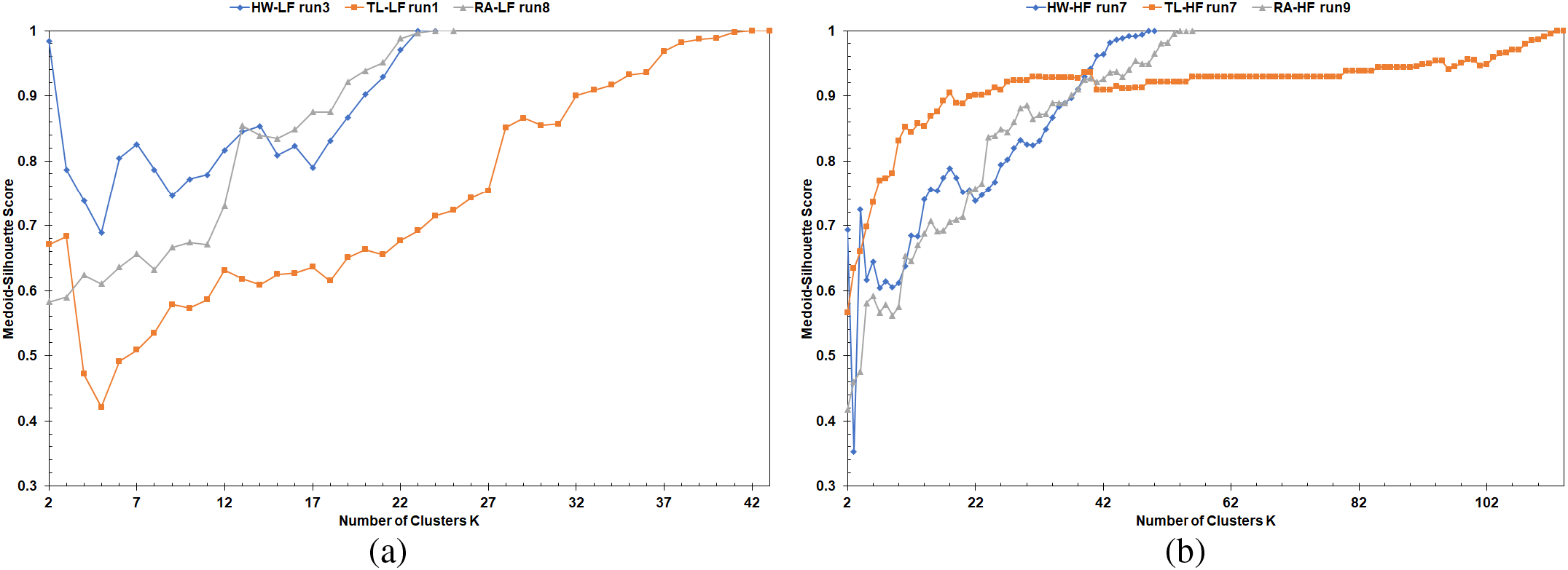
Figure 9: MS curves from LFPVC(VehRxdBm): (a) LF scenarios, (b) HF scenarios

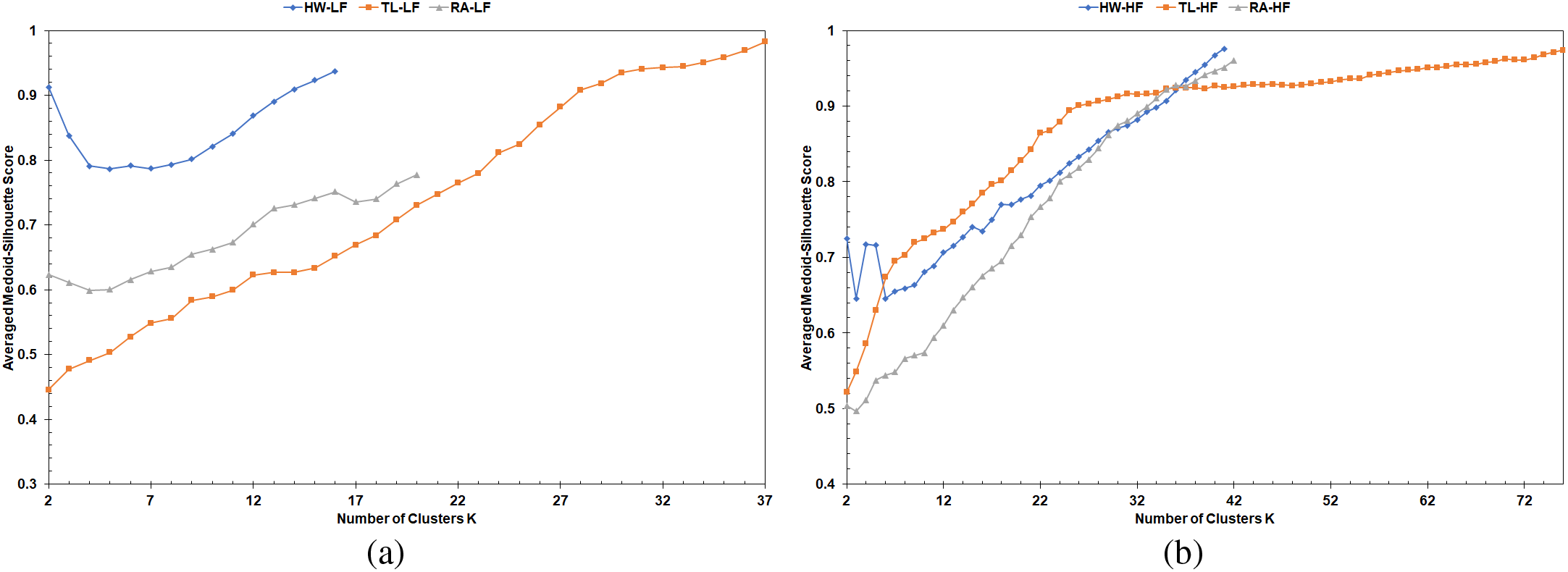
Figure 10: Average MS curves from LFPVC(VehRxdBm): (a) LF scenarios, (b) HF scenarios

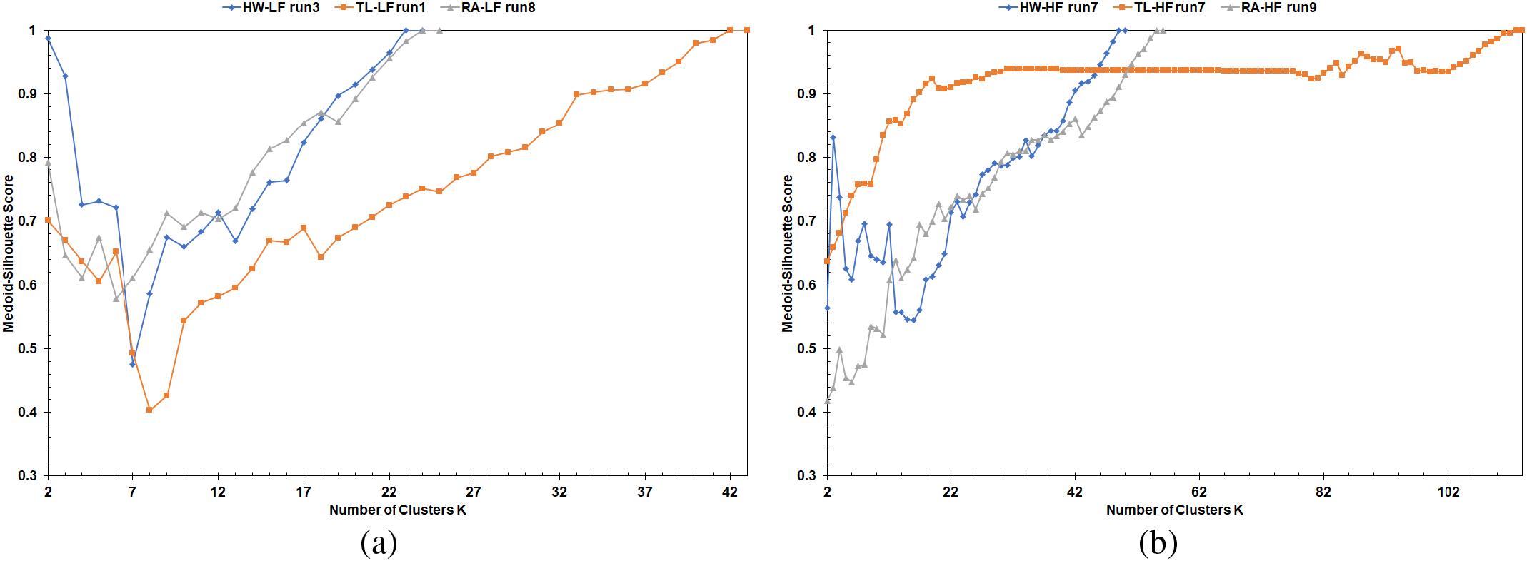
Figure 11: MS curves from LFPVC(AvgLET): (a) LF scenarios, (b) HF scenarios

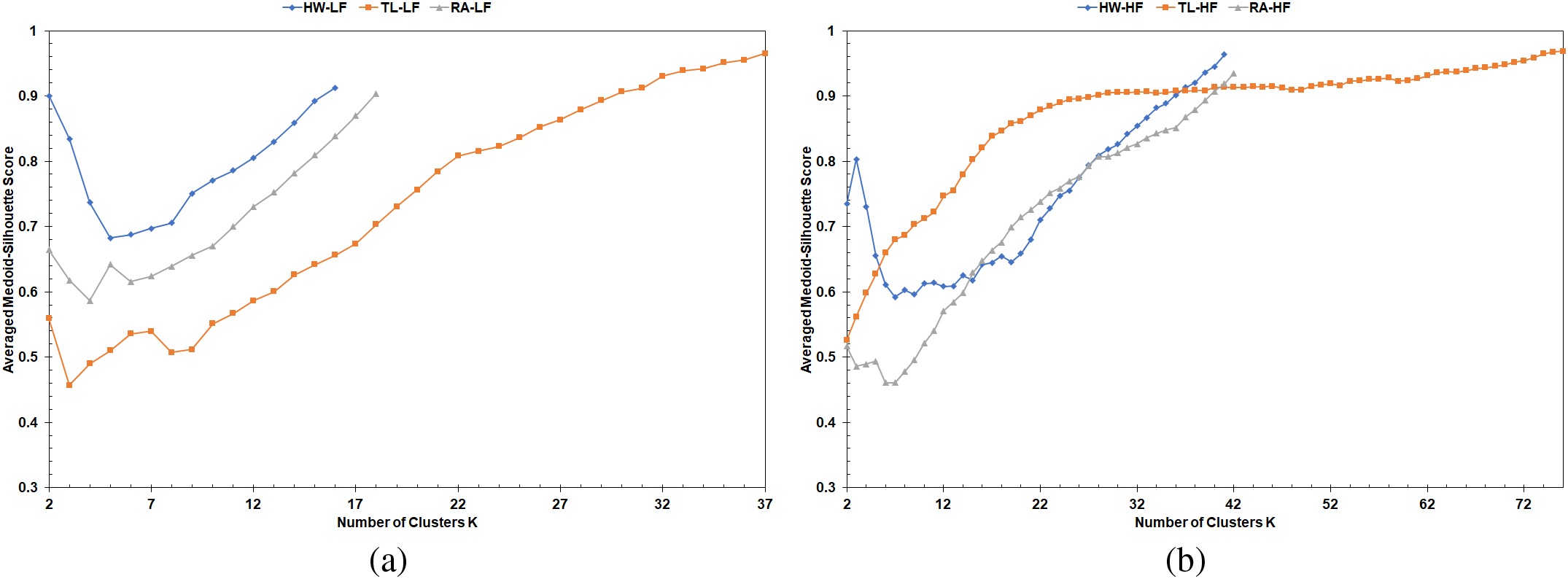
Figure 12: Average MS curves from LFPVC(AvgLET): (a) LF scenarios, (b) HF scenarios

The MS curves of the average runs in Figs. 6, 10, and 12 did not include a pattern that helps quantify picking the initial medoids based on the VehRxdBm or the AvgLET metric. Therefore, the mid-range and average of the MS curves based on the effective K range, explained in Section 3.4, were computed for the simulation scenarios. Fig. 13 illustrates the mid-range values of the MS curves for the runs with the largest number of vehicles and the average of the ten runs. The average values of the MS curves for the runs with the largest number of vehicles and the average of the ten runs are demonstrated in the bar charts of Fig. 14. The mid-range values from the bar charts in Fig. 13 were not decisive on the FastPAM algorithm yielding higher mid-range values when modified with either the VehAvgdBm or the AvgLET metrics.

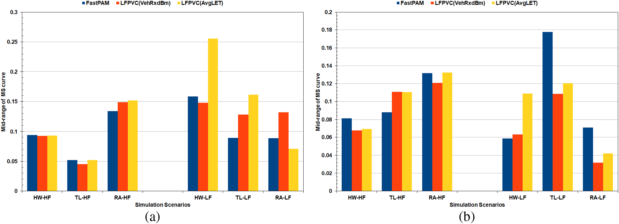
Figure 13: Mid-range of the MS curves: (a) Runs of the largest number of vehicles, (b) Average of the runs

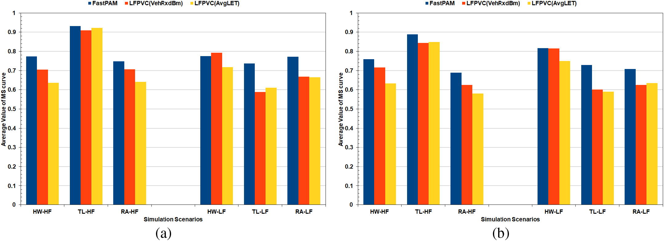
Figure 14: Average of the MS curves: (a) Runs of the largest number of vehicles, (b) Average of the runs

However, the average values for the MS curves of the FastPAM were, in most cases, slightly higher than those of the modified algorithms (Fig. 14). The mid-range and average values of the MS curves could not prove that ditching the BUILD stage in favor of the VehAvgdBm and AvgLET is profitable. The suggested methods (LFPVC(VehRxdBm) and LFPVC(AvgLET)) could not match the greedy process of the original BUILD stage. However, the effective K range on which the bar charts of Fig. 13 and 14 are based falls mainly in the fuzzy sections of the MS curves.

The MS curves could not give an insight into to which degree the suggested replacements of the original BUILD stage are profitable or feasible. Therefore, the TD values for the average runs of the highway scenarios are plotted against K in Fig. 15. The FastPAM, when implemented with negative LET, returns a negative TD. Therefore, the average TD’s absolute values are shown in Fig. 15, which illustrates inverted Elbow curves. Unlike the traditional Elbow curve, the TD value in Fig. 15 increases as the number of K increases. In both LF and HF scenarios, the FastPAM recorded higher averaged TD values before the flattening pattern arose than the LFPVC(VehRxdBm) and LFPVC(AvgLET). However, the averaged TD values of the LFPVC(VehRxdBm) are relatively closer to the optimal ones of the FastPAM (Fig. 15).

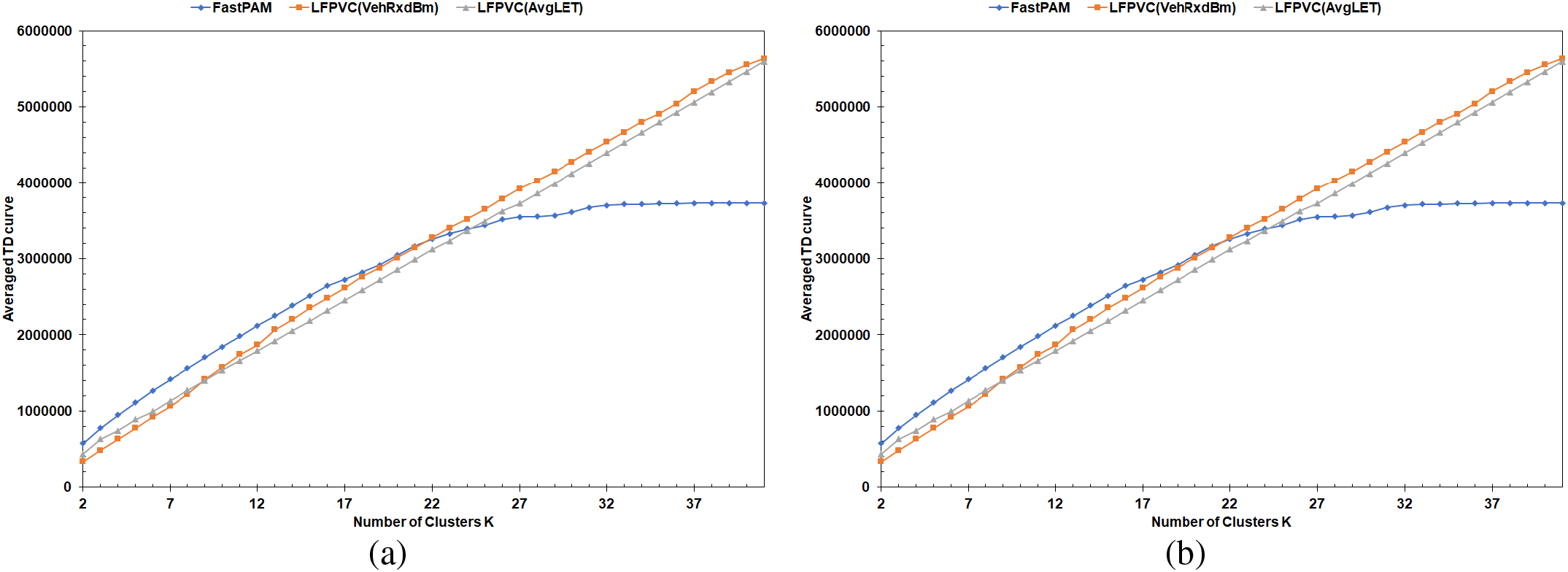
Figure 15: TD curves of the average runs: (a) HW-LF, (b) HW-HF

Finally, to evaluate the performance of the FastPAM, LFPVC(VehRxdBm), and LFPVC(AvgLET) algorithms, the average number of iterations and swaps implemented by the SWAP stage was recorded and illustrated in Fig. 16. Moreover, the average number of iterations and swaps of the original FastPAM algorithm when implemented with the Euclidean distance is shown in Fig. 16 and annotated as FastPAM-DIS. The bar chart of Fig. 16 is based on the simulation runs with the largest number of vehicles.

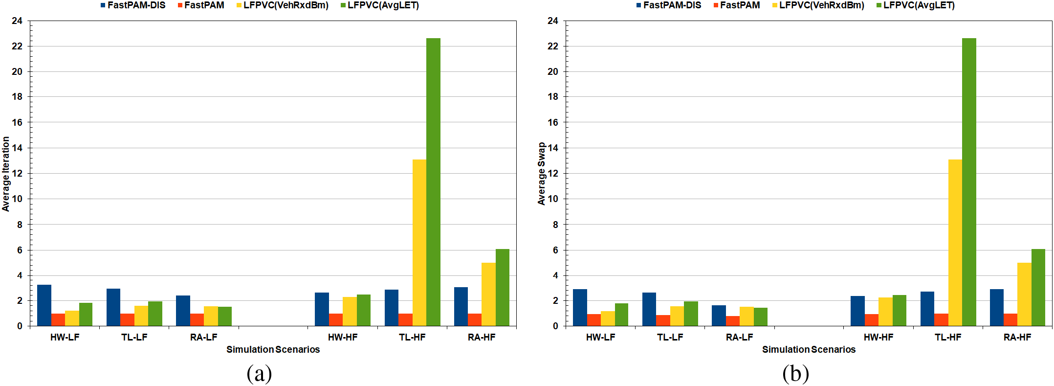
Figure 16: The average number of iterations and swaps implemented by the SWAP stage: (a) Average iteration, (b) Average swap

Using the LET metric is optimal for vehicle clustering, as the original algorithm with LET (FastPAM) required one iteration/swap on average to converge (Fig. 16). In contrast, FastPAM-DIS required 2.8 iterations and 2.5 swaps on average for all scenarios. The LFPVC(VehRxdBm) and LFPVC(AvgLET) required 4 and 6 iterations/swaps on average for all scenarios, respectively. However, LFPVC(VehRxdBm) recorded 1.4 iterations/swaps on average, and LFPVC(AvgLET) required an average of 1.7 iterations/swaps to converge for all the LF scenarios. The high traffic flow heavily affected the performance of the modified algorithms. The average iterations and swaps from the TL-HF and RA-HF scenarios for the LFPVC algorithms were around twenty times higher than those from the HW-HF scenarios (Fig. 16). This extreme increase in the average number of iterations and swaps proves that selecting the initial medoids based on the VehRxdBm and AvgLET metrics is not optimal when the road layout is complex.

5  Conclusions

This work examined the suggested method of using the Scott’s histogram formula to estimate the number of clusters and using the LET metric for vehicular clustering. Moreover, it evaluated the replacement of the greedy process, selecting the initial medoids for the FastPAM algorithm by selecting the initial K medoids based on vehicle communication metrics. Furthermore, negative values of the LET metric and the maximum LET value instead of infinity LET values in the similarity matrix are considered to avoid modifying the FastPAM algorithm. The number of clusters estimated by the Affinity Propagation algorithm was the baseline for estimating the K number. The Affinity algorithm is an approximation method to maximize the similarity. Thus, an exact match between the results of the Affinity algorithm and Scott’s formula was not expected. This work suggested presenting the Medoid-Silhouette score as a curve for the range of K to benchmark the algorithms, LFPVC(VehRxdBm), and LFPVC(AvgLET) against the FastPAM algorithm.

The Scott’s formula failed to match the K number estimation of the Affinity propagation algorithm for most of the formula’s inputs. However, the Scott’s formula and the Affinity algorithm showed a correlation in highway simulations with VehRxdBm as input and Euclidean distance as clustering metric. The matching in results is backed up with the normal distribution of the VehRxdBm data in the highway scenarios and further clarified with the width silhouette analysis. Therefore, Scott’s formula method works better with the VehRxdBm metric and simple road layout because the formula assumes the data to be normally distributed. However, The VehRxdBm and AvgLET data showed skewed distributions in the complex road layout scenarios. The high time complexity deters from using histogram bin number formulas that do not rely on the distribution of the data. Plotting the average MS score for the range of K did not provide a clear pattern to quantify the LFPVC(VehRxdBm) and LFPVC(AvgLET). However, the flattening at the end of the MS curves for the original algorithm proved the efficiency of using LET for vehicular clustering. Also, the original BUILD stage clipped the number of K to the maximum possible number of medoids as not all vehicles have connections to each other or can contribute to the reduction of ΔTD. The LFPVC(VehRxdBm) showed feasibility for clustering under the condition of a simple road layout. This conclusion is based on the slight matching with the TD curves of the FastPAM algorithm, and the average number of iterations/swaps was lower than that of the LFPVC(AvgLET). Moreover, a related work validated the LET metric for highway traffic scenarios.

Finally, setting a baseline for vehicular clustering is challenging as the data are not explicitly labeled. Even though the Affinity Propagation algorithm simulates the exchange of messages among the vehicles to compute the fitness of the CH, it is also considered an approximation method to maximize the similarity. Moreover, the preference value in the LET similarity matrix beside its diagonal can explain the high K number estimation by the Affinity algorithm. Therefore, the K estimation by Scott’s formula is fit as the formula’s input because the input must satisfy the formula’s distribution requirement and present adequate CH validity for the vehicles. Besides the algorithm, clustering in the VN environment relies on exchanging control messages to form and maintain the clusters, which is not the focus of this work. Furthermore, the computation of the average received power by the vehicle (VehRxdBm) can be improved by including the average LET value. The future work will consider a clustering scheme that uses an adequate input for the Scott’s formula and evaluate the output based on cluster lifetime and communication delay.

Acknowledgement: The authors would like to thank Professor Erich Schubert of TU Dortmund University for his help in understanding the working principles of the PAM and FastPAM algorithms.

Funding Statement: The authors received no specific funding for this study.

Author Contributions: The authors confirm contribution to the paper as follows: Conceptualization, Fady Samann; Formal analysis, Fady Samann; Investigation, Fady Samann; Methodology, Fady Samann; Resources, Shavan Askar; Software, Fady Samann; Supervision, Shavan Askar; Writing—original draft, Fady Samann; Writing—review and editing, Shavan Askar. All authors reviewed the results and approved the final version of the manuscript.

Availability of Data and Materials: The recorded neighbor tables and the generated similarity/dissimilarity matrices are publicly available at https://github.com/FadySamann/RSUrecordedData.

Conflicts of Interest: The authors declare that they have no conflicts of interest to report regarding the present study.

References

1. Ayyub, M., Oracevic, A., Hussain, R., Khan, A. A., Zhang, Z. (2022). A comprehensive survey on clustering in vehicular networks: Current solutions and future challenges. Ad Hoc Networks, 124, 102729. [Google Scholar]

2. Cooper, C., Franklin, D., Ros, M., Safaei, F., Abolhasan, M. (2017). A comparative survey of VANET clustering techniques. IEEE Communications Surveys & Tutorials, 19(1), 657–681. [Google Scholar]

3. Samann, F. E. F., Abdulazeez, A. M., Askar, S. (2021). Fog computing based on machine learning: A review. International Journal of Interactive Mobile Technologies (iJIM), 15(12), 21–46. [Google Scholar]

4. Schubert, E., Rousseeuw, P. J. (2019). Faster k-Medoids clustering: Improving the PAM, CLARA, and CLARANS algorithms. in: Lecture notes in computer science (including subseries lecture notes in artificial intelligence and lecture notes in bioinformatics), vol. 11807, pp. 171–187. Cham: Springer. [Google Scholar]

5. Schubert, E., Rousseeuw, P. J. (2020). Fast and eager k-Medoids clustering: O(k) runtime improvement of the PAM, CLARA, and CLARANS algorithms. Information Systems, 101, 101804. [Google Scholar]

6. Celebi, M. E. (2015). Partitional clustering algorithms. Cham: Springer International Publishing. [Google Scholar]

7. Samann, F. E. F., Askar, S. (2022). Estimating the optimal cluster number for vehicular network using Scott’s formula. 2022 4th International Conference on Advanced Science and Engineering (ICOASE), Zakho, Iraq, IEEE. [Google Scholar]

8. Su, W., Lee, S. J., Gerla, M. (2001). Mobility prediction and routing inad hoc wireless networks. International Journal of Network Management, 11(1), 3–30. [Google Scholar]

9. Cardote, A., Sargento, S., Steenkiste, P. (2010). On the connection availability between relay nodes in a VANET. 2010 IEEE Globecom Workshops, Miami, FL, USA, IEEE. [Google Scholar]

10. Scott, D. W. (2010). Scott’s rule. Wiley Interdisciplinary Reviews: Computational Statistics, 2(4), 497–502. [Google Scholar]

11. Athab, H., Al-Jameel, E., Abbas, M., Al-Jumaili, H. (2016). Analysis of traffic stream characteristics using loop detector data. Jordan Journal of Civil Engineering, 10(4), 403–416. [Google Scholar]

12. National Research Council (U.S.Transportation Research Board (2000). Highway capacity manual. Washington DC, USA: Transportation Research Board, National Research Council. [Google Scholar]

13. National Research Council (U.S.) (2016). Highway capacity manual: A guide for multimodal mobility analysis. Washington DC, USA: Transportation Research Board, National Research Council. [Google Scholar]

14. Katiyar, A., Singh, D., Yadav, R. S. (2020). State-of-the-art approach to clustering protocols in VANET: A survey. Wireless Networks, 26(7), 5307–5336. [Google Scholar]

15. Mirkin, B. (2011). Choosing the number of clusters. WIREs Data Mining and Knowledge Discovery, 1(3), 252–260. [Google Scholar]

16. Antunes, M., Gomes, D., Aguiar, R. L. (2018). Knee/elbow estimation based on first derivative threshold. 2018 IEEE Fourth International Conference on Big Data Computing Service and Applications (BigDataService), Bamberg, Germany, IEEE. [Google Scholar]

17. Satopaa, V., Albrecht, J., Irwin, D., Raghavan, B. (2011). Finding a “Kneedle” in a haystack: Detecting knee points in system behavior. 2011 31st International Conference on Distributed Computing Systems Workshops, Minneapolis, MN, USA, IEEE. [Google Scholar]

18. Shi, C., Wei, B., Wei, S., Wang, W., Liu, H. et al. (2021). A quantitative discriminant method of elbow point for the optimal number of clusters in clustering algorithm. EURASIP Journal on Wireless Communications and Networking, 2021(1), 31. [Google Scholar]

19. Lengyel, A., Botta-Dukát, Z. (2019). Silhouette width using generalized mean-A flexible method for assessing clustering efficiency. Ecology and Evolution, 9(23), 13231–13243. [Google Scholar] [PubMed]

20. Saputra, D. M., Saputra, D., Oswari, L. D. (2020). Effect of distance metrics in determining K-value in K-means clustering using Elbow and silhouette method. Proceedings of the Sriwijaya International Conference on Information Technology and Its Applications (SICONIAN 2019), vol. 172. Paris, France, Atlantis Press. [Google Scholar]

21. Lenssen, L., Schubert, E. (2022). Clustering by direct optimization of the medoid silhouette. In: Similarity search and applications (SISAP 2022), vol. 13590. Cham: Springer International Publishing. [Google Scholar]

22. Tibshirani, R., Walther, G., Hastie, T. (2001). Estimating the number of clusters in a data set via the gap statistic. Journal of the Royal Statistical Society: Series B (Statistical Methodology), 63(2), 411–423. [Google Scholar]

23. Frey, B. J., Dueck, D. (2007). Clustering by passing messages between data points. Science, 315(5814), 972–976. [Google Scholar] [PubMed]

24. Rahmah, N., Sitanggang, I. S. (2016). Determination of optimal epsilon (Eps) value on DBSCAN algorithm to clustering data on peatland hotspots in sumatra. IOP Conference Series: Earth and Environmental Science, 31(1), 012012. [Google Scholar]

25. Li, C., Günther, M., Dhamija, A. R., Cruz, S., Jafarzadeh, M. et al. (2022). Agglomerative clustering with threshold optimization via extreme value theory. Algorithms, 15(5), 170. [Google Scholar]

26. Bijalwan, A., Purohit, K. C., Malik, P., Mittal, M. (2022). A self-adaptable angular based K-Medoid clustering scheme (SAACS) for dynamic VANETs. Electronics, 11(19), 3071. [Google Scholar]

27. Hajlaoui, R., Alsolami, E., Moulahi, T., Guyennet, H. (2019). An adjusted K-medoids clustering algorithm for effective stability in vehicular ad hoc networks. International Journal of Communication Systems, 32(12), e3995. [Google Scholar]

28. Adrian, R., Sulistyo, S., Mustika, I. W., Alam, S. (2020). ABNC: Adaptive border node clustering using genes fusion based on genetic algorithm to support the stability of cluster in VANET. International Journal of Intelligent Engineering and Systems, 13(1), 354–363. [Google Scholar]

29. Kandali, K., Bennis, H. (2020). A routing scheme using an adaptive K-harmonic means clustering for VANETs. 2020 International Conference on Intelligent Systems and Computer Vision (ISCV), Fez, Morocco, IEEE. [Google Scholar]

30. Kandali, K., Bennis, L., Bennis, H. (2021). A new hybrid routing protocol using a modified K-means clustering algorithm and continuous hopfield network for VANET. IEEE Access, 9, 47169–47183. [Google Scholar]

31. Raza, A., Khan, M. F., Maqsood, M., Haider, B., Aadil, F. (2020). Adaptive k-means clustering for flying Ad-hoc networks. KSII Transactions on Internet and Information Systems, 14(6), 2670–2685. [Google Scholar]

32. Transportation Research Board and The National Academies (2010). Roundabouts: An informational guide. 2nd edition. Washington DC: The National Academies Press. [Google Scholar]

33. Shimazaki, H., Shinomoto, S. (2007). A method for selecting the bin size of a time histogram. Neural Computation, 19(6), 1503–1527. [Google Scholar] [PubMed]

34. Fast k-medoids clustering in Python—kmedoids documentation. https://python-kmedoids.readthedocs.io/en/latest/ (accessed on 11/03/2023). [Google Scholar]