Web Layout Design of Large Cavity Structures Based on Topology Optimization

1  Introduction

Lightweight design has always been a pivotal technology in aerospace. A well-known adage in this realm states, “Strive to reduce the weight of every gram, and a gram is more valuable than gold”. The lightweight design of aerial vehicles can reduce production costs and fuel consumption, bring considerable economic benefits, and effectively reduce carbon dioxide and nitrogen dioxide emissions from kerosene combustion. It is believed that for every kilogram of weight lost, an aircraft can conserve 2900 L of fuel annually [1]. Moreover, each ton of fuel conservation translates to a 3.15-ton decrease in carbon dioxide emissions [2].

Numerous large cavity structures are utilized in aerospace engineering, including thin-walled structures [3–5], wing structures [6,7], and sizable blade structures [8]. Conventional cavity support structures typically incorporate straight beam reinforcement, quadrilateral plates, equal-thickness reinforcement, and longitudinal beams. However, employing such rudimentary components leads to constraints in the design of cavity support structures. Additionally, these structural elements necessitate time-consuming and costly bolting, riveting, or welding processes. Consequently, the contemporary trend involves designing fewer structural components to achieve lightweight designs while maintaining strength, reducing costs, and enhancing efficiency. This kind of thinking leads to the development of structural unitization [9], which involves utilizing topology optimization technology to redesign the internal structure of the cavity different from the traditional structure.

Topology optimization can be divided into discrete and continuum topology optimization according to design objects [10]. As computer technology progresses and the urgent needs of engineering applications, the focus of topology optimization has gradually shifted from a discrete body to a continuum one. The year 1988 witnessed the proposal of the homogenization method by Bendsoe et al. [9]. Subsequently, the method of continuum topology optimization has experienced rapid evolution. Soon after, Bendsøe [11] and Mlejnek [12] proposed the variable density method, which reduces the complexity of homogenization and improves the 0/1 convergence. The variable density method can be divided into SIMP (Simplified Isotropic Material with Penalization) and RAMP (Rational Approximation of Material Properties). SIMP penalizes the intermediate density elements by power exponent, which has high optimization efficiency. RAMP penalizes intermediate density elements by rational function and has high stability, but the optimization efficiency is much lower than SIMP. Xie et al. [13] proposed the evolutionary structural optimization (ESO) method. This methodology is targeted at addressing the issue of gray-scale units in the SIMP approach and finds widespread application in the architectural design of edifices and bridges [14]. Xie et al. [13] proposed the level set method in 1988 and then applied it to topology optimization [15,16]. A distinct boundary delineation for a specific structure, attainable via the level set approach, necessitates the imposition of supplementary constraints, yielding increased algorithmic complexity. This, in turn, results in diminished computational proficiency. Wang et al. [17] implemented the velocity field level-set topology optimization method in MATLAB. Bourdin et al. [18] first proposed the phase-field method in 2003. Guo et al. [19] proposed the MMC/MMV method [20–22], which believes that the entity boundary can be described by explicit function. Therefore, the topology optimization issue becomes a problem of optimizing basic parameters within the topology description function [23]. In adopting this approach, the computational dimension of the optimization problem is substantially diminished. Nevertheless, the following issue involves pursuing a universal, topological descriptor function adept at representing an arbitrary array of intricate shapes. Thus, topology optimization methods have seen broad application across diverse domains, notably yielding considerable achievements in the optimization design of large cavity structures.

Many researchers have employed topology optimization technology in the optimization design of large cavity structures [24,25]. For example, by combining MATLAB and APDL programming programs, Wang et al. [26] developed the finite element-based characterization of the wind turbine blade parameter solid model. They used the SIMP method to optimize the topology of the three-dimensional blade solid model. The configuration obtained was almost identical to the traditional structure. Jensen et al. [27] introduced a topology optimization method that concurrently designs deformable functions and actuation systems in 3D deformable wing structures. Elelwi et al. [28] used ANSYS software to optimize topology on the deformed conical wing with a varying span. They roughly obtained the positioning layout of the internal fin, beam, and other wing structures. According to the optimization results, the wing structure was reconstructed, and the strength was checked to verify the structure's compliance. Aage et al. [29] proposed a computational morphology generation method for structural design with a gigabit voxel resolution two orders of magnitude higher than the reported method. This method can obtain an excellent topology optimization configuration but requires much computation. Sun et al. [30] applied the density method coupled with the integration of the equivalent static loads (ESL) method to enhance the dynamic response topology of a rotating inflatable structure. Sun et al. [31] presented an approach for the representation and optimization of the topology of thin-walled structures fitted with directional straighteners. The gradient optimization algorithm combined with design sensitivity analysis can optimize the design of straight ribbed stiffened panels on thin-walled structures.

The topology optimization design of the wing cavity can be used to improve the deformation function of the wing. Optimizing the thin-walled cylinder structure is often seen in optimizing the circumferential reinforcement layout, and the optimization results of the blade cavity are very similar to the traditional structure. No optimization design has yet been proposed for the layout of internal webs in such large cavity structures. The novelty of this work is to use the classical density method to optimize the web layout of large cavity structures in the aerospace field so as to solve the problem of large cavity structures with large mass and low stiffness and to achieve the purpose of reducing cost and increasing efficiency. We study the effects of mesh size, load magnitude, symmetry constraints, and volume fraction on the optimized results, aiming to obtain new web layouts that are different from existing ones and provide further references for the design of large cavity structures.

The subsequent sections of the paper are structured as follows. In Section 2, geometric configuration and finite element modeling of cavity structures are presented. In Section 3, the variable density method of topology optimization technology describes the topology of a large cavity structure. Density filtering and projection techniques are used to get the topology with clear boundaries. In Section 4, the web layout of large cavity structures is optimized, and the mechanical performance of the optimized results is checked. Finally, Section 5 presents several conclusions.

2  Modelling of a Cavity Structure

2.1 Finite Element Method

The four-node rectangular plate element shown in Fig. 1 for planar problems is used to discretize the cavity structures in this paper. The numbering of element nodes is A, B, C, and D. The displacement of each node is expressed as (ui,vi), i = 1, 2, 3, 4.

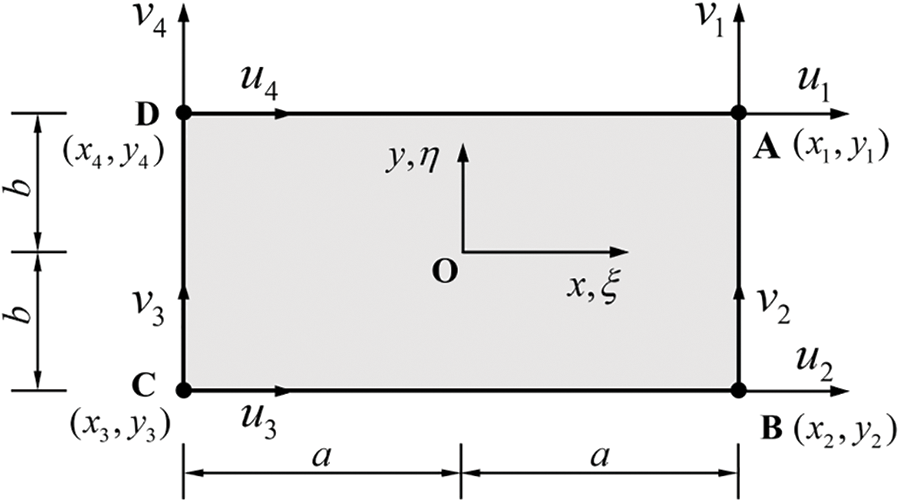
Figure 1: A schematic diagram illustrating a planar four-node rectangular plate element

The displacements at all nodes form a vector qe, expressed as

qe=[u1  v1  u2  v2  u3  v3  u4  v4]T(1)

The element displacement field can then be expressed as

r=Sqe(2)

where S=[S1IS2IS3IS4I] is the matrix functioning as the interpolation function with entries defined by

{S1(x,y)=14(1+ξ)(1+η),S2(x,y)=14(1−ξ)(1+η)S3(x,y)=14(1−ξ)(1−η),S4(x,y)=14(1+ξ)(1−η)(3)

Here, in the rectangular plate element, ξ=x/a and η=y/b represent the dimensionless coordinates, whereas a and b denote the half lengths of the element in the x- and y-directions, respectively.

From the physical equation of the plane problem in elasticity, the stress expression of the plate element is given by

σ=Dε=DBqe=Aqe(4)

where ε is element strain vector, A=DB is the stress function matrix, D is the elastic coefficient matrix for the plane stress problem, B=[B1B2B3B4] is the geometric matrix, expressed as

D=E1−μ2[1μ0μ10001−μ2],Bi=[∂Si∂x00∂Si∂y∂Si∂y∂Si∂x],i=1,2,3,4(5)

In Eq. (5), E represents Young’s modulus and μ is Poisson’s ratio. In the context of this study, they correspond to values of 2.1×105 MPa and 0.3, respectively.

2.2 Analysis of a Cavity Structure

The study conducts topology optimization of two research objects: a circular cavity and a blade section cavity, as shown in Fig. 2. The circular cavity can be used as an engine cavity, high-pressure storage tank, et al. Blade cavities are commonly found in turbine blades [32], propellers [33], et al. The circular cavity consists of a skin and an inner cavity. The geometric configuration can be determined according to the diameter of concentric circles. The blade cavity includes skin, beam, and internal cavity, and its geometry can be obtained by accurate positioning.

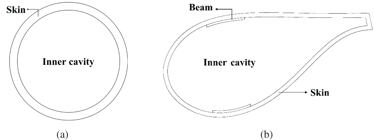
Figure 2: Cavity structures. (a) a circular cavity; (b) a blade cavity

Generally, the blade structure is mainly composed of three parts, that is skin, spar caps, and webs. The positions of blade structural components are given in terms of straight distances and circumferential arc lengths along the cross-sectional contour. Fig. 3 shows these dimensions schematically. The main beams are divided into pressure surface beam and suction surface beam. The pressure surface beam is fitted to the inner side of the pressure surface skin, while the suction surface beam is fitted to the inner side of the suction surface skin. Together, they form the spar caps. There are two parallel supporting webs between the two spars caps.

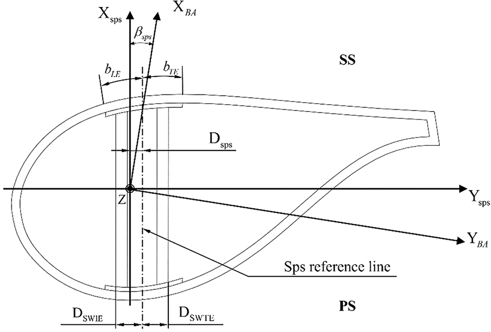
Figure 3: Positioning scheme of rotor blade components

The blade axis COS is an axis parallel to the chord of the reference cross-section. The defined angle βsps in Fig. 3 is the angle between the x-axis of the blade system and the x-axis of the spar cap axis COS for a twist angle. 4.3MW-SR152 rotor blade is selected in this paper, and angle βSps=4∘. The reference line of the spar system (Sps), which consists of the spar cap and the spar web, for details, see Fig. 3, is a straight line between characteristic points defined in relation to the vertical projection of the blade axis. The straight distance DSps is the vertical projection of the spar system reference line onto the blade axis. The beam web structure can be located by the system reference line.

The width of the spar caps is defined by the circumferential arc lengths bLE and bTE. bLE represents the gap between the Sps reference line and the leading edge of the spar cap, while bTE is the distance between the Sps reference line and the trailing edge of the spar cap. The distance between the leading-edge web and the system reference line Sps is DSWLE. The distance between the trailing-edge web and the system reference line Sps is DSWTE. The above parameters vary linearly in the direction of blade length. These design parameters can be used to locate the concrete position of the spar caps and webs at any length of the blade section.

In the blade structure, the section with the largest area is cut off to obtain the blade cavity of the traditional beam web structure. This section is used as a contrast for subsequent stiffness check experiments. Then the two webs in the section are removed, the main beam and skin structure are retained, and the blade cavities are filled. Thus, one of the research objects is obtained: the blade section cavity, as depicted in Fig. 2b.

3  Topology Optimization Formulation

3.1 Density Method

As a sophisticated mathematical methodology, topology optimization methodically calibrates the material distribution within a preordained spatial envelope based on specific load scenarios, constraints, and performance metrics [10,34]. In order to optimize the web layout of the large cavity, this paper employs the variable density method. The design variable, denoted as ρi, represents the density of the i-th finite element. By modifying the value of ρi, it becomes possible to adjust the global structural stiffness and optimize the material arrangement within the structure. The value of ρi corresponds to each of the three cases as follows:

{ρi=0⇔void domain,0<ρi<1⇔intermediate domain,ρi=1⇔material domain.(6)

In general, the smaller the weight, the lower the stiffness. However, when carrying out lightweight design, it is necessary to ensure that the stiffness of the structure does not decrease. Therefore, this paper chooses the flexibility of the structure as the objective function and the volume fraction as the constraint condition so that the influence of the volume fraction on the optimized configuration can also be studied. The stiffness optimization problem is mathematically expressed in the following manner:

minρ:R(ρ)=UTKU=∑i=1N⁡Ei(ρi)uiTk0uis.t.:∑i=1N⁡Viρi−Vf≤0KU=F0≤ρi≤1(7)

where R is the compliance of the cavity structure, N represents the total number of elements, ρ refers to the vector of design variables, U is the global displacement, K is the global stiffness matrices, the element stiffness matrix for an element with a unit Young's modulus is symbolized as k0, the element displacement vector is denoted by ui, Vi is the element volume, Vf corresponds to prescribed volume fraction, F corresponds to the global force vector.

To circumvent the intermediary transition region and enhance the convergence of the binary solution, the relationship between density variables ρi and material properties is elucidated using the SIMP method [30,35] in the following way:

Ei(ρi)=Emin+ρip(E0−Emin)(8)

where p serves as the penalization factor and is empirically established at a value of 3. E0 = 2.1×105 MPa is representative of the material domain. To avoid the stiffness matrix singularity, a void domain is introduced with Emin set to E0×10−8, indicating its negligible material properties.

According to Eqs. (7) and (8), the following expression elucidates the objective function R(ρ):

R(ρ)=∑i=1N⁡[Emin+ρip(E0−Emin)]uiTk0ui(9)

When multiple loading conditions occur, the single-objective optimization is transformed into multi-objective optimization. The mathematical model using the compromise programming method can typically be articulated as follows [36,37]:

min:R(ρ)={∑t=1l⁡wtq[Rt(ρ)−Rtmin(ρ)Rtmax(ρ)−Rtmin(ρ)]q}1qs.t.:∑t=1l⁡(∑i=1N⁡Viρit)−Vf≤0KU=F0≤ρi≤1(10)

where l is the number of loading cases, to establish a square root relationship and determine the weight assigned to each objective, the exponent q, which influences the weight, is set to 2. wt represents the weights of the t-th static working conditions, and the sum of weights of all working conditions is 1. Vi is the element volume for the t-th working environment, Rt(ρ) is the structure compliance of the t-th working environment. Rtmax(ρ) and Rtmin(ρ) are the maximum and minimum values of compliance under the t-th working environment. Firstly, to obtain Rt(ρ) and Rtmin(ρ) for the corresponding loading case, a single-objective optimization problem defined in Eq. (7) is utilized. Then Rtmax(ρ) is obtained by changing the objective function to take the maximum value.

3.2 Sensitivity and Projection

According to Eq. (9), the expressions for the sensitivities of the objective function R(ρ) with regard to a design variable ρi is given as follows [38]:

∂R∂ρi=−pρip−1(E0−Emin)uiTk0ui(11)

For Eq. (10), the sensitivities of the objective function R(ρ) reads

∂R∂ρi=[∑t=1l⁡wtqT(ρ)q]1q−1[∑t=1l⁡wtqT(ρ)q−1∂T∂ρi](12)

where T(ρ), ∂T∂ρi, are respectively represented as

T(ρ)=Rt(ρ)−Rtmin(ρ)Rtmax(ρ)−Rtmin(ρ)∂T∂ρi=∂Rt(ρ)∂ρiRtmax(ρ)−Rtmin(ρ)(13)

Rt(ρ) and ∂Rt(ρ)∂ρi can be calculated from Eqs. (11) and (12), respectively. Rtmax(ρ) and Rtmin(ρ) are calculated from Eqs. (7) and (9), they are two constant terms in Eq. (13).

Topology optimization is often accompanied by mesh dependence and checkerboard. Grid dependence generally means that the minimum size of the optimization configuration depends on the finite element mesh. The checkerboard phenomenon refers to the alternating appearance of entities and voids in the optimal configuration, such as a checkerboard. In order to solve these problems, the general approach entails the utilization of a filtering technique [35,39,40]. The original densities ρi are subjected to a transformation through the density filter, represented as

ρ∼i=1∑e∈Ni⁡Hie∑e∈Ni⁡HieρeHie=max[0,R−Δ(i,e)](14)

where R, defined as treble element size, is denoted as the specified filter radius, within a circular region centered at the e-th element, with a radius of R, Ni represents the collective quantity of elements, Hie is a weight factor, Δ(i,e) represents the distance from the e-th element to the i-th element.

Nevertheless, the application of the filter may introduce gray transition domains characterized by densities between 0 and 1. Too many gray elements will blur the junction between the entity and the void, affecting material recognition. This problem can be resolved by employing the projection technique [41]. The hyperbolic-tangent function form is commonly employed in the projection function, expressed as follows:

ρ^i=H(ρ∼i,η)=tanh⁡(βη)+tanh⁡[β(ρ∼i−η)]tanh⁡(βη)+tanh⁡[β(1−η)](15)

where β serves as the projection parameter controlling the smoothness, typically set to 8, η denotes the projection threshold, typically set to 0.5. For values of ρ∼i exceeding η, the projection results in 1; otherwise, it yields 0. H refers to the projection function, which is convenient for the following statement.

3.3 Member Size Constrain

In this paper, the member size constraints are considered, including the maximum and the minimum member size constraints. The small force transferring paths in the optimization results can be eliminated by the minimum member size constraint, and the minimum size of the structure can be guaranteed to be larger than the minimum member size so as to obtain a relatively uniform material distribution. On the contrary, the maximum member size constraint can provide multiple force-transferring paths and eliminate material stacking in the optimization results. Product defects caused by the manufacturing process, such as the problem of uneven heat dissipation during the casting process, can also be avoided to improve product reliability.

The minimum member size constraint is implemented by proposing two geometric constraints by a three-field scheme [42,43], also known as the filtering-threshold topology optimization scheme. The three fields are formed by filtering and projection transformation of the design field in turn, and the transformation process can be summarized as ρ→ρ∼→ρ^, 0≤ρ≤1. The two geometric constraints are as follows:

gs=1N∑i=1N⁡Iis[min{(ρ∼i−ηe),0}]2≤εgv=1N∑i=1N⁡Iiv[min{(ηd−ρ∼i),0}]2≤ε(16)

where Is=ρ^exp⁡(−c|∇ρ∼|2), Iv=(1−ρ^)exp⁡(−c|∇ρ∼|2). s represents the solid phase. v represents the void phase. ρ∼ is the filtering design field. ρ^ is the projection physical field. ∇ρ∼ is the gradient of the filtered variables. Is and Iv are the structure indicator functions that distinguish solid and void phases by ∇ρ∼. For |∇ρ∼≠0|, c controls the decay rates of Is and Iv. Usually, c=(R/h)4, h represents the element size. For |∇ρ∼=0|, Is=ρ^ and Iv=(1−ρ^). ε is used to compensate for numerical errors, and ε=10−6. When the above geometric constraints are satisfied, the relationship between each threshold is 0<ηd<η<ηe<1.

The maximum member size constraint is based on morphological operators [44], implemented through the erosion and dilation operations, two morphological operations. By erosion operation, solid element sizes smaller than a given structural element will be eliminated. By dilation operation, void element sizes smaller than a given structural element will be eliminated. With Heaviside projections and filtering, both operations can be achieved. The conditions guaranteeing the maximum member size on the solid and void can be written as

∫Ωρ^edx=0∫Ω(1−ρ^d)dx=0(17)

where ρ^d=H(ρ∼,η=0) represents the eroded design. ρ^e=H(ρ∼,η=1) represents the dilated design. Ω is the original physical design field. Thus, two geometric constraints are obtained

ρ^TeV≤ε|V|(1−ρ^d)TV≤ε|V|(18)

where V is the vector of the element volume.

4  Case Studies

4.1 Topology Optimization of a Circular Cavity under Concentrated Load Condition

In this case, the layout optimization of a circular cavity internal web structure under concentrated load condition is studied. As shown in Fig. 4, the outer diameter and skin thickness of the circular cavity are 150 and 7.5 mm, respectively. A pair of concentrated forces F with the same magnitude of 1 N and opposite directions act on the vertices in the y-direction of the cavity.

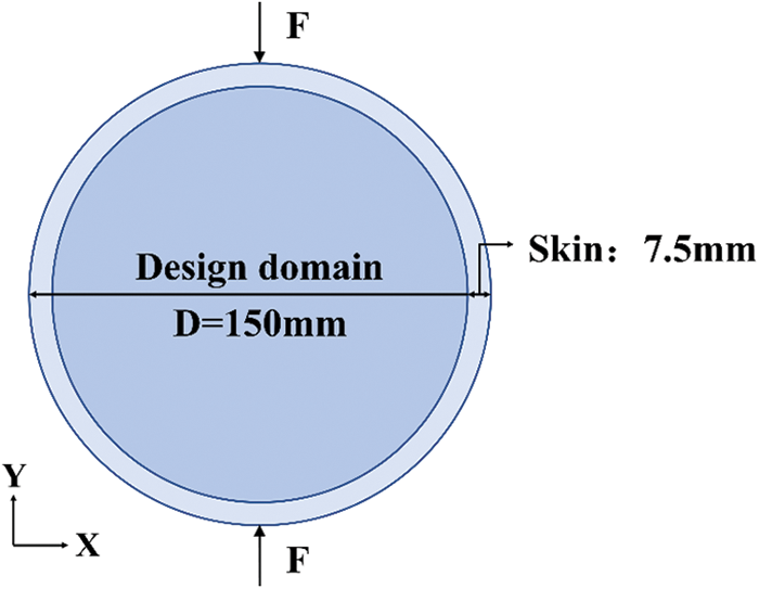
Figure 4: Design domain and boundary conditions

The circular cavity is discretized into 18020 rectangular plate elements with a side length of 1 mm. The material properties of the internal cavity and the skin are identical. The selection of the objective function was guided by the criterion of minimum compliance. A volume fraction of 25% is assigned for Vf. The member size constraints are also considered, where the maximum and minimum member sizes are 12 and 6 mm, respectively.

Fig. 5 presents the optimization result along with the iterative histories of the volume ratio and objective function. The black area represents the material domain, while the white area is the void one. The influence of four factors, that is, mesh size, load magnitude, symmetry constraint, and volume fraction, on the optimization results are investigated, respectively.

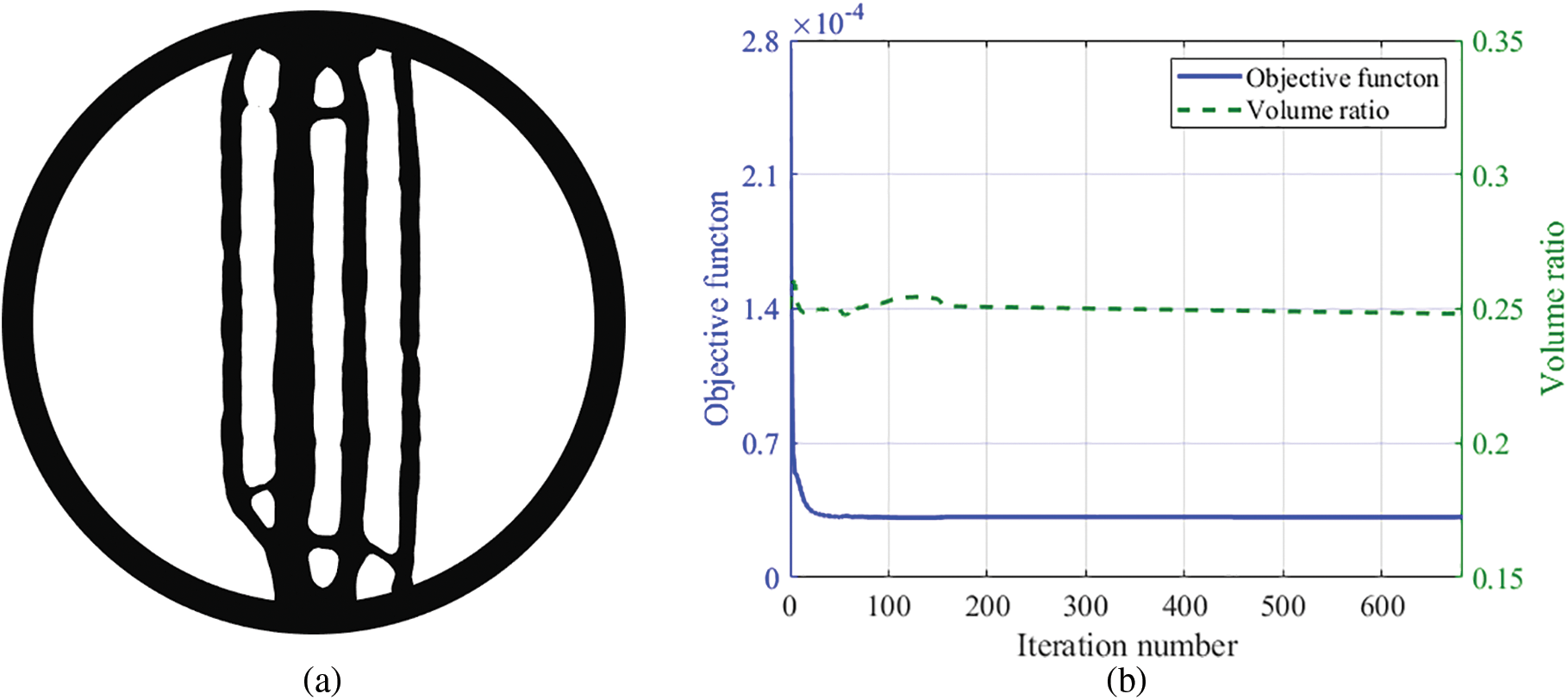
Figure 5: Model with 1 mm element and F = 1 N. (a) Optimization result. (b) Objective function and volume ratio iteration histories

Firstly, an investigation is conducted to explore the influence of mesh size on the optimization results. When employing a side length of 2 mm for the elements, there are 4613 plate elements. The ensuing optimization outcome corresponding to this configuration is visually presented in Fig. 6a, while the iterative histories of the volume ratio and objective function are graphically depicted in Fig. 7a, Figs. 5a and 6a showcase the optimization results, revealing an identical structure that maintains four supporting webs in the y-direction, which retains four supporting webs in the y-direction. As the element size increases, the number of elements decreases, reducing the iteration steps from 749 to 430. Although the 1 mm-size element model has more iteration steps, its optimization result is more refined. The similar converging trends displayed by the volume fraction and objective function corroborate the notion that the mesh size has little impact on the optimization result. With the aim of obtaining more refined results, other subsequent examples in this paper use an element size of 1 mm.

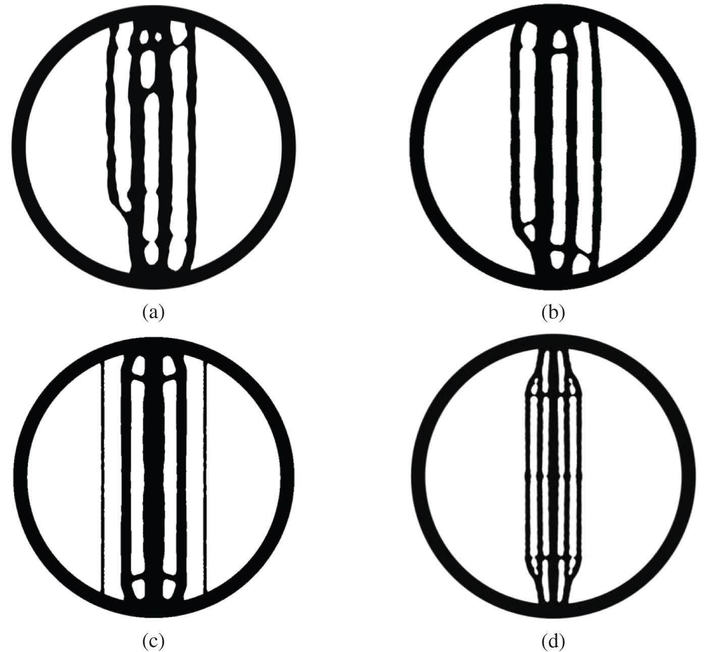
Figure 6: Optimization results. (a) 2 mm-size element, F = 1 N model; (b) 1 mm-mesh element, F = 100 N model; (c) 1 mm-mesh element, F = 1 N, symmetry constraint model; (d) 1 mm-mesh element, F = 1 N, symmetry constraint, Vf = 0.15 model

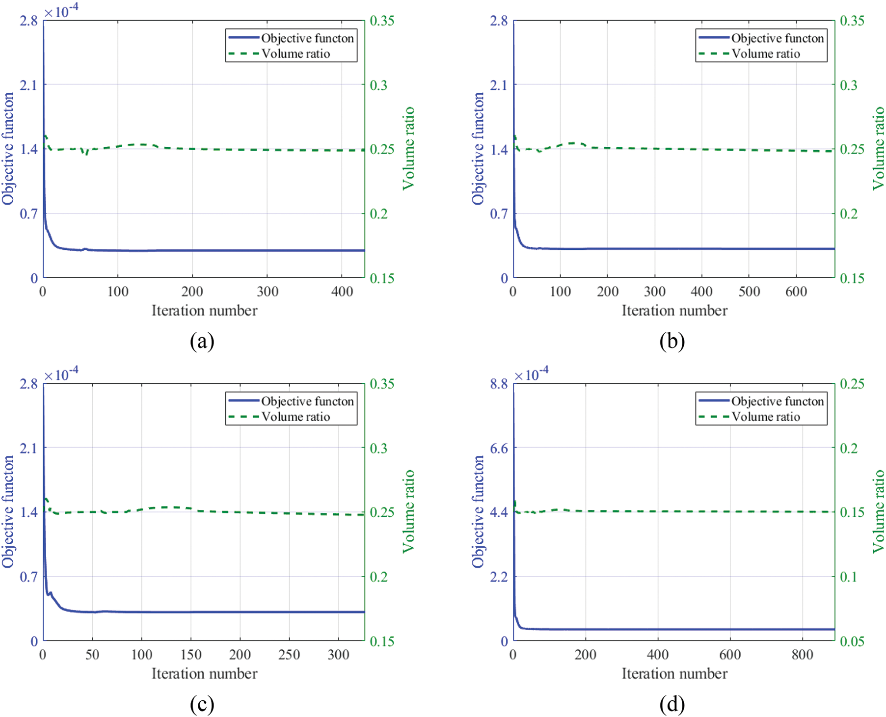
Figure 7: Objective function and volume ratio iteration histories. (a) 2 mm-mesh size element, F = 1 N model; (b) 1 mm-mesh size element, F = 100 N model; (c) 1mm-mesh size element, F = 1 N, symmetry constraint model; (d) 1 mm-mesh size element, F = 1 N, symmetry constraint, Vf = 0.15 model

Secondly, an investigation is conducted to explore the impact of load magnitude on the optimization result. The concentrated force F is set to 100 N for this case. Fig. 6b illustrates the optimization result, while Fig. 7b presents the historical progression of iterations for both the volume ratio and objective function. The optimization results and iteration curves are almost the same as those in Fig. 5. Based on the analysis, it can be inferred that the optimization model remains relatively unaffected by variations in the magnitude of the applied load. To facilitate result comparison, the load magnitude is normalized. In the following examples, the load magnitude is set as 1 N.

Thirdly, to examine the impact of a symmetric constraint on the optimization results and facilitate industrial manufacturing, symmetry constraint is incorporated into the optimization outcome. The final result mandates symmetry around both the x-z and the y-z plane as a fundamental requirement. Fig. 6c delineates the optimization results, whereas Fig. 7c depicts the iterative progression for both the volume ratio and the objective function of the progression of iteration curves. Compared with Fig. 5a, the supporting webs in Fig. 6c are straight and uniform in thickness. However, on either side, there are two straight narrow webs whose dimensions are less than the optimized minimum size. This is the result of the projection technique eliminating many elements with densities less than 0.5.

Fourth, to eliminate these two narrow webs and further reduce the weight, the volume fraction is reduced to 15%. At the same time, the maximum and minimum member sizes are adjusted to 6 and 3 mm. Fig. 6d delineates the optimization results, whereas Fig. 7d provides a detailed depiction of the iterative progression for both the volume ratio and the objective function. In the results, the number of webs increased to 5, and the arrangement is symmetrical. The slender webs vanish, while the volume fraction effectively satisfies the imposed volume constraint.

For the purpose of authenticating the correctness of the optimization results, the ABAQUS software has been employed to compute the displacement and stress of the model both before and after optimization. Since the volume fraction constraint during topology optimization is set as 0.15, to ensure the same mass of the two structures before and after optimization, the thicknesses of the optimized and the unoptimized structures are set to be 1 and 0.15 mm, respectively.

Under the same mass condition, the optimized circular cavity structure demonstrates substantial enhancement in mechanical properties, as indicated by the results. Table 1 and Fig. 8 collectively exhibit the results of mechanical analysis for the two structures when subjected to a concentrated force. The unoptimized structure exhibits a maximum stress of 2.632 MPa, along with a maximum displacement of 5.323 × 10−5 mm. After optimization, the maximum stress is 0.786 MPa, and the maximum displacement is 3.133 × 10−5 mm. The loading point of the unoptimized structure manifests evident stress concentration and substantial displacement. Through optimization, the stress concentration at the loading point is effectively mitigated, with maximum stress reduced by 70.13%. The structure achieves a significant 41.14% reduction in maximum displacement. Under the same mass condition, the optimized circular cavity structure demonstrates substantial enhancement in mechanical properties, as indicated by the results.

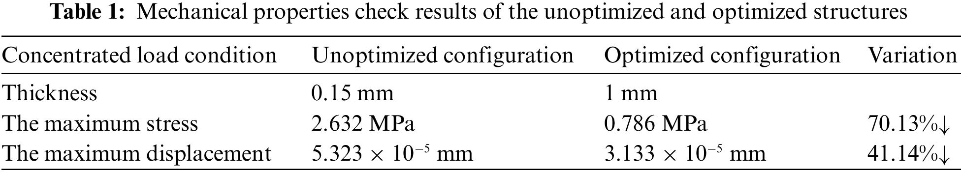
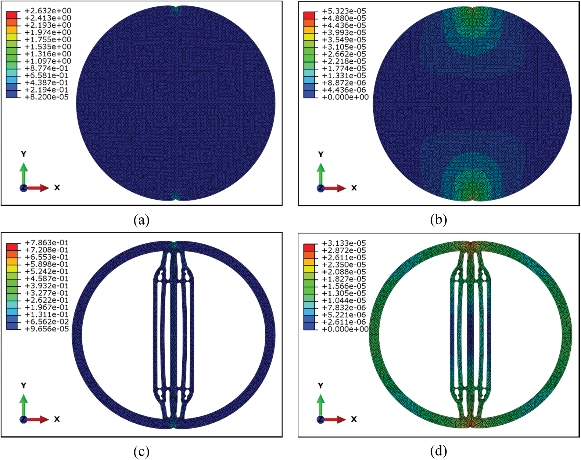
Figure 8: Mechanical properties check results. (a) Unoptimized configuration’s stress nephogram; (b) Unoptimized configuration’s displacement nephogram; (c) Optimized configuration's stress nephogram; (d) Optimized configuration’s displacement nephogram

4.2 Topology Optimization of a Circular Cavity under Uniform Load Condition

In this case, the layout optimization of the web structure of a circular cavity under the uniform load is studied. The concentrated load F is transformed into the uniformly distributed load q. The value of q satisfies the formula.

F=ql(19)

where l is the arc length in the load range, this loading mode is closer to the force situation of the cavity structure in actual work, which is shown in Fig. 9.

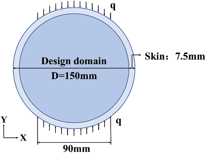
Figure 9: Design domain and boundary conditions

The volume constraint equals 0.25. The member size constraints are also considered, with the maximum and minimum member sizes being 12 and 6 mm, respectively.

Fig. 10a displays the optimization result, while Fig. 11a provides a detailed depiction of the iterative progression for both the volume ratio and the objective function. With the expansion of the force's loading range in the x-direction, a supportive structure oriented within the same axis emerges in the optimization result. The y-direction support structure presents a complex and disordered network structure. According to the volume fraction iteration curve, the optimization result satisfies the volume constraint.

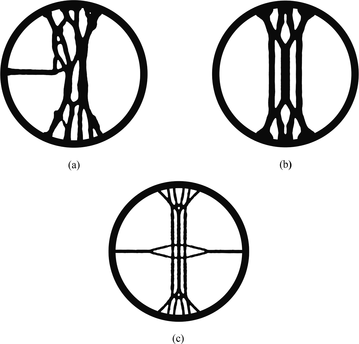
Figure 10: Optimization results. (a) 1 mm-size element, qn = 1 N, model; (b) 1 mm-size element, qn = 1 N, symmetry constraint model; (c) 1 mm-size element, qn = 1 N, symmetry constraint, Vf = 0.15 model

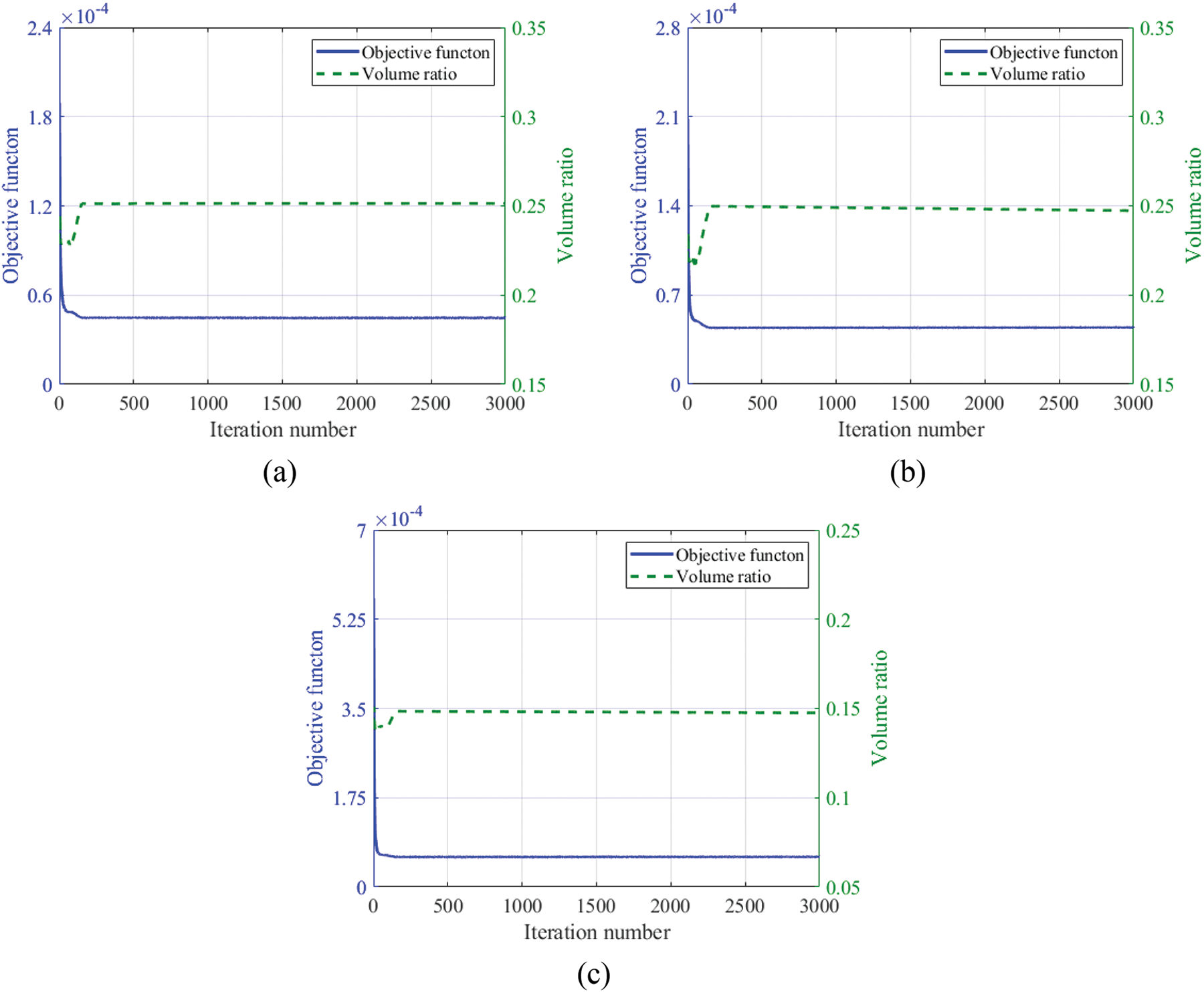
Figure 11: Objective function and volume ratio iteration histories. (a) 1 mm-size element, qn = 1 N, symmetry constraint model; (b) 1 mm-size element, qn = 1 N, symmetry constraint model; (c) 1 mm-size element, qn = 1 N, symmetry constraint, Vf = 0.15 model

In order to facilitate industrial manufacturing, the symmetric constraint is considered. Fig. 10b presents the optimization results, while Fig. 11b provides a detailed depiction of the iterative progression for both the volume ratio and the objective function. Compared with Fig. 10a, the web in the y-direction in Fig. 10b is missing. Prior to the disordered network, the structure is effectively eliminated, making the overall structure more symmetrical. It is helpful to ease production and manufacturing challenges.

For the purpose of weight reduction, the volume fraction parameter of 0.15 has been set. Accordingly, the maximum and the minimum member size are set as 6 and 3 mm. The optimization result and convergence profiles of the volume ratio and objective function are visualized in Figs. 10c and 11c, respectively. The result indicates a symmetric arrangement of the web. A new web layout of the optimization result consists of three vertical webs and one horizontal web. The volume fraction meets the volume constraint.

The optimization results depicted in Fig. 10c have undergone an examination of their mechanical properties. To ensure the same weight for the two structures, the thickness of the optimized and unoptimized structures are set as 1 and 0.15 mm, respectively. The mechanical performance of the optimized cavity structure can be verified by comparing the displacement and stress distribution of two cavity structures under the same load q.

The simulation results of the unoptimized and optimized structures are shown in, thereby enhancing the overall structural stiffness of the cavity.

The unoptimized structure exhibits a maximum stress of 0.114 MPa and a vertex displacement in the y-direction of 3.133 × 10−5 mm. After optimization, the maximum stress is 0.095 MPa. The vertex has experienced a displacement of 1.992 × 10−5 mm in the y-direction. The maximum stress is reduced by 17.15%, and the displacement of the vertex is reduced by 17.17% in Table 2. The results in Fig. 12 indicate that the horizontal and vertical webs effectively inhibit the displacement of the cavity, thereby enhancing the overall structural stiffness of the cavity.

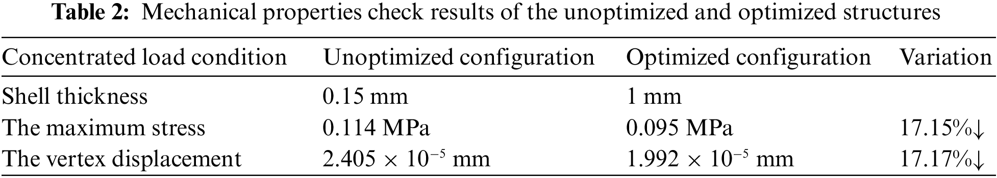
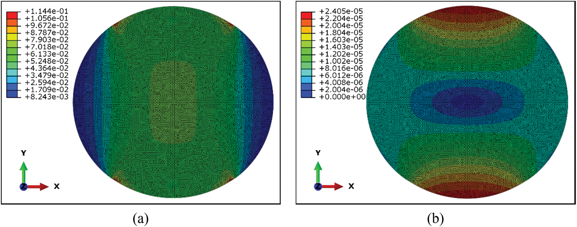
Figure 12: Mechanical properties check results. (a) Unoptimized configuration stress nephogram; (b) Unoptimized configuration displacement nephogram; (c) Optimized configuration stress nephogram; (d) Optimized configuration displacement nephogram

4.3 Topology Optimization of a Blade Cavity for Web Layout Design

In order to provide a new structure with a more robust web layout in the blade cavity, this case takes the blade cavity as the research object and studies the layout optimization of the web structure in the blade cavity. Fig. 13 illustrates the conventional beam web arrangement and the corresponding design domain. The blade airfoil is SR152, with a chord length of 150 mm. The thickness of blade skin and spar caps are 3 and 1.5 mm. The spar caps width equals the sum of bLE and bTE, that is, 27 mm. The skin and inner cavity share the same material composition, with the inner cavity being considered the design domain.

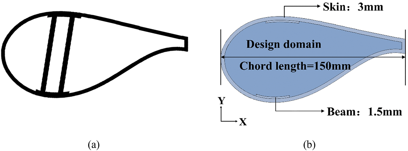
Figure 13: Blade model. (a) Traditional beam web structure blade cavity; (b) Design domain

According to the results in Section 4.1, the element size is 1 mm, so 15,459 plate elements are used to discretize the blade cavity structure. The turbulence model Spalart-Allmaras [45] can be calculated to get the pressure distribution on the airfoil section. When the installation angle of the blade is 12 degrees, the pressure curve of the suction and pressure side is shown in Fig. 14. The pressure on both sides is divided into two working conditions, shown in Fig. 15. In the condition I, the suction side beam is immobilized and the load is imposed on the pressure side. In contrast, in condition II, the pressure side beam is immobilized and the load is imposed on the suction side. The minimum weighted compliance for the two conditions is the objective function with the convergence tolerance ratio of 1×10−8. The compliance value is defined as the weighted sum of the compliance values under two working conditions. The weighted ratios for the two conditions are both 0.5.

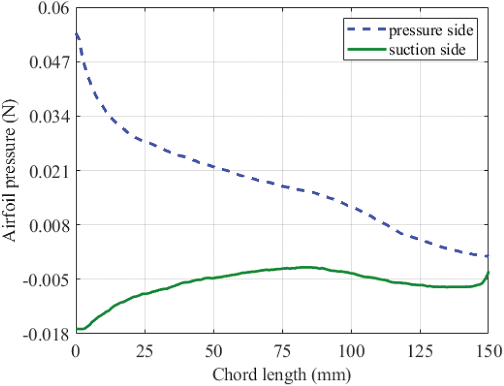
Figure 14: Loading curve of the blade

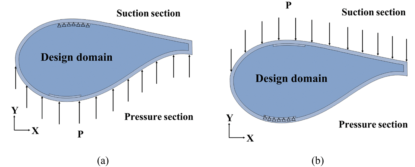
Figure 15: Blade loading condition. (a) Condition I; (b) Condition II

Considering the conventional blade cavity web structure, Vf=0.1 is the volume fraction set to ensure the same weight before and after optimization. Member size constraints are also considered, with the maximum and the minimum member size being 6 and 3 mm.

As illustrated in Fig. 16, the optimization results without and with symmetric constraints. Fig. 17 depicts the histories of the volume ratio and objective function iterations. Fig. 16a, irregular web structures differ from traditional web layouts. The web structures are mainly concentrated in the middle part of the cavity. Like the traditional web layout, no web is at the trailing edge. After adding the symmetric constraint, in Fig. 16b, the structure presents a relatively novel symmetrical network layout. The webs in chord direction, vertical direction, and 45° angle with vertical direction appear simultaneously. Fig. 17 shows that the results satisfy the volume constraint after convergence.

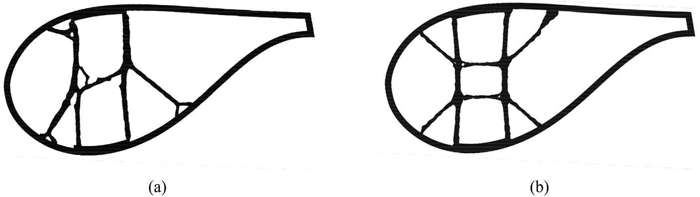
Figure 16: Optimization results. (a) Without symmetry constraint model; (b) With symmetry constraint model

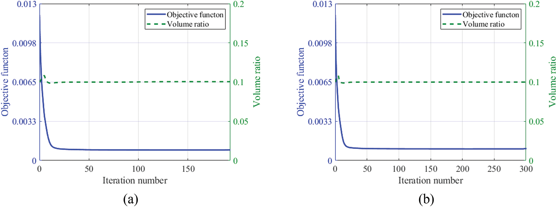
Figure 17: Objective function and volume ratio iteration histories. (a) Without symmetry constraint model; (b) With symmetry constraint model

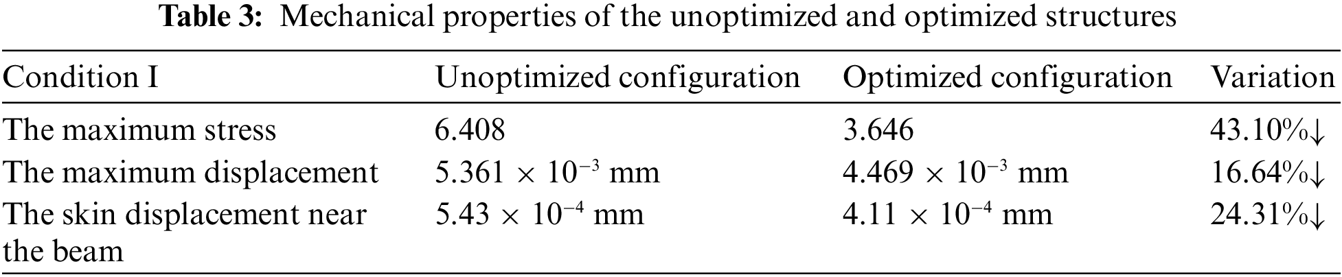
As shown in Figs. 18 and 19, the mechanical simulation results of the unoptimized model and the optimized model under two working conditions are presented. In the condition I, Table 3, the detailed data, the unoptimized model exhibits a maximum stress of 6.408 MPa and a maximum displacement of 5.361 × 10−3 mm. The optimized model exhibits a maximum stress of 3.646 MPa and a maximum displacement of 4.469 × 10−3 mm. The maximum stress and displacement decrease by 43.1% and 16.64%, respectively. Compared with Figs. 18a, 18b, 19a, and 19b, the stress on the skin exhibits improved uniformity after optimization. The stress concentration is effectively relieved. The skin displacement near the pressure side beam before and after optimization are 5.43 × 10−4 mm and 4.11 × 10−4 mm, respectively, and the displacement is reduced by 24.31%.

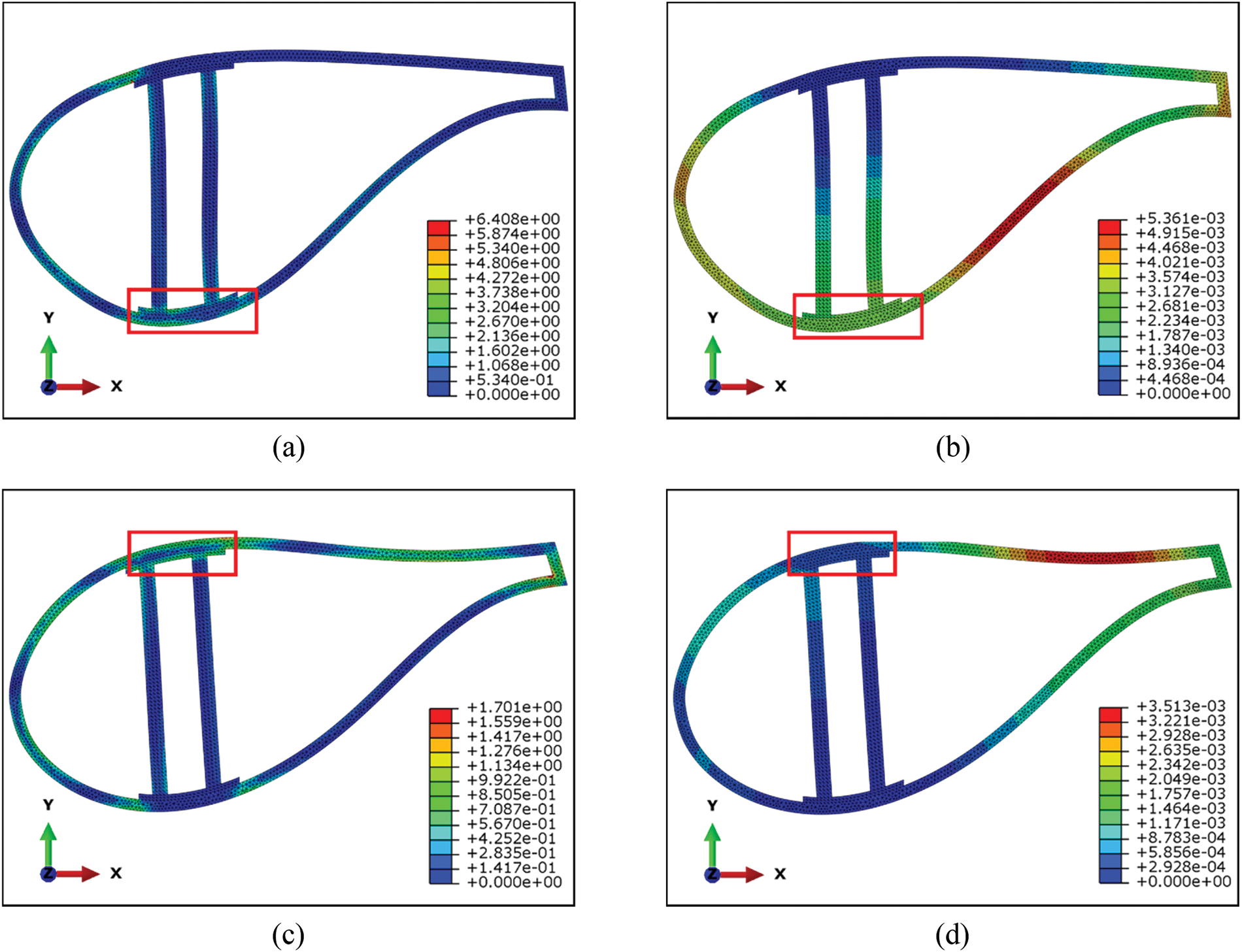
Figure 18: Mechanical properties check of the unoptimized model. (a) The stress nephogram of condition I; (b) The displacement nephogram of condition I; (c) The stress nephogram of condition II; (d) The displacement nephogram of condition II

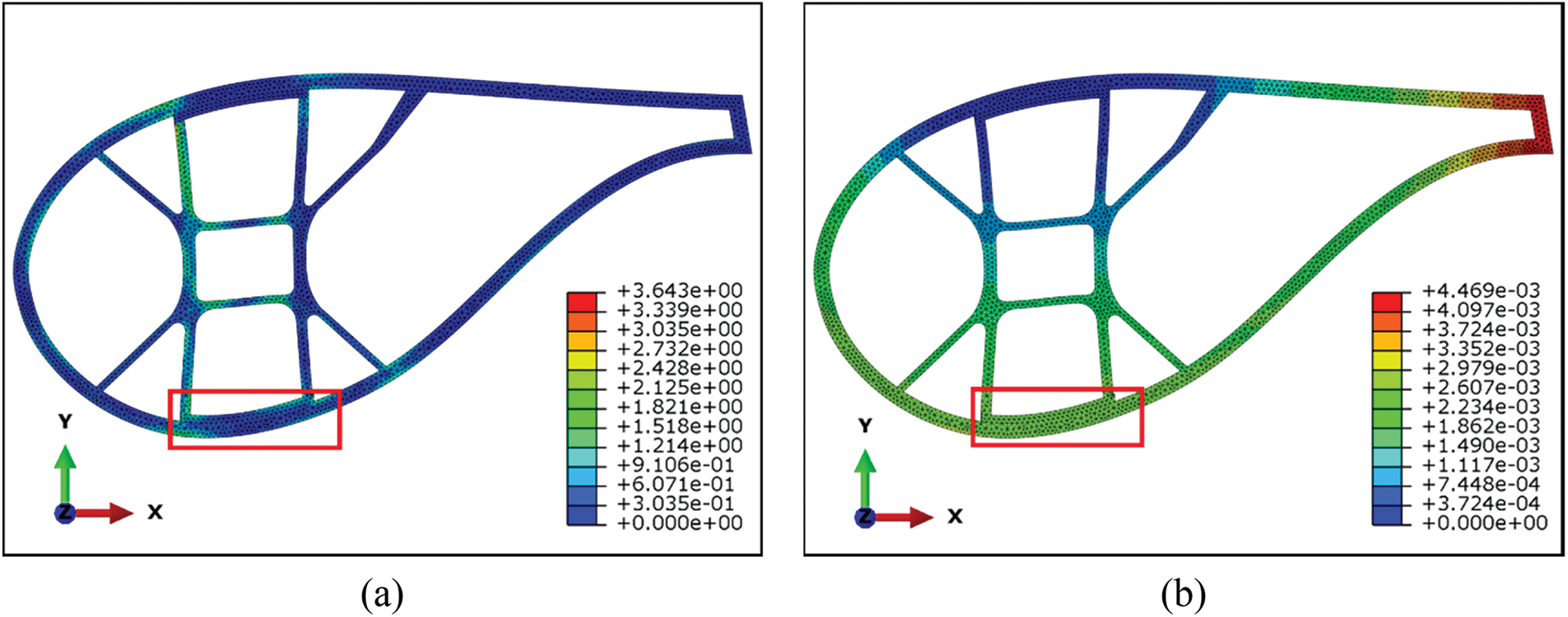
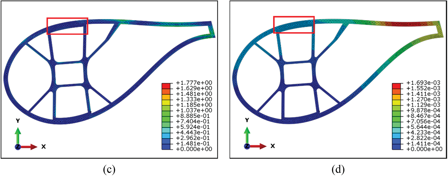
Figure 19: Mechanical properties check of the optimized model. (a) The stress nephogram of condition I; (b) The displacement nephogram of condition I; (c) The stress nephogram of condition II; (d) The displacement nephogram of condition II

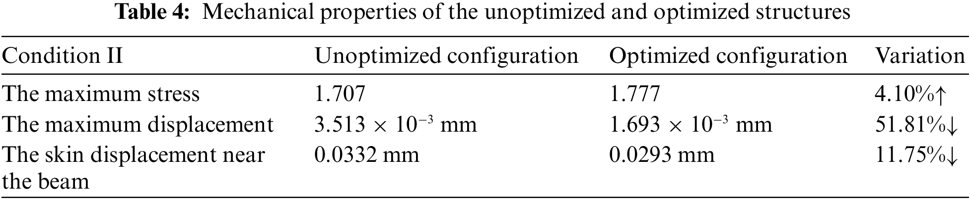
In condition II, Table 4, the detailed data, the maximum stress, and the maximum displacement of the unoptimized model are 1.707 MPa and 3.513 × 10−3 mm. In the optimized model, maximum displacement and maximum stress are 1.777 MPa and 1.693 × 10−3 mm, respectively. However, the maximum stress increases by 4.1%, Figs. 18c, 18d, 19c and 19d demonstrate that the load acting on the pressure side is better transmitted to the web, which also significantly reduces the displacement of the blade. The maximum displacement is reduced by 51.81%. The skin displacement near the suction side beam before and after optimization is 0.0332 and 0.0293 mm respectively, which decreased by 11.75% after optimization. The results demonstrate a substantial enhancement in the mechanical properties of the blade cavity under both condition I and condition II.

5  Conclusion

In this paper, the web layout design of large cavity structures based on topology optimization is carried out. Detailed topology of the large cavity structures is described using SIMP. By using element densities as design variables, the web layouts are optimized for circular and blade cavities by minimizing structural compliance and constraining volume fraction. Optimizing the circular cavity structure involves investigating two load conditions: concentrated and distributed loads. Additionally, the influence of mesh size, load magnitude, symmetry constraint, and volume fraction on the optimization results is explored. The findings reveal that mesh size and load magnitude have negligible influence on the optimized configuration. Symmetry constraints can make the result more beneficial to put into production. The reduction of volume fraction can further reduce the structural weight. The optimized design model is established according to the design parameters of a commercial 4.3MW-SR152 blade. The optimized result shows that the web layout differs from the traditional ones with webs in chord direction, vertical direction, and 45° angle with vertical direction appearing simultaneously. The mechanical properties of the structures before and after optimization are compared. It reveals that the optimized structure is stiffer than its unoptimized counterpart while maintaining the same mass, with varying degrees of improvement. For the circular cavity, the maximum displacement is reduced by 41.14% in the concentrated load case, and the vertex displacement is reduced by 17.17% in the uniformly distributed force case. The maximum displacement of the blade cavity structure is reduced by 51.81% in condition I and 16.64% in condition II, respectively. In addition, stress concentration is also relieved with the maximum stress of the circular cavity structure reduced by 70.13% in the concentrated load case and 17.15% in the uniformly distributed force case. In condition II, a notable 43.1% reduction is observed in the maximum stress of the blade cavity structure.

Acknowledgement: This paper’s logical organisation and content quality have been enhanced, so the authors thank anonymous reviewers and journal editors for assistance.

Funding Statement: This work was supported in part by the National Natural Science Foundation of China and the Natural Science Foundation of Jiangsu Province. It was also supported in part by Young Elite Scientists Sponsorship Program by CAST.

Author Contributions: The authors confirm contribution to the paper as follows: study conception and design: Xiaoqiao Yang, Jialiang Sun, data collection: Xiaoqiao Yang, analysis and interpretation of results: Xiaoqiao Yang, Jialiang Sun, draft manuscript preparation: Xiaoqiao Yang, Jialiang Sun and Dongping Jin. All authors reviewed the results and approved the final version of the manuscript.

Availability of Data and Materials: The data that support the findings of this study are available from the first and corresponding authors upon reasonable request.

Conflicts of Interest: The authors declare that they have no conflicts of interest to report regarding the present study.

References

1. Soutis, C. (2005). Carbon fiber reinforced plastics in aircraft construction. Materials Science and Engineering: A, 412(1–2), 171–176. https://doi.org/10.1016/j.msea.2005.08.064 [Google Scholar] [CrossRef]

2. Gürbüz, H., Akçay, H., Aldemir, M., Akçay, İ. H., Topalcı, Ü. (2021). The effect of euro diesel-hydrogen dual fuel combustion on performance and environmental-economic indicators in a small UAV turbojet engine. Fuel, 306(2), 121735. https://doi.org/10.1016/j.fuel.2021.121735 [Google Scholar] [CrossRef]

3. Stein, M. (2003). Some recent advances in the investigation of shell buckling. Journal of Spacecraft and Rockets, 40(6), 908–917. https://doi.org/10.2514/2.7057 [Google Scholar] [CrossRef]

4. Noor, A. K., Venneri, S. L., Paul, D. B., Hopkins, M. A. (2000). Structures technology for future aerospace systems. Computers & Structures, 74(5), 507–519. https://doi.org/10.1016/S0045-7949(99)00067-X [Google Scholar] [CrossRef]

5. Vasiliev, V. V., Razin, A. F. (2006). Anisogrid composite lattice structures for spacecraft and aircraft applications. Composite Structures, 76(1–2), 182–189. https://doi.org/10.1016/j.compstruct.2006.06.025 [Google Scholar] [CrossRef]

6. Jin, D., Bin, J. (2015). Topology optimization of flexible support structure for trailing edge. Acta Aeronautica et Astronautica Sinica in Chinese, 36(8), 2681–2687. https://doi.org/10.7527/S1000-6893.2015.0105 [Google Scholar] [CrossRef]

7. Cavallaro, R., Demasi, L. (2016). Challenges, ideas, and innovations of joined-wing configurations: A concept from the past, an opportunity for the future. Progress in Aerospace Sciences, 87(3), 1–93. https://doi.org/10.1016/j.paerosci.2016.07.002 [Google Scholar] [CrossRef]

8. Guerder, M., Duval, A., Elguedj, T., Feliot, P., Touzeau, J. (2022). Isogeometric shape optimisation of volumetric blades for aircraft engines. Structural and Multidisciplinary Optimization, 65(3), 1–17. https://doi.org/10.1007/s00158-021-03090-z [Google Scholar] [CrossRef]

9. Bendsoe, M. P., Kikuchi, N. (1988). Generating optimal topologies in structural design using a homogenization method. Computer Methods in Applied Mechanics and Engineering, 71(2), 197–224. https://doi.org/10.1016/0045-7825(88)90086-2 [Google Scholar] [CrossRef]

10. Sigmund, O., Maute, K. (2013). Topology optimization approaches: A comparative review. Structural and Multidisciplinary Optimization, 48(6), 1031–1055. https://doi.org/10.1007/s00158-013-0978-6 [Google Scholar] [CrossRef]

11. Bendsøe, M. P. (1989). Optimal shape design as a material distribution problem. Structural Optimization, 1(4), 193–202. https://doi.org/10.1007/BF01650949 [Google Scholar] [CrossRef]

12. Mlejnek, H. P. (1992). Some aspects of the genesis of structures. Structural Optimization, 5(1–2), 64–69. https://doi.org/10.1007/BF01744697 [Google Scholar] [CrossRef]

13. Xie, Y. M., Steven, G. P. (1993). A simple evolutionary procedure for structural optimization. Computers & Structures, 49(5), 885–896. https://doi.org/10.1016/0045-7949(93)90035-C [Google Scholar] [CrossRef]

14. Xie, Y. M. (2022). Generalized topology optimization for architectural design. Architectural Intelligence, 1(1), 1–11. https://doi.org/10.1007/s44223-022-00003-y [Google Scholar] [CrossRef]

15. Allaire, G., Jouve, F., Toader, A. M. (2002). A level-set method for shape optimization. Comptes Rendus Mathematique, 334(12), 1125–1130. https://doi.org/10.1016/S1631-073X(02)02412-3 [Google Scholar] [CrossRef]

16. Yu, C., Wang, Q., Mei, C., Xia, Z. (2020). Multiscale isogeometric topology optimization with unified structural skeleton. Computer Modeling in Engineering & Sciences, 122(3), 779–803. https://doi.org/10.32604/cmes.2020.09363 [Google Scholar] [CrossRef]

17. Wang, Y., Kang, Z. (2021). MATLAB implementations of velocity field level set method for topology optimization: An 80-line code for 2D and a 100-line code for 3D problems. Structural and Multidisciplinary Optimization, 64(6), 4325–4342. https://doi.org/10.1007/s00158-021-02958-4 [Google Scholar] [CrossRef]

18. Bourdin, B., Chambolle, A. (2003). Design-dependent loads in topology optimization. ESAIM: Control. Optimisation and Calculus of Variations, 9, 247–273. https://doi.org/10.1051/cocv:2002070 [Google Scholar] [CrossRef]

19. Guo, X., Zhou, J., Zhang, W., Du, Z., Liu, C. et al. (2017). Self-supporting structure design in additive manufacturing through explicit topology optimization. Computer Methods in Applied Mechanics and Engineering, 323, 27–63. https://doi.org/10.1016/j.cma.2017.05.003 [Google Scholar] [CrossRef]

20. Zhang, W., Zhou, J., Zhu, Y., Guo, X. (2017). Structural complexity control in topology optimization via moving morphable component (MMC) approach. Structural and Multidisciplinary Optimization, 56(3), 535–552. https://doi.org/10.1007/s00158-017-1736-y [Google Scholar] [CrossRef]

21. Zhang, W., Yang, W., Zhou, J., Li, D., Guo, X. (2017). Structural topology optimization through explicit boundary evolution. Journal of Applied Mechanics, 84(1), 1–10. https://doi.org/10.1115/1.4034972 [Google Scholar] [CrossRef]

22. Zhang, W., Chen, J., Zhu, X., Zhou, J., Xue, D. et al. (2017). Explicit three dimensional topology optimization via moving morphable void (MMV) approach. Computer Methods in Applied Mechanics and Engineering, 322(1), 590–614. https://doi.org/10.1016/j.cma.2017.05.002 [Google Scholar] [CrossRef]

23. Sun, J., Tian, Q., Hu, H., Pedersen, N. L. (2019). Topology optimization for eigenfrequencies of a rotating thin plate via moving morphable components. Journal of Sound and Vibration, 448(1), 83–107. https://doi.org/10.1016/j.jsv.2019.01.054 [Google Scholar] [CrossRef]

24. Lee, S. L., Shin, S. J. (2022). Structural design optimization of a wind turbine blade using the genetic algorithm. Engineering Optimization, 54(12), 2053–2070. https://doi.org/10.1080/0305215X.2021.1973450 [Google Scholar] [CrossRef]

25. Félix, L., Gomes, A. A., Suleman, A. (2020). Topology optimization of the internal structure of an aircraft wing subjected to self-weight load. Engineering Optimization, 52(7), 1119–1135. https://doi.org/10.1080/0305215X.2019.1639691 [Google Scholar] [CrossRef]

26. Wang, Q., Hong, X., Qin, Z. Z., Wang, J., Sun, J. F. et al. (2017). Topology optimal design of wind turbine blades considering aerodynamic load. 3rd Annual 2017 International Conference on Sustainable Development, 111, 211–216. https://doi.org/10.2991/icsd-17.2017.33 [Google Scholar] [CrossRef]

27. Jensen, P. D. L., Wang, F., Dimino, I., Sigmund, O. (2021). Topology optimization of large-scale 3D morphing wing structures. Actuators, 10(9), 1–16. https://doi.org/10.3390/act10090217 [Google Scholar] [CrossRef]

28. Elelwi, M., Calvet, T., Botez, R. M., Dao, T. M. (2021). Wing component allocation for a morphing variable span of tapered wing using finite element method and topology optimisation—Application to the UAS-S4. Aeronautical Journal, 125(1290), 1313–1336. https://doi.org/10.1017/aer.2021.29 [Google Scholar] [CrossRef]

29. Aage, N., Andreassen, E., Lazarov, B. S., Sigmund, O. (2017). Giga-voxel computational morphogenesis for structural design. Nature, 550(7674), 84–86. https://doi.org/10.1038/nature23911 [Google Scholar] [PubMed] [CrossRef]

30. Sun, J., Jin, D., Hu, H. (2022). Deployment dynamics and topology optimization of a spinning inflatable structure. Acta Mechanica Sinica, 38, 122100 (In Chinese). https://doi.org/10.1007/s10409-022-22100-x [Google Scholar] [CrossRef]

31. Sun, Z., Wang, Y., Gao, Z., Luo, Y. (2023). Topology optimization of thin-walled structures with directional straight stiffeners. Applied Mathematical Modelling, 113(1), 640–663. https://doi.org/10.1016/j.apm.2022.09.027 [Google Scholar] [CrossRef]

32. Luo, Y., Wen, F., Wang, S., Zhang, S., Wang, S. et al. (2019). Numerical investigation on the biomimetic trailing edge of a high-subsonic turbine blade. Aerospace Science and Technology, 89(1), 230–241. https://doi.org/10.1016/j.ast.2019.04.002 [Google Scholar] [CrossRef]

33. Hussain, M., Abdel-Nasser, Y., Banawan, A., Ahmed, Y. M. (2020). FSI-based structural optimization of thin bladed composite propellers. Alexandria Engineering Journal, 59(5), 3755–3766. https://doi.org/10.1016/j.aej.2020.06.032 [Google Scholar] [CrossRef]

34. Wang, Y., Li, X., Long, K., Wei, P. (2023). Open-source codes of topology optimization: A summary for beginners to start their research. Computer Modeling in Engineering & Sciences, 137(1), 1–34. https://doi.org/10.32604/cmes.2023.027603 [Google Scholar] [CrossRef]

35. Andreassen, E., Clausen, A., Schevenels, M., Lazarov, B. S., Sigmund, O. (2011). Efficient topology optimization in MATLAB using 88 lines of code. Structural and Multidisciplinary Optimization, 43(1), 1–16. https://doi.org/10.1007/s00158-010-0594-7 [Google Scholar] [CrossRef]

36. Luo, Z., Yang, J., Chen, L. P., Zhang, Y. Q., Abdel-Malek, K. (2006). A new hybrid fuzzy-goal programming scheme for multi-objective topological optimization of static and dynamic structures under multiple loading conditions. Structural and Multidisciplinary Optimization, 31(1), 26–39. https://doi.org/10.1007/s00158-005-0543-z [Google Scholar] [CrossRef]

37. Luo, Z., Chen, L. P., Yang, J., Zhang, Y. Q. (2006). Multiple stiffness topology optimizations of continuum structures. International Journal of Advanced Manufacturing Technology, 30(3–4), 203–214. https://doi.org/10.1007/s00170-005-0084-z [Google Scholar] [CrossRef]

38. Sigmund, O. (2001). A 99 line topology optimization code written in Matlab. Structural and Multidisciplinary Optimization, 21(2), 120–127. http://www.topopt.dtu.dk [Google Scholar]

39. Svanberg, K. (1987). The method of moving asymptotes—A new method for structural optimization. International Journal for Numerical Methods in Engineering, 24(2), 359–373. https://doi.org/10.1002/(ISSN)1097-0207 [Google Scholar] [CrossRef]

40. Sigmund, O. (2007). Morphology-based black and white filters for topology optimization. Structural and Multidisciplinary Optimization, 33(4–5), 401–424. https://doi.org/10.1007/s00158-006-0087-x [Google Scholar] [CrossRef]

41. Wang, F., Lazarov, B. S., Sigmund, O. (2011). On projection methods, convergence and robust formulations in topology optimization. Structural and Multidisciplinary Optimization, 43(6), 767–784. https://doi.org/10.1007/s00158-010-0602-y [Google Scholar] [CrossRef]

42. Lazarov, B. S., Wang, F., Sigmund, O. (2016). Length scale and manufacturability in density-based topology optimization. Archive of Applied Mechanics, 86(1–2), 189–218. https://doi.org/10.1007/s00419-015-1106-4 [Google Scholar] [CrossRef]

43. Zhou, M., Lazarov, B. S., Wang, F., Sigmund, O. (2015). Minimum length scale in topology optimization by geometric constraints. Computer Methods in Applied Mechanics and Engineering, 293, 266–282. https://doi.org/10.1016/j.cma.2015.05.003 [Google Scholar] [CrossRef]

44. Lazarov, B. S., Wang, F. (2017). Maximum length scale in density based topology optimization. Computer Methods in Applied Mechanics and Engineering, 318(2), 826–844. https://doi.org/10.1016/j.cma.2017.02.018 [Google Scholar] [CrossRef]

45. Mittal, S., De, A., Kumar, V. (2006). Finite element computation of turbulent flow past a multi-element airfoil. International Journal of Computational Fluid Dynamics, 20(8), 563–577. https://doi.org/10.1080/10618560601046960 [Google Scholar] [CrossRef]