A Novel Predictive Model for Edge Computing Resource Scheduling Based on Deep Neural Network

1  Introduction

The evolution of the mobile Internet has enabled applications to access cloud data centers for remote computing resources. In smart cities and smart factories, data generated by sensors and end-devices (e.g., smartphones and wearables) are transmitted over the network to remote cloud computing centers for processing and storage. This operational process, nevertheless, potentially increases communication time dramatically, thereby reducing the overall quality of experience (QoE) and quality of service (QoS) for the user. While showing numerous advantages, cloud computing brings a new set of problems, such as data latency and high data traffic caused by the multitude of mobile devices, affecting both latency-sensitive and time-sensitive applications [1,2]. In addition, the rapid development of multimedia services has led to an increasing demand for network bandwidth from mobile devices, making mobile network capacity and backhaul links a critical challenge. To address the aforementioned issues and reduce communication latency, Mobile Edge Computing (MEC) has emerged to frontload cloud resources and services to the edge nodes (base stations) closest to mobile devices and become a cost-effective solution with low latency [3].

MEC provides time-intensive and compute-intensive application services to mobile devices by extending compute along with storage resources to the edge of the mobile network adjacent to the mobile terminals and deploying applications on mobile edge servers. The MEC architecture significantly reduces congestion in the central network and significantly improves quality of experience (QoE) and quality of service (QoS) by meeting stringent requirements for response latency. Surely, MEC inherently also has some limitations, including network bandwidth, CPU resources and, memory resources, etc. Therefore, an efficient resource management system is extremely important for MEC to perform real functions. At the present stage, the research focuses more on task offloading, optimizing application deployment, reducing power consumption of terminal devices and allocating computing resources for MEC. Although the existing research works promoted the development of MEC, the absence of considering the different demands for resource allocation in different time periods is their common limitation. The Edge computing system model structure is shown in Fig. 1. Edge computing is widely recognized as a supporting technology for implementing various emerging IoT application scenarios. Unlike cloud computing systems, edge computing systems have their own properties: (1) Edge computing devices are limited by power constraints and relatively weak processor computing power, thus resulting in limited computing resources. (2) There are heterogeneous situations among different edge devices. (3) The task load of edge servers is always in the process of dynamic change, and there is competition between applications [4]. Therefore, the scheduling of computational tasks and services and the management of resources in edge computing systems greatly impact the efficiency of business services and the utilization of edge system resources.

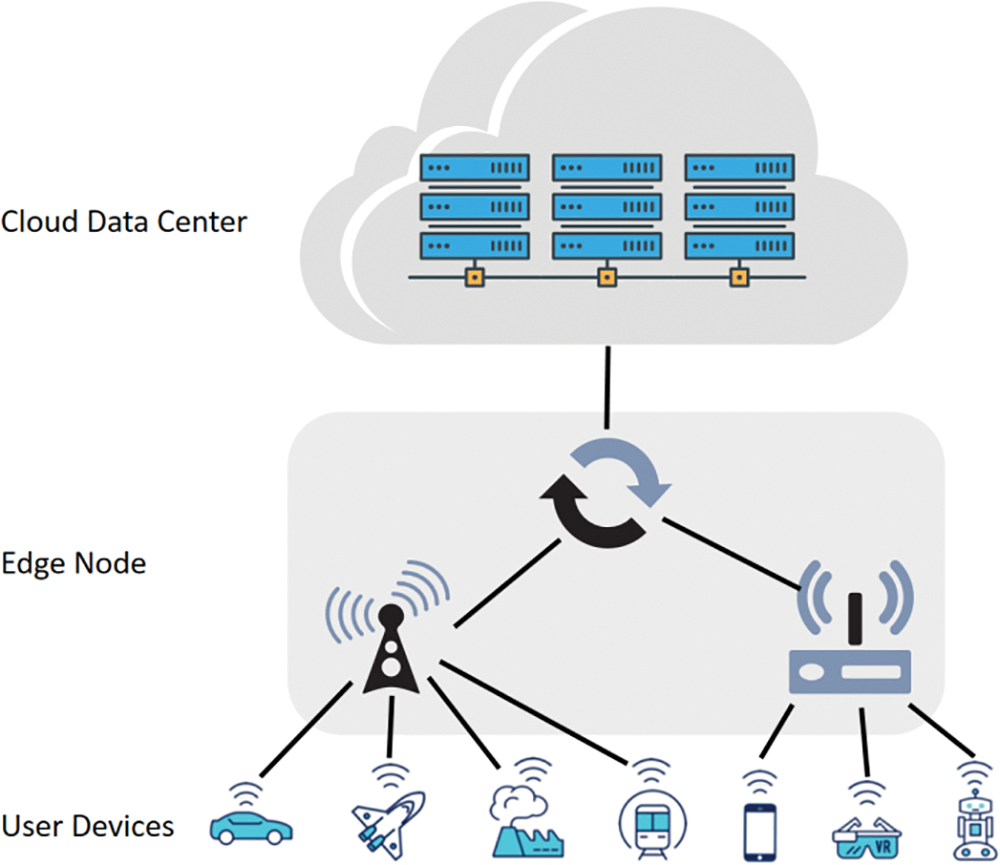
Figure 1: Schematic diagram of an edge computing system consisting of a cloud computing centre, edge devices and user terminals or sensors

Resource allocation refers to how the server manages multiple edge services operating simultaneously, and it is crucial to fully utilize the edge server resources to guarantee the stable quality of service under various network conditions. Resources include radio spectrum resources, CPU, memory, storage space, dedicated computing devices, etc. The resource allocation process aims to maximize resource utilization and models existing tasks as optimization problems [5]. Efficient task scheduling enhances user satisfaction by ensuring the edge server completes user tasks within specified deadlines. Predicting the task execution time is the prerequisite to initiate task scheduling. Based on the predicted execution time and deadline of each task, the edge server enables effective task scheduling and resource allocation to reduce task completion time and improve system performance. The demand for resources, on the other hand, changes dynamically during service operation, and an edge computing device is said to be resource-constrained when the demand for resources for the service it is running exceeds the resources available to the edge computing device. A resource-constrained edge computing device reduces the quality of service (QoS) of the services offloaded to it because it can handle the resource demands of the services. When tasks offloaded to the edge computing device consume more resources than the device's resource limit, it causes the device to be resource-constrained, directly affecting the quality of service (QoS).

To continuously improve user QoE and QoS scientific and reasonable deployment of edge computing device resources become a key element. Numerous research methods have been applied in this field, such as CNN methods [6–8], LSTM methods [9–12], and fuzzy neural network methods [13,14], etc. This paper recommends a novel resource provisioning prediction model for edge computing devices that predicts the load on edge servers. This allows the computing resources (QoS) to be optimized and improved in advance. The model designs a novel network structure that integrates Conv1D, GRU, and LSTM modules for predicting edge server load.

The following are the main contributions of this paper:

(1)   A time series forecasting model incorporating Conv1D, LSTM and GRU is proposed in this study. Conv1D can capture local information while capturing time series dependencies, which improves the capability of the model to extract time series features and improves the accuracy of the proposed model.

(2)   The model can accurately predict the load on edge servers and serve as a foundation for the scientific scheduling of edge device computing resources.

(3)   In this paper, the model was trained and tested using a small dataset collected from small edge devices, achieving competitive results.

The remainder of this article is divided into the following sections: Section 2 briefly summarizes other significant scientific activity on the topic. Section 3 introduces the CLG model's ideas and implementation details. The experimental data and visual analysis are presented in Section 4. The study’s conclusion are outlined in Section 5.

2  Related Work

Machine learning based approaches for edge computing resource scheduling have the following advantages; strong distributed learning and storage capabilities, an associative memory function capable of accurately approximating complex nonlinear relationships, and powerful parallel processing capabilities [6]. The load of the edge computing system is time-series data and hence it is necessary to use time-series data to predict the load. The main deep learning models for temporal data prediction are Conv1D, LSTM, GRU, etc.

Aiming to construct an optimized convolutional neural network (CNN) architecture, Violos et al. [7] proposed a novel hybrid hyperparametric optimization approach that combines particle swarm optimization and Bayesian optimization. This architecture was experimentally validated using an edge computing infrastructure. The evaluation results demonstrate that the proposed regression model performs better in terms of accuracy than other machine learning meta-predictors and resource usage state models. Jia et al. [8] used model compression as an “intra-model” optimization approach and computation sharing as a “inter-model” optimization approach. They proposed a new CNN-based resource optimization approach (CroApp) to improve CNN intra-model performance. Additionally, the method prioritizes resource optimization across applications. According to experiment results, CroApp outperforms existing methods in terms of resource reduction, scalability, and application performance. The Conv1D enables local feature extraction for time series data. The advantage of Conv1D over LSTM and GRU is that the computation speed is faster and the memory consumption is relatively less. In edge device resource prediction, Conv1D may be more suitable than LSTM and GRU if the features of time series data are relatively simple. The disadvantage of Conv1D is its inadequate ability to process long-term dependencies in time series data and its inadequate performance in processing complex time series data.

In order to optimize the dynamic resource allocation for edge computing devices, Selvi et al. [9] used an LSTM neural network to build a network traffic prediction model based on long-term time series of network traffic flow. The experimental results revealed that the model’s prediction accuracy was enhanced. Ashawa et al. [10] established an intuitive dynamic resource allocation system based on the LSTM algorithm for near real-time software simulation to analyze an application’s resource utilization and determine the best additional resources to provide for that application. When compared to other models, the accuracy of this model is improved by about 10%–15%. Yan et al. [11] proposed a Bi-LSTM load prediction algorithm based on an attention mechanism to accurately predict the load of microservices and build a resilient scaling system with automatic scheduling of work nodes. The experimental results show that meeting the SLA of microservices for edge computing improves system resource utilization by about. Lai et al. [12] utilised LSTM to build a non-intrusive load monitoring system, using edge computing to achieve parallel computing and improve the efficiency of device identification, and the random average identification rate could reach 88%. The average identification rate of continuous data of a single electrical device could reach 83.6%, according to the proposed parameter model optimization adjustment strategy. LSTM captures long-term dependencies effectively when processing time-series data. In contrast to traditional RNNs, the internal structure of LSTM contains gate units that are able to selectively remember and forget the input data. This allows LSTM performance in resource prediction for edge computing devices, especially when processing multiple time series features. Nevertheless, the drawbacks of LSTM include high complexity and high computational and memory consumption, making it unsuitable for edge devices with limited resources.

The Bi-LSTM-GRU combined prediction model, proposed by Li et al. [15], effectively combines a Bi-LSTM network with a GRU network for high prediction accuracy and short prediction time. It is validated against several classical time series prediction algorithms on the Google Cloud dataset. The experimental results show that the mean square error (MSE) of the joint Bi-LSTM-GRU prediction model is reduced by about 5%, as is the prediction time. Using a bi-directional long and short-term memory (Bi-LSTM) model and an attention mechanism, Jeong et al. [16] predicted CPU and memory usage. The allocation of resources was adjusted by predicting resource usage to reduce excessive resource usage. Average CPU and memory utilization increased by 23.39% and 42.52%, respectively, over conventional HPA. Furthermore, when compared to conventional HPA, no overload was observed when resources were under-allocated.

Violos et al. [17] proposed a gated recurrent neural network multi-output regression model based on time series resource usage metrics. Edge computing infrastructures are defined by their dynamic and heterogeneous environments. They proposed an innovative Hybrid Bayesian Evolutionary Strategy (HBES) algorithm for automatic adaptation of resource usage models to increase the generality of our approach. In this paper, the proposed mechanism for resource usage prediction has been experimentally evaluated and compared to other state-of-the-art methods, and it shows significant improvements in terms of RMSE and MAE. Lu et al. [18] proposed the IGRU-SD model, which uses an improved GRU neural network integrated with a resource discrete detection module to classify tasks based on resource intensity and predict the expected resource request level, with model prediction accuracy superior to existing ARIMA, RNN, and LSTM prediction models. Catena et al. [19] proposed a distributed prediction technique in which LSTM neural networks exchange only a small number of weights in order to significantly reduce communication overhead compared to the centralized case. They also looked at three different distributed solutions that had lower errors. Wu et al. [20] proposed forecasting the service resource demand based on the resource consumption of cloud platforms and mobile edge computing for the specific scenario of telematics. They also created a multidimensional time series prediction algorithm based on deep learning to create a neural network structure matching business characteristics. The findings show that the method’s prediction accuracy has good application value, laying the groundwork for future research into the mechanism of resource mapping, edge node scheduling, and resource allocation between resource demand and edge stage capability model. The internal structure of GRU is relatively simple, with only two gate units, an update gate and a reset gate. Therefore, GRU has relatively low computation and memory consumption and is suitable for running on edge devices. In addition, GRU is also able to effectively capture the long-term dependencies of time series data and thus performs better in resource prediction for edge devices. Nonetheless, GRU may be slightly worse at processing very long time series data than LSTM.

In this paper, combining the respective advantages of Conv1D, LSTM and GRU, CLG models are constructed to predict the resource occupancy data of edge computing devices from multiple aspects, assisting the edge computing devices to optimize resource provisioning and improve the overall quality of service (QoS) and quality of experience (QoE).

3  Methodology

The CLG model proposed in this paper is trained and tested on a time series dataset. This study combines Conv1D, LSTM and GRU to construct the CLG model, aiming to combine the advantages of different types of networks to improve the prediction accuracy and speed of the model while minimizing the computational effort.

The CLG model predicts the predicted value yi,t of the CPU usage i of the edge computing device at the moment of t, and in general, the predicted value at t + 1 moment can be expressed as

y^i,t+1=f(yi,t−k:t,xi,t−k:t,Si)(1)

where y^i,t+1 is the predicted value from the model, xi,t−k:t={xi,t−k,⋯,xi,t} and yi,t−k:t={yi,t−k,⋯,yi,t} are observations of the target and exogenous inputs over a backward window k, si is static metadata related to CPU usage, and f(⋅) is the prediction function the model learned. Element indices are not included in the following sections unless specifically requested i for the sake of simplicity in representation.

In this paper, the MinMaxScaler method is used to normalize the data and map the data to the interval [0,1], and the MinMaxScaler function equation is as follows:

Xstd=X−X.min(axis=0)X.max(axis=0)−X.min(axis=0)(2)

Xscaled=Xstd∗(max−min)+min(3)

where Xscaled denotes the normalized result, Xstd denotes the normalized result, X.max(axis=0) denotes the row vector consisting of the maximum value of each column in the matrix, X.min(axis=0) denotes the row vector consisting of the minimum value of each column in the matrix, max denotes the maximum value of the interval mapped to 1, and min denotes the minimum value of the interval mapped to 0.

3.1 Conv1D

In the field of deep learning research, CNN is an extremely prevalent network model. Whether in the field of image recognition, computer vision, or speech analysis CNNs demonstrate outstanding performance. In general, CNN is mainly composed of a convolutional layer, pooling layer, and fully connected layer together, usually for processing two-dimensional data such as images. Conv1D [21] (1D Convolutional Neural Network), which is a special structure of CNN, can also apply to the processing of one-dimensional data. Conv1D performs text analysis or time series prediction in simple tasks instead of RNN [22,23] with faster processing speed. The intermediate features of the Conv1D hidden layer, each causal convolutional filter takes the following form:

htl+1=A((W∗h)(l,t))(4)

(W∗h)(l,t)=∑τ=0kW(l,τ)ht−τl(5)

where htl∈ℜℋin is the intermediate state of l layer at the t moment, * is the convolution operation, W(l,τ)∈ℜℋout×ℋin the fixed filter weight of l layer, A(⋅) is the activation function and the relu is used in this paper as the activation function.

The same set of filter weights is used at all times and at each time step in temporal Conv1D, which goes along with the standard Conv1D assumption of spatial invariance. Additionally, Conv1D is limited to producing predictions based on inputs within its predetermined receptive domain or lookback window. To ensure that the model can use all pertinent historical data, the receptive domain size k must be carefully adjusted.

3.2 LSTM

LSTM enhances the capability of RNN networks in processing long-term dependencies, with resistance to gradient vanishing, which is a special kind of recurrent structure [24]. The typical LSTM network cell mechanism is shown in Fig. 2. An LSTM cell consists of a cell, an input gate, an output gate, and a forget gate.

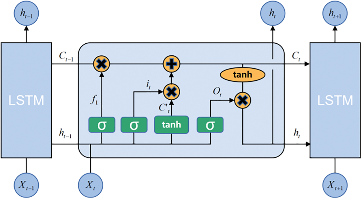
Figure 2: Schematic diagram of LSTM cell

The CELL state is represented by c, the output of the implied state by h, and the activation functions are and tanh in Fig. 2. The input, forget, and output gates are denoted by i, f, and o, respectively.

The input gate i has a value domain of (0, 1), and its main function is to determine the importance of the current input before generating a new memory and, thus to control the size of the newly generated part Ct′ in the CELL state Ct. The input gate structure is shown in Eqs. (6) and (7).

it=σ(wt⋅[ht−1,xt]+bt)(6)

Ct′=tan⁡h(wc⋅[ht−1,xt]+bc)(7)

The function of the forget gate f is to control how much information from the CELL state of the previous moment can be passed to the CELL state of the present moment, filter the information, control the size of the input x and the output h of the previously hidden layer to be forgotten, and determine whether the past memory unit is useful for computing the current memory unit. The goal is to determine whether or not the hidden CELL state of previous layer is forgotten with a certain probability using a value range of (0,1). The equation that follows illustrates the the structure of forget gate:

ft=σ(wf⋅[ht−1,xt]+bf)(8)

The output value of the forget gate f and the input gate i updates the current CELL state in each CELL of the LSTM. As seen in Fig. 2, the new CELL state Ct is divided into two distinct components, the first of which is governed by the previous CELL state Ct−1 and the forget gate f with size (ft×Ct−1). The input gate i, of size (it×Ct′), and the most recent CELL state information Ct′ at this precise moment control the second part. The following equation illustrates the process of updating the CELL state:

Ct=ftiCt−1+itCt′(9)

The role of the output gate o is to separate the final memory from the hidden state and control which information the current neuron needs to output based on the updated CELL state, thus determining the most hidden state final output ht. The output gate structure is shown in the following equation:

ot=σ(wo⋅[ht−1,xt]+bo)(10)

ht=ot×tan⁡h(Ct)(11)

As can be seen from the network structure and formula, each LSTM gate (input gate, forget gate, and output gate) has its own set of parameters (w,b), which is a significant aspect of the LSTM network structure. Similarly, the formula of each hidden neuron, which has the shape of an h, is made up of the current input x and the output of the previously hidden neuron in turn. Because the output of the sigmoid function is (0,1), when the output is close to 0 or 1, in line with the physical sense of off and on, the value of is generally chosen as the excitation function of the sigmoid, which primarily plays the role of gate. Tanh is used as the activation function for the memory cell c, primarily because its output is (−1,1). This is the primary reason why the tanh function was chosen as the memory unit’s activation function, as the gradient converges faster than the sigmoid function near 0. When there is no helpful info within input data, the value of the forget gate f is close to one, and the value of the input gate i is close to zero, saving useful information from the past. When there is valuable information in the input sequence, the forget gate value f is close to 0, and the input gate value is close to 1. The LSTM model will then forget the previous memory and record the relevant information in the present. It can be seen that the three gate structures of the LSTM network, in conjunction with the memory unit, control the network output h, allowing the entire network to effectively control the change of the sequence information.

3.3 GRU

GRU (Gated Recurrent Unit) [25], another improved form of the classical recurrent neural network, is a relatively new network model that, like LSTM, has a strong ability to process time series data while effectively avoiding the gradient vanishing problem.

GRU simplifies some of the gate of LSTM in order to simplify the model and reduce computational costs, and because GRU has more gate than RNN, it achieves the effect of not accepting input from previous neurons. In comparison to the LSTM model, the GRU model combines to “the forget gate” and “input gate” of LSTM into a single “update gate,” with the goal of Fig. 3 depicting the GRU cell structure.

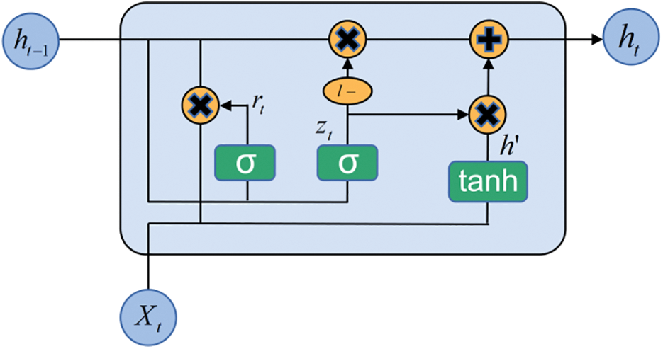
Figure 3: Schematic diagram of GRU cell

Similar to the LSTM model, the GRU model also controls information input and output through “gates”, but the difference is that the GRU is simplified to control information through two gates, called “reset gates” and “update gates”. Using the role of the “gates” as a starting point to derive the GRU forward pass formula, the notation of the formula is as follows:

Γr: the last output of the GRU “reset gate”

Γn: the last output value of the GRU “update gate”

δ: the sigmoid function, which is the activation function of the “gate”

X<t>: the input to the implicit layer at time t

h<t>: the state of the cell at time t

w: the weights of the linear function

b: the bias term of the linear function

To avoid the problem of gradient disappearance and gradient explosion when the RNN sequence is too long, the GRU model is simplified in only two steps. First, the information from the previous CELL is selectively forgotten via the “reset gate” to confirm whether the information passed by the previous CELL is what needs to be remembered. The information from the previous CELL and the information input from the current CELL are combined linearly after the CELL learns the linear weights. The result of this linear combination is then input into the sigmoid function, where it will appear very close to 0 or 1. When the result is close to 0, it indicates that the previous CELL’s information is forgotten, and when it is close to 1, it indicates that the previous CELL’s information is still being remembered. The fundamental formula for this is as follows:

Γr=δ(Wf<t>[X<t>,h<t>]+br<t>)(12)

After the state of the “reset gate” is calculated, this paper then proceeds to the calculation of the candidate activation function value, which is used to combine the information of the previous CELL and this CELL to update the state of the CELL and get the candidate value of the new CELL state, where the value obtained from the “reset gate” tells us how much the correlation between the state of the previous CELL and the state of this CELL.

h^<t>=tan h(Wc<t>[X<t>,Γr∗h<t−1>]+bc<t>)(13)

The role and form of the second “update gate” is similar to that of the “forget gate” in the LSTM in that it determines whether the input information needs to be updated before being passed to the following CELL. The mathematical expression is as follows:

Γn=δ(Wn<t>[X<t>,h<t>]+bn<t>)(14)

After obtaining the states of the two gates and the candidate values for the states, the next step is to combine the information passed in by this CELL with the state passed in by the previous CELL to finalize the state of this CELL, the principle of which is expressed by Eq. (15) as follows:

h<t>=Γn∗h^<t>+(1−Γn)∗h<t−1>(15)

3.4 CLG

Conv1D provides local feature extraction of time series data, with the advantages of fast computation speed and low memory consumption; the disadvantage is the insufficient ability to process the long-term dependency of time series data. LSTM captures long-term dependencies effectively in processing time-series data and enables effective prediction of edge computing device resource usage, especially in cases requiring the processing of multiple time-series features; the drawbacks of LSTM include high model complexity and high computational and memory consumption. Compared with LSTM, GRU may perform slightly worse when dealing with very long time series data but has the advantage of faster computation and relatively less memory consumption. This study combines three models to construct a CLG model for edge computing devices. The model completes the computational resource occupancy prediction assignment with a simpler and lighter structure, supporting the reasonable deployment of edge computing resources. The CLG model structure is shown in Fig. 4.

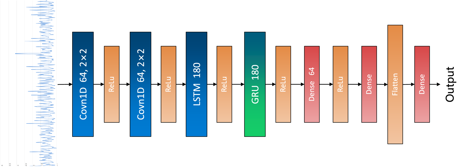
Figure 4: Schematic diagram of the CLG model

Both layers of Conv1D use 64 convolution kernels of size 2 × 2, with the relu as the activation function, to perform cascade convolution on the data; one layer of LSTM uses 180 CELL units to operate on the data, with the relu as the activation function; and one layer of GRU uses 180 CELL units to operate on the data, with the relu as the activation function. Finally, the output of the hybrid model includes two fully connected layers, one Flatten layer, and one more fully connected layer.

4  Experimental

4.1 Experimental Environment

The experimental model was run on the following:

Hardware: WIN10, AMD Ryzen 7 5800X 8-Core@3.8 GHZ + 32G RAM, NIVIDA GeForce GTX 1080 Ti.

Software: Python 3.6.5, PyCharm 2021.3.2 (Community Edition), Keras 2.1.5. Batch size = 64, Optimizer = adam, Loss function = MAPE, Epoche = 400.

4.2 Experimental Data

This study manually intercepts CPU load records of a edge computing device to form a small dataset, totaling 1110 h and 6249 consecutive time points. The small edge computing device is deployed in the middle location of a large residential community, with no universities, shopping malls and other crowded places around it. In the experiments, a training set was formed from sample 1 to sample 5899, and a validation set was formed from sample 5900 to sample 6249. The dataset has been uploaded to https://github.com/AlpacaGlory/A-Novel-Predictive-Model-for-Edge-Computing-Resource-Scheduling-Based-on-Deep-Neural-Network.

4.3 Evaluation Metrics

In this paper, MAE, MSE, RMSE, R2 and training time are used as metrics.

(1) MAE

MAE (Mean Absolute Error), refers to the average of the absolute value of the difference between the predicted value of the model f(x) and the true value of the sample y. The formula is as follows:

MAE=1m∑i=1m|yi−f(xi)|(16)

where f(xi) is the model’s ith predicted value, yi is its ith true value, i∈{1,2,⋯,m} and MAE are in the range [0,+∞), MAE is equal to 0 in the case of an ideal model, where the predicted and true values exactly match. The greater the error, the greater the MAE value.

The MAE is more inclusive and insensitive to outliers as the squared term has no influence. Nevertheless, since the absolute values influence, the MAE provides no indication of whether the model’s predicted value is greater or less than the true value.

(2) MSE

MSE (Mean squared error) refers to the average of the squares of the difference between the model predicted value f (x) and the sample true value y. Its formula is as follows:

MSE=1m∑i=1m(yi−f(xi))2(17)

where f(xi) is the model’s ith predicted value, yi is the model’s ith true value, and i∈{1,2,⋯,m} MSE range [0,+∞), MSE equals 0 when the calculated value exactly matches the true value, i.e., perfect model; the larger the error, the higher the MSE value and the worse the model performance.

The MSE function has a smooth and continuous curve, making gradient descent algorithms easy to derive and use. It is a commonly used loss function. Furthermore, as the error decreases, so does the gradient, facilitating convergence to a minimum value even at a fixed learning rate. MSE, on the other hand, is more sensitive to and affected by outliers.

(3) RMSE

RMSE (Root Mean Square Error) is the square root of MSE, which is used to represent the bias between the predicted value of the model f (x) and the true value of the sample y. Its formula is as follows:

RMSE=1m∑i=1m(yi−f(xi))2(18)

where f(xi) is the ith predicted value of the model, yi is the ith true value, i∈{1,2,⋯,m}. MSE range [0,+∞), RMSE is equal to 0 when the predicted value matches the true value exactly, i.e., perfect model; the larger the error, the larger the MSE value and the worse the model performance.

The RMSE does a square root operation on top of the MSE so that the calculated results are consistent with the predicted and true magnitudes.

(4) R2

R2 (R-squared) One of the common measures of precision used in linear models and analysis of variance, R-squared represents the percentage of variance in a model where the dependent variable can be explained by the independent variable. That is, R2 indicates the level of fit (goodness of fit) of the data to the regression model. The formula for R2 is as follows:

R2=1−SSESST=1−SSESSR+SSE(19)

where SSR is the sum of squared regressions, SSE is the sum of squared residuals and SST is the sum of squared total deviations, with the following equations:

SSR=∑i=1m(f(xi)−y¯)2(20)

SSE=∑i=1m(yi−f(xi))2(21)

SST=SSR+SSE=∑i=1m(yi−y¯)2(22)

thenR2=1−∑i=1m(yi−f(xi))2∑i=1m(yi−y¯)2(23)

where f(xi) is the ith predicted value of the model, yi is the ith true value, i∈{1,2,⋯,m}, and y¯ is the mean of the true values. R2 ranges between [0,1], and the closer to 1, the better. The indicator used to measure the best linear regression is R2, which usually indicates a good or bad model fit.

4.4 Comparative Experiments

In this study, the CLG model was compared with Conv1D [21], RNN [26], BiLSTM [27], and logistic regression [28] algorithms. The comparison includes evaluation metrics, training time. Table 1 shows the results of experiments comparing CLG with different algorithms.

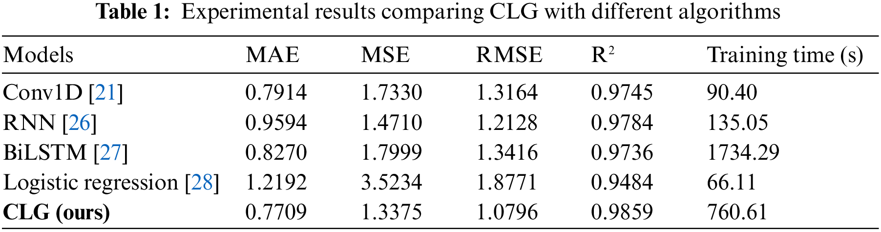
As shown in Table 1, there is a significant difference in the evaluation metrics between the CLG model and the other algorithms, showing that the CLG model has higher prediction accuracy, reflecting its intentional performance. R2 shows that the lowest score among the models is 97.36%, while the highest score reaches 98.59%, indicating that all four models perform well. In terms of the MAE metric, the RNN model has the largest value, indicating that the model has a relatively large error, while the CLG model has the smallest value, indicating that the model has the smallest error. In terms of MSE, the smaller values for the CLG and RNN models indicate that the prediction errors of these two models are small and concentrated, while the larger values for the Conv1D and BiLSTM models indicate that the prediction errors are relatively scattered [29–31]. In terms of R2 metrics, the higher values for the CLG and RNN models showed that such models’ prediction performance is strong. The prediction results are in good agreement with the actual situation. In contrast, the slightly lower values for the Conv1D and BiLSTM models demonstrate that the model’s prediction accuracy is also high but slightly lower than the other two models. In terms of training time, the Conv1D and RNN models have the shortest time, which is due to the simplicity of these two models and the small size of the network, which makes them faster. The experimental results show that for the self-built dataset of this study, the logistic regression algorithm has slightly lower prediction results than other network models. The reason for this is probably that logistic regression is a linear classification model that can effectively process linearly differentiable data. Whereas the self-built dataset in this study is time series data with no direct logistic relationship, which means that the data itself is nonlinear, and therefore, the performance of logistic regression is lower than that of other network models. The CLG model synthesizes the advantages of Conv1D, LSTM and GRU, which can extract time series data features in multiple scales and more accurately predict the CPU occupancy of edge servers, showing competitive performance.

Fig. 5 shows the predicted CPU load vs. the actual load curve for each model. It can be seen that all four models make accurate judgments about the trend of load changes, and the prediction curves reflect each gradient change of the real curve, but the different models show different degrees of prediction. In the data set used in this study, the data content is simple and the data features are not difficult to extract, so good prediction results can be obtained for simple network structures [32,33]. The most volatile of the four models is the Conv1D model, which has a good overall fit as indicated by the evaluation metrics, but some of the predicted values are too far off. The CLG model is the closest to the true value, with only small fluctuations in some of the predicted values, proving that the model fits well.

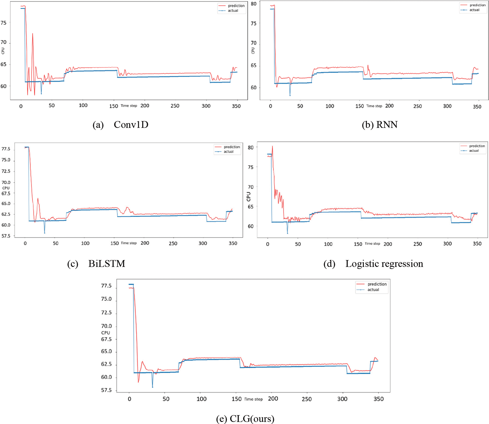
Figure 5: The comparison between predicted and actual load for CPU

The loss function curves for each model are shown in Fig. 6. As recurrent network models, RNN and BiLSTM models have only one layer due to their extremely simple structures, they show relatively large fluctuations in both the training process and the testing process, while the Conv1D model has relatively less fluctuations in both the training and testing processes, but there is a gap between the training and testing processes. The CLG model has a relatively high fit in both the training and testing processes, reflecting good. The CLG model has good stability and shows good generalization ability of the model.

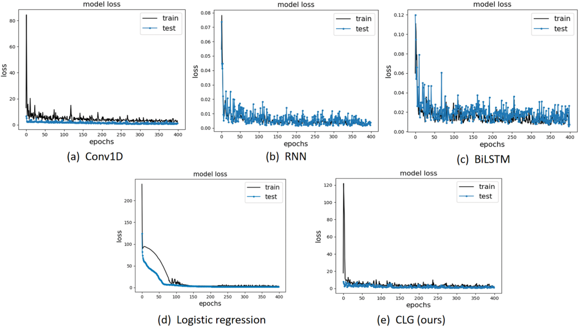
Figure 6: Evolution of training and testing losses for different models

4.5 Ablation Experiments

To verify the validity of the model, ablation experiments were conducted. C represents the Covn1D, L represents the LSTM, and G represents the GRU.

(1) C+L

As shown in Table 2, when GRU is not used, the MSE indicator error of the model increases, reflecting the widening of the fluctuation range of the predicted values of the model and the decrease in the stability of the prediction. The change in the MSE indicator is confirmed by the prediction curve in Fig. 7, which also shows a small shift in the prediction curve. In spite of this, the overall predictive ability of the model is still good. This suggests that the presence of the GRU improves the predictive stability of the model. On the other hand, the training time of the model is reduced to about 465 s, suggesting that the GRU significantly impacts the computation speed.

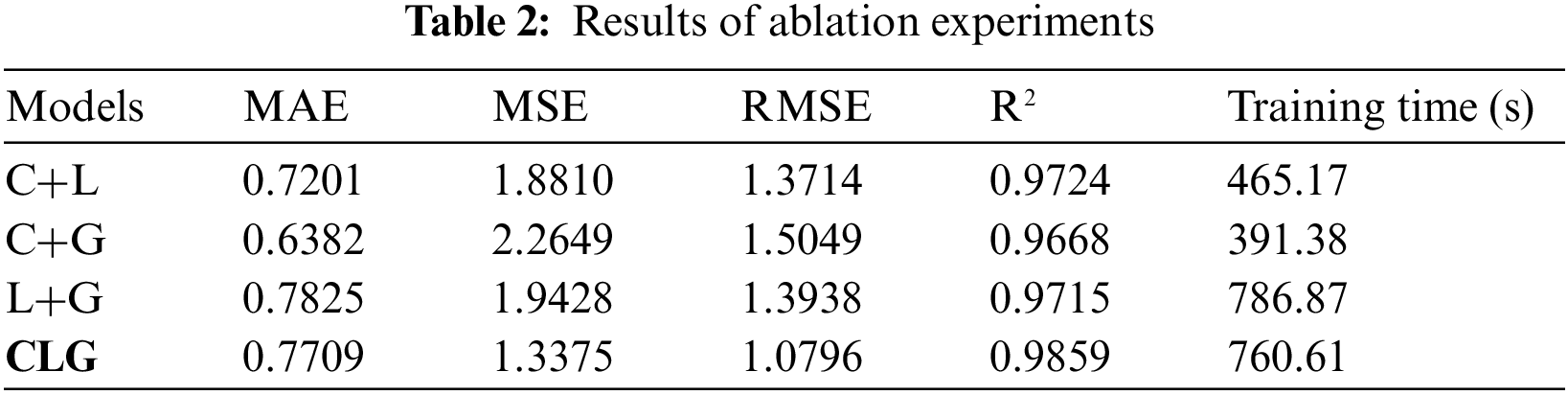
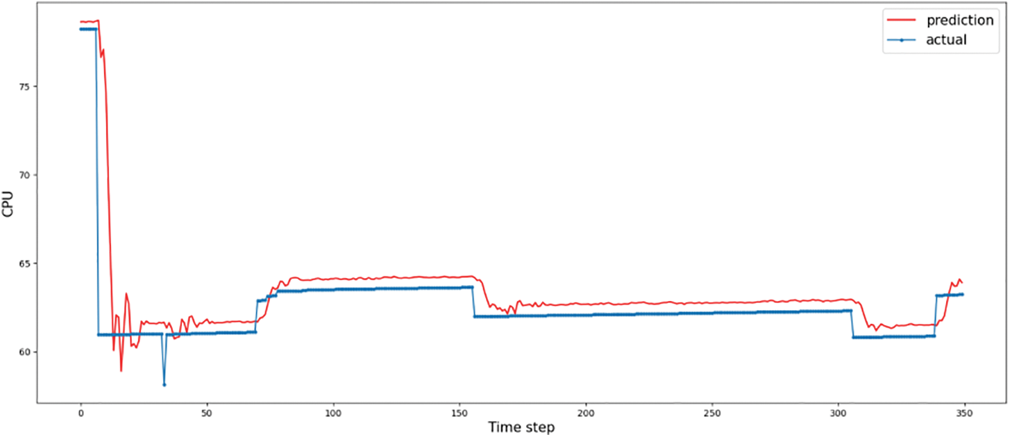
Figure 7: The comparison between predicted and actual load using C+L for CPU

(2) C+G

As shown in Table 2, when LSTM is not used, the MSE indicator error of the model increases, reflecting the widening of the fluctuation range of predicted values of the model. As shown in Fig. 8, the prediction curve changes dramatically, with sharp fluctuations in predicted values, in line with the MSE indicator. The C+G prediction curve fits the true value curve better than the C+L curve. The functions of the LSTM include improving the stability of the model. In terms of training time, the model was further reduced to around 391 s, suggesting that the GRU is less computationally intensive than the LSTM, which is consistent with the relationship between the two, as the GRU simplifies the actual LSTM.

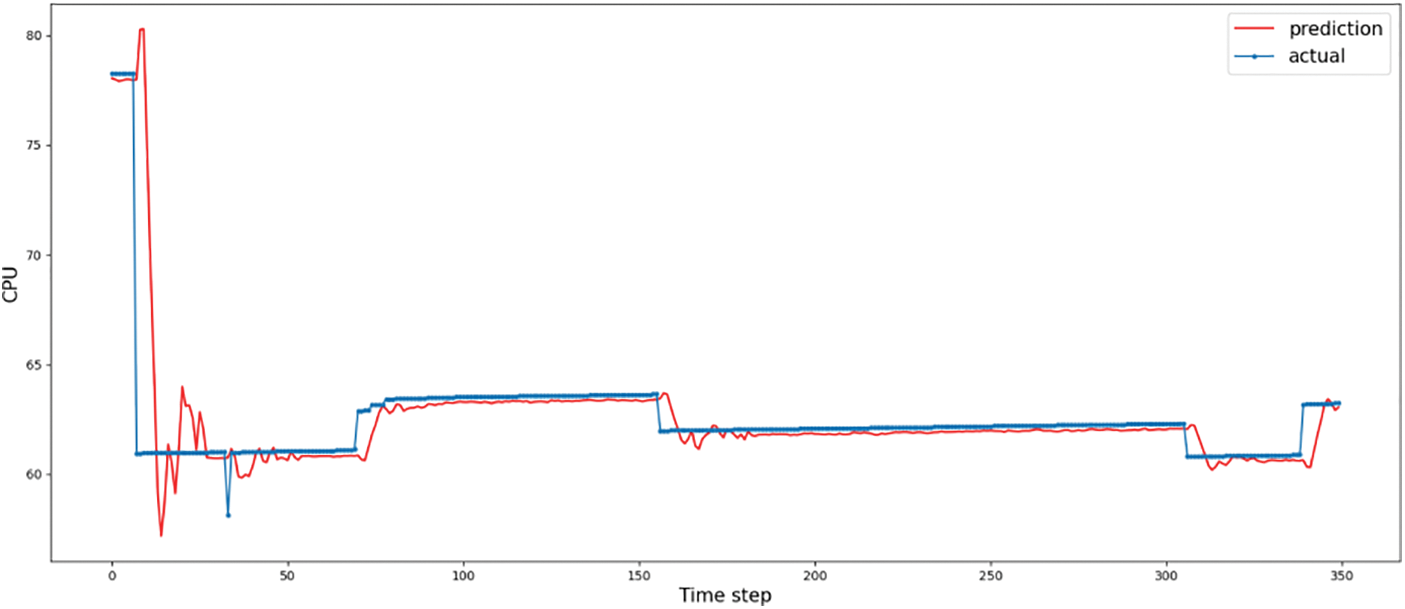
Figure 8: The comparison between predicted and actual load using C+G for CPU

(3) L+G

As shown in Table 2, when Conv1D is not used, the MSE indicator error of the model increases, reflecting the widening of the range of fluctuations in the predicted values of the model. As shown in Fig. 9, combined with the change in the prediction curve, the change in the magnitude of the curve fluctuation can be seen clearly, while the curve shows a drift, which affects the prediction accuracy. The presence of the Conv1D suggests that the prediction curve can be better fitted to the true curve, improving the accuracy of the prediction model. In terms of training time, it increased significantly to about 786 s, even more than the CLG model as a whole, indicating that the existence of Conv1D can reduce the computational workload and shorten the training time, and also indicating that the LSTM and GRU are the most computationally intensive parts of the model.

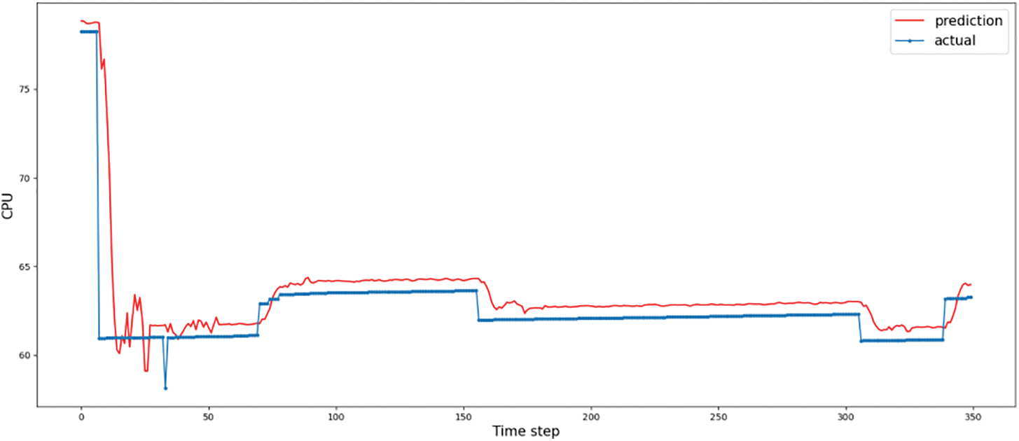
Figure 9: The comparison between predicted and actual load using L+G for CPU

5  Conclusion

In this paper, a CLG model for predicting the load of edge servers is proposed, which provides a scientific basis for scientific scheduling of computing resources of edge devices. After a series of experiments, the following conclusions are drawn. (1) Conv1D can efficiently acquire local features of time series data; (2) LSTM can obtain the global features of time series data and establish the temporal connection between the features, but the model parameters are relatively complex and have a significant impact on the length of the model training time; (3) GRU obtains global features of time series data, but its relatively simple structure can alleviate the problem of gradient disappearance and improve the robustness of the model; (4) Experimentally verified that the CLG model can acquire multi-scale time series data features and has good robustness, it is an accurate and efficient CPU load prediction model for edge computing devices, and provides an effective method for scientific deployment of edge computing device resources.

Acknowledgement: We thank the editor and anonymous reviewers for their valuable comments.

Funding Statement: This work was supported in part by the National Natural Science Foundation of China under Grant 62172192, U20A20228, and 62171203, in part by the Science and Technology Demonstration Project of Social Development of Jiangsu Province under Grant BE2019631.

Author Contributions: The authors confirm contribution to the paper as follows: study conception and design: Pengjiang Qian, Wenjun Hu; data collection: Jian Yao; analysis and interpretation of results: Ming Gao, Weiwei Cai, Yizhang Jiang; draft manuscript preparation: Ming Gao, Weiwei Cai. All authors reviewed the results and approved the final version of the manuscript.

Availability of Data and Materials: The dataset used to support the findings of this study has been uploaded to https://github.com/AlpacaGlory/A-Novel-Predictive-Model-for-Edge-Computing-Resource-Scheduling-Based-on-Deep-Neural-Network.

Conflicts of Interest: The authors declare that there is no conflict of interest regarding the publication of this paper.

References

1. Jararweh, Y., Doulat, A., AlQudah, O., Ahmed, E., Al-Ayyoub, M. et al. (2016). The future of mobile cloud computing: Integrating cloudlets and mobile edge computing. 2016 23rd International Conference on Telecommunications (ICT), pp. 1–5. Thessaloniki, Greece, IEEE. https://doi.org/10.1109/ICT.2016.7500486 [Google Scholar] [CrossRef]

2. Khayyat, M., Alshahrani, A., Alharbi, S., Elgendy, I., Paramonov, A. et al. (2020). Multilevel service-provisioning-based autonomous vehicle applications. Sustainability, 12(6), 1–16. [Google Scholar]

3. Mach, P., Becvar, Z. (2017). Mobile edge computing: A survey on architecture and computation offloading. IEEE Communications Surveys & Tutorials, 19(3), 1628–1656. [Google Scholar]

4. Hong, C. H., Varghese, B. (2019). Resource management in fog/edge computing: A survey on architectures, infrastructure, and algorithms. ACM Computing Surveys (CSUR), 52(5), 1–37. [Google Scholar]

5. Zhao, Z. W. (2021). Principles, technologies and practices of edge computing, vol. 29. First edition. Beijing, China: Machinery Industry Press. [Google Scholar]

6. Luo, Q., Hu, S., Li, C., Li, G., Shi, W. (2021). Resource scheduling in edge computing: A survey. IEEE Communications Surveys & Tutorials, 23(4), 2131–2165. [Google Scholar]

7. Violos, J., Pagoulatou, T., Tsanakas, S., Tserpes, K., Varvarigou, T. (2021). Predicting resource usage in edge computing infrastructures with CNN and a hybrid Bayesian particle swarm hyper-parameter optimization model. Intelligent Computing: Proceedings of the 2021 Computing Conference, vol. 2, pp. 562–580. Saga, Japan, Springer International Publishing. [Google Scholar]

8. Jia, Y., Liu, B., Dou, W., Xu, X., Zhou, X. et al. (2022). CroApp: A CNN-based resource optimization approach in edge computing environment. IEEE Transactions on Industrial Informatics, 18(9), 6300–6307. [Google Scholar]

9. Selvi, K. T., Thamilselvan, R. (2021). Dynamic resource allocation for SDN and edge computing based 5G network. 2021 Third International Conference on Intelligent Communication Technologies and Virtual Mobile Networks (ICICV), pp. 19–22. Tirunelveli, India, IEEE. https://doi.org/10.1109/ICICV50876.2021.9388468 [Google Scholar] [CrossRef]

10. Ashawa, M., Douglas, O., Osamor, J., Jackie, R. (2022). Improving cloud efficiency through optimized resource allocation technique for load balancing using LSTM machine learning algorithm. Journal of Cloud Computing, 11(1), 1–17. [Google Scholar]

11. Yan, M., Liang, X., Lu, Z., Wu, J., Zhang, W. (2021). HANSEL: Adaptive horizontal scaling of microservices using Bi-LSTM. Applied Soft Computing, 105(7), 107216. [Google Scholar]

12. Lai, C. F., Chien, W. C., Yang, L. T., Qiang, W. (2019). LSTM and edge computing for big data feature recognition of industrial electrical equipment. IEEE Transactions on Industrial Informatics, 15(4), 2469–2477. [Google Scholar]

13. Li, F., Zheng, T., Cao, Q. (2023). Modeling and identification for practical nonlinear process using neural fuzzy network-based Hammerstein system. Transactions of the Institute of Measurement and Control, 45(11), 2091–2102. [Google Scholar]

14. Li, F., Zhu, X., Cao, Q. (2023). Parameter learning for the nonlinear system described by a class of Hammerstein models. Circuits, Systems, and Signal Processing, 42(5), 2635–2653. [Google Scholar]

15. Li, X., Wang, H., Xiu, P., Zhou, X., Meng, F. et al. (2022). Resource usage prediction based on BiLSTM-GRU combination model. 2022 IEEE International Conference on Joint Cloud Computing (JCC), pp. 9–16. Fremont, CA, USA, IEEE. https://doi.org/10.1109/JCC56315.2022.00009 [Google Scholar] [CrossRef]

16. Jeong, B., Baek, S., Park, S., Jeon, J., Jeong, Y. S. (2023). Stable and efficient resource management using deep neural network on cloud computing. Neurocomputing, 521, 99–112. [Google Scholar]

17. Violos, J., Tsanakas, S., Theodoropoulos, T., Leivadeas, A., Tserpes, K. et al. (2021). Hypertuning GRU neural networks for edge resource usage prediction. 2021 IEEE Symposium on Computers and Communications (ISCC), pp. 1–8. Athens, Greece, IEEE. https://doi.org/10.1109/ISCC53001.2021.9631548 [Google Scholar] [CrossRef]

18. Lu, Y., Liu, L., Panneerselvam, J., Yuan, B., Gu, J. et al. (2019). A GRU-based prediction framework for intelligent resource management at cloud data centers in the age of 5G. IEEE Transactions on Cognitive Communications and Networking, 6(2), 486–498. [Google Scholar]

19. Catena, T., Eramo, V., Panella, M., Rosato, A. (2022). Distributed LSTM-based cloud resource allocation in network function virtualization architectures. Computer Networks, 213(3), 109111. [Google Scholar]

20. Wu, M., Rui, L., Chen, S., Yang, Y., Qiu, X. et al. (2022). Design and simulation of resource demand forecasting algorithm in vehicular edge network. Proceedings of the 11th International Conference on Computer Engineering and Networks, pp. 1559–1568. Singapore, Springer. [Google Scholar]

21. Kiranyaz, S., Ince, T., Gabbouj, M. (2015). Real-time patient-specific ECG classification by 1-D convolutional neural networks. IEEE Transactions on Biomedical Engineering, 63(3), 664–675. [Google Scholar] [PubMed]

22. Nguyen, C., Klein, C., Elmroth, E. (2019). Multivariate LSTM-based location-aware workload prediction for edge data centers. 2019 19th IEEE/ACM International Symposium on Cluster, Cloud and Grid Computing (CCGRID), pp. 341–350. Larnaca, Cyprus, IEEE. https://doi.org/10.1109/CCGRID.2019.00048 [Google Scholar] [CrossRef]

23. Zaman, S. K. U., Jehangiri, A. I., Maqsood, T., Umar, A. I., Khan, M. A. et al. (2022). COME-UP: Computation offloading in mobile edge computing with LSTM based user direction prediction. Applied Sciences, 12(7), 3312. [Google Scholar]

24. Hochreiter, S., Schmidhuber, J. (1997). Long short-term memory. Neural Computation, 9(8), 1735–1780. [Google Scholar] [PubMed]

25. Cho, K., van Merriënboer, B., Gulcehre, C., Bahdanau, D., Bougares, F. et al. (2014). Learning phrase representations using RNN encoder-decoder for statistical machine translation. arXiv preprint arXiv:1406.1078. [Google Scholar]

26. Williams, R. J., Zipser, D. (1989). A learning algorithm for continually running fully recurrent neural networks. Neural Computation, 1(2), 270–280. [Google Scholar]

27. Yildirim, Ö. (2018). A novel wavelet sequence based on deep bidirectional LSTM network model for ECG signal classification. Computers in Biology and Medicine, 96, 189–202. [Google Scholar] [PubMed]

28. Hosmer Jr, D. W., Lemeshow, S., Sturdivant, R. X. (2013). Applied logistic regression, vol. 398. Hoboken, New Jersey, USA, John Wiley & Sons. [Google Scholar]

29. Eramo, V., Catena, T. (2022). Application of an innovative convolutional/LSTM neural network for computing resource allocation in NFV network architectures. IEEE Transactions on Network and Service Management, 19(3), 2929–2943. [Google Scholar]

30. Chen, L., Zhang, W., Ye, H. (2022). Accurate workload prediction for edge data centers: Savitzky-Golay filter, CNN and BiLSTM with attention mechanism. Applied Intelligence, 52(11), 13027–13042. [Google Scholar]

31. Zhang, Y., Liu, Y., Guo, X., Liu, Z., Zhang, X. et al. (2022). A BiLSTM-based DDoS attack detection method for edge computing. Energies, 15(21), 7882. [Google Scholar]

32. Gopalakrishnan, T., Ruby, D., Al-Turjman, F., Gupta, D., Pustokhina, I. V. et al. (2020). Deep learning enabled data offloading with cyber attack detection model in mobile edge computing systems. IEEE Access, 8, 185938–185949. [Google Scholar]

33. Vijayasekaran, G., Duraipandian, M. (2022). An efficient clustering and deep learning based resource scheduling for edge computing to integrate cloud-IoT. Wireless Personal Communications, 124(3), 2029–2044. [Google Scholar]