Fuzzy Difference Equations in Diagnoses of Glaucoma from Retinal Images Using Deep Learning

1  Introduction

Glaucoma occurs due to damage to the nerve that connects the eye to the brain, known as the optic nerve. Glaucoma is one of the silent disorders that human beings can get without previous physical signs or symptoms. Tjandrasa et al. [1] assumed that individuals with glaucoma could lose their optic nerve tissues which could lead to losing their vision. Unfortunately, there is no cure for a glaucomatous eye. With that being said, early discovery of the glaucomatous eye can slow down the damage to the optic nerve which can fortunately save the affected individual’s vision. The Cup to Disk Ratio (CDR) is the primary tool used to check whether the individual is at hazard for glaucoma or not. The CDR and ISNT (inferior (I) > superior (S) > nasal (N) > temporal (T)) are the two key diagnostic tools used to evaluate the Optic Nerve Head (ONH). The CDR is a rule that was developed through manual estimation by an ophthalmologist. Despite its benefits, manually monitoring ONH adjustment is a time-consuming process. Since the early diagnosis of this disease is necessary to prevent vision loss, numerous efforts have been made to the programmed discovery of glaucoma at an early stage. Apart from this, optimized medical-aided diagnosis and treatment were analyzed by Zhang et al. [2].

This paper is structured as follows Section 2 provides a literature review of what has been previously done in this field of research. Section 3 discusses the concepts of intuitive fuzzy sets. Section 4 outlines the approach used in retinal image enhancement using fuzzy concepts and the implementation through CNN. This section also analyzes fuzzy manipulation and defuzzification techniques related to CDR. Section 5 deals with fuzzy image segmentation which is used to integrate all the detected regions and partition the image based on similar and dissimilar concentration levels. Spatial frequency fuzzy metric concepts are also discussed for generating a threshold image. In Section 6, numerical illustrations and the various results that were obtained are analyzed.

2  Literature Review

Haubecker et al. [3] proposed a neuro-fuzzy inference system to detect glaucoma using higher-order spectra (HOS) and discrete wavelet transform (DWT) which was based on the criterion of diffuse expulsion. The proposed system was tested on a series of actual ophthalmic images of normal and glaucomatous cases. The most important parameters were then extracted, after having recognized the elliptical form of both the optic disc and boundary. After extracting the highlights, a factual analysis was performed on the partitioned separation. Finally, Dehghani et al. [4] proposed an assortment of algorithmic rules based on fuzzy logic approaches to determine the condition of the patient’s eye. The condition of the eye was then distinguished into three categories including normal, mild glaucoma, and direct/severe glaucoma. Naik et al. suggested a fuzzy set theory-based image enhancement method on HSV (hue, saturation, value) images by applying Gaussian distribution on S and V parameters [5].

The optic disc cup and the parameters of the optic plate were used in the assessment of the glaucoma clutter. Fard et al. [6] utilized a Support Vector Machine (SVM) when calculating the F-cut done through the use of random mass transformation. Among the various detection techniques, background image-based detection of the retina plays an important role as it was subjected to non-invasive detection methods. Then, they made the categorization after selecting the shape. Detecting glaucoma disorder could be achieved by determining the shape of the retina and checking various medical characteristics of the eyes, such as measurements of the thickness of the retinal nerve fiber layer, the relationship between the edge and the disc, the optic disc and the head of the nerve. Rahman et al. [7] investigated the distinct techniques of glaucoma detection using retinal base images. Sharma et al. [8] studied retinal blood vessel segmentation like glaucomatous eye image segmentation.

Soltani et al. [9] predicted glaucoma in the early stage by identifying several characteristics of glaucoma which could be represented as (i) open-tangent glaucoma, (ii) closed-angle Glaucoma, (iii) normal-tension glaucoma, and (iv) connective glaucoma. Welfer et al. [10] tested tonometry (measures the pressure within the eye), ophthalmoscopy (inside the fundus of the eye and other structures), perimetry (systematic calculation of the visual field), gonioscopy (anatomical angle developed between the eye’s cornea and iris) and pachymetry (measures the thickness of the eye’s cornea) and noted that these tests need to be conducted to detect glaucoma. Recently, the detection of glaucoma has been achieved using Random-Forest classifiers with a 91% accuracy. Blurred convergence of inbreeding glaucoma was used to locate the optical resolution in the retinal frame. A test for glaucoma was performed using a digital eye camera to check for optical coherence tomography (OCT), measurement of intraocular pressure (IOP), and evaluations of optic nerve hypoplasia (ONH), retinal nerve fiber layer (RNFL), and visual field defects [11].

The SVM is a supervised machine learning algorithm that can be used for both classification and regression challenges which can be utilized in the process of glaucoma detection [12]. This method is based on the adaptive threshold and it improves the image quality by removing the noises in the image. On retinal images, Li et al. [13,14] and Vostatek et al. [15] proposed vessel segmentation and amplitude estimation utilizing large-scale production of matching filtered responses.

Gour et al. [16] reported an approach to detect the order of glaucoma using eye-based images. This was done through a computerized diagnostic system that was used to find the malformation present in the fundus images. Fraz et al. [17] developed the method of perceiving glaucoma progression using Heidelberg Retinal Tomography (HRT) images. Fuzzy differential equations (FDE) along with intuitionistic fuzzy sets (IFS) are used to develop reliable traffic management systems and shift scheduling for supporting an automatic transmission along with artificial intelligence (AI). In robotics, FDE brings changes in the navigational directions to avoid the obstacle. Furthermore, it can be used in finding the difference between the crossover rate and mutation rate in the genetic algorithmic optimization process.

3  Intuitive Fuzzy Set (IFS)

For a fixed set X1, the fuzzy set of A1 is defined as

A1={<x,μX1(x)>|x∈X1}

μA1 (x): X1→[0,1] defines the minimum and maximum degrees of the element x∈X1 to the set A1. For a fixed set X1, an IFS of A1 is an optimal identifier and it is classified as

A1={<x,μA1(x),vA1(x)>|x∈X1}

Here μA1 (x): X1→ [0, 1] and vA1 (x): X1→[0,1] defines the membership function degrees and the degrees of specific n-membership function whose element x∈X1 to the set A1. This IFS is used to identify the max-min-max of membership and non-membership functions and this leads to classifying the differences between the input values or functions. For every x∈X1, 0 ≤  μA1 (x) + vA1 (x) ≤ 1 and the quantity πA1(x) =  1−μA1 (x) − vA1 (x) is called the intuitive index or index of hesitation, which may require membership value, non-membership value, or both. Note that fuzzy sets are intuitive fuzzy sets (IFS), but the opposite is not necessarily true. Furthermore, A1 is an IFS of the set X1 and that R1 is a conditional relation of X1→Y1, then the composition B1 max-min-max of IFS X1 with the IF relation R1(X1→Y1) is defined as B1=R1,  A1 with membership and non-membership functions defined in Eqs. (1) and (2), respectively:

μB1(y)=maxx∈X1⁡{min [ μA1(x) , μR1(x, y)]}(1)

nB1(y)=minx∈X1⁡{max [ vA1(x) , vR1(x, y)]}(2)

Here, Eqs. (1) and (2) are used to identify the max-min (μB1(y)) and min-max (nB1(y)) values of membership and non-membership functions. The difference between max-min and min-max was measured through the fuzzy difference equation by Alamin et al. [18]. The relationship between symptoms and disease is classified in the following manner:

S1={s1,s2,…,sm}

D1={d1,d2,…,dn}

P1={p1,p2,…,pq}

where S, D, and P are the finite sets of symptoms, type of disease, and patients, respectively. Fuzzy Relations (FR) are defined as Q1 and R1 in Eqs. (3) and (4), respectively:

Q1={<(p,s), μQ1(p,s),vQ1(p,s)>|(p,s)∈P1×S1}(3)

R1={<(s,d), μR1(s,d),vR1(s,d)>|(s,d)∈S1×D1}(4)

where μQ1(p,s) indicates the degree to which symptoms appear inpatient p and vQ1(p,s) indicates the degree to which symptoms do not appear inpatient p. Similarly, μR1(s,d) indicates the degree to which symptoms confirm disease d and vR1(s,d) indicates the degree to which symptoms do not confirm disease d. Composition T1 of the IFR’s R1 and Q1(T1=R1Q1) describes the patient’s pi status in terms of P1 to D1. Glaucoma diagnosis was accomplished by utilizing a Convolutional Neural Network (CNN) which was used to classify glaucomatous and non-glaucomatous cases and this classification was made by the fuzzy difference Eq. (19). The proposed algorithm took an eye image as its input and assigned the values of membership function to relate its weights and biases using optimization function through deep learning [19]. Then, the CNN carefully separated and differentiated the eye images from one another [20]. This included for example differentiating an image with early stage of a glaucomatous eye from a glaucomatous eye where the case is more severe. This helped to enter deeply as

μT1(pi, d)=maxs∈S1⁡{min [ μQ1(pi, d) , μR1(s, d)]}(5)

vT1(pi, d)=mins∈S1⁡{max [ vQ1(pi, d) , vR1(s, d)]}   ∀ pi∈P1and d∈D1(6)

Based on the max–min consensus convergence algorithm, each stage was iteratively updated according to its weighted average together with its minimum and maximum stages from early stage to glaucomatous eyes [21].

From Q1 to R1, a new IFR T1 measurement could be calculated for which, in general, the patient’s diagnosis was labelled p for any type of disease d, to satisfy the following:

  (i)  ST1=μT1−vT1⋅πT1is greatest and(7)

  (ii)  The equality T1=R1∘Q1is retained.(8)

It was also applied to the three aforementioned categories, including glaucomatous, suspected to be glaucomatous, and non-glaucomatous [22]. This new measure T1 interprets the highest levels of association and the lowest degree of non-association of symptoms, as well as the lowest levels of the intuitionistic index in diagnoses. If almost equal values are obtained for a different diagnosis in T1, in this case, the minimal intuitionistic index is considered [23].

3.1 Image Enhancement Using Fuzzy

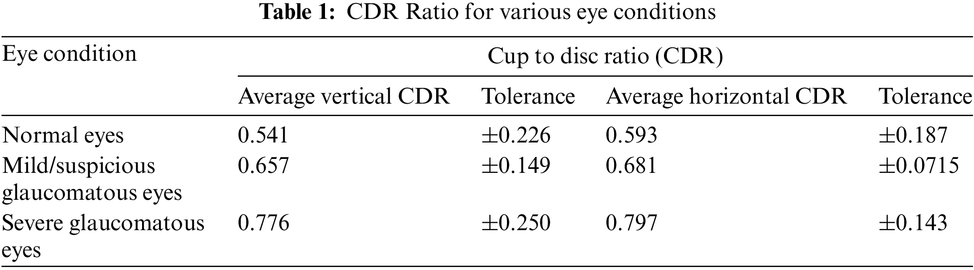
Some numerical specifications were required to enhance the image. Here, we considered the main CDR, optic nerve head, and area of optic nerve values. In general, CDR ranged from 0.26 to 0.5 mm. The average optic nerve head diameter varied from 1.2 to 2.5 mm. The area of the optic nerve head in mm2 was calculated using Eq. (6):

AONH=πr4 ×horizontal diameter (mm)×vertical diameter (mm)(9)

The predicted retinal image’s cup to disc values for average vertical CDR ranged from 0.541 (±0.226) to 0.593 (±0.187) for average horizontal CDR. The retinal image’s cup to disc values for suspected glaucoma ranged from 0.657 (±0.149) for vertical CDR to 0.681 (±0.0715) for horizontal CDR. For glaucomatous eyes, the vertical CDR range was 0.776 (±0.250), and the horizontal CDR was 0.797 (±0.143) as shown in Table 1.

Let us consider a retinal image I1 of dimension M1×N1 (used to calculate CDR value) and intensity range from 0 to L1− 1, defined as

I1=Ui=1M1Uj=1N1μij(x)xmax−xmin(10)

where μij(x) denotes the degrees of the membership function, with the dimension M1×N1 of image I1. The membership function μI1(x) for image I1 could be determined as

μij(x)=xij−xminxmax−xmin(11)

where xij∈I1. xmax is the maximum intensity of the horizontal view of the retinal image I1⋅xmin is the minimum intensity of the vertical view of retinal image I1.

3.2 Fuzzy Difference Equation Computation to Detect Glaucoma in Retinal Images

The first step for fuzzy computation of the retinal image I1 is to break the set of normalized concentration levels which was calculated using Eq. (10) into three fuzzy partition sets {I01,I11,I21} as normal eyes, suspicious (may have glaucomatous) eyes, and glaucomatous eyes, respectively. The partitioned sets of membership functions were represented as μI01, μI11, and μI21, were defined using Eq. (11), and expressed through FDE as follows:

μI01(x)=(1−μij(x))22,∀μ(x)∈I01(12)

μI11(x)=(1−μij(x))22,∀μ(x)∈I11(13)

μI21(x)=(1−μij(x))22,∀μ(x)∈I21(14)

The membership degrees of the three fuzzy sets (three images to be analyzed) described by using Eqs. (12)–(14) must be added and equated with one in accordance with the partition definition. Consequently, the fuzzy degrees of belonging together with the weighted values ωIp1(x) of the concentration level between the series of fuzzy partitions of the concentration levels Ip1(x) must satisfy the following three-layered deep learning condition:

ωI11(x)+ωI21(x)+ωI31(x)=1, ∀μ(x)∈I1

Then, an instruction parameter θ∈[0, 1] was considered to calculate the fuzzy weighted regularization between the images. The three sets (layers) of calibrated weighted fuzzy partitions utilized a deep learning optimized function and the attenuation parameter θ∈[0, 1] was represented as follows:

ωIp1(x)=(μIp1(x)∑μIp1(x))θ, ∀μ(x)∈Ip1(15)

The fuzzy degrees of belonging, together with the weighted values ωIp2(x) whose concentration level between the series of fuzzy partitions of concentration levels Ip2(x) and p2, must satisfy the following conditions:

ωI11(x)+ωI21(x)+ωI31(x)=1, ∀μ(x)∈I2(16)

Now, the fuzzy weighted regularization could be calculated for the second image using the attenuation parameter θ∈[0, 1]:

ωIp2(x)=(μIp2(x)∑μIp2(x))θ, ∀μ(x)∈Ip2(17)

Similarly, the fuzzy degrees of belonging together, along with the weighted values ωIp3(x) of the concentration level between the series of fuzzy partitions of the concentration levels Ip3(x) for p3, must satisfy the following condition:

ωI11(x)+ωI21(x)+ωI31(x)=1, ∀μ(x)∈I3(18)

The three sets of calibrated weighted fuzzy partitions that use the attenuation parameter θ∈[0, 1] are represented as follows:

ωIp3(x)=(μIp3(x)∑μIp3(x))θ, ∀μ(x)∈Ip3(19)

After changing the membership degree, the membership gradation for the sets μIp(x), p= {0, 1, 2} could be estimated. Rearranging for μIp1 from Eq. (14):

μIp1(x)=∏p1=02μIp1(x)∗ωIp1(x),p1={0,1,2}(20)

A similar approach was taken to obtain μIp2 and μIp3, as follows:

μIp2(x)=∏p2=02μIp2(x)∗ωIp2(x),  p2={0,1,2}(21)

μIp3(x)=∏p3=02μIp3(x)∗ωIp3(x);={0,1,2}(22)

The value Λ could be added from the modified fuzzy partition sets using Eqs. (20) and (21) as follows:

Λ(x)=∑p1=02μIp1(x)∗ωIp1(x), p1={0, 1, 2}(23)

A similar approach was followed for p2 and p3. Fig. 1 depicts the proposed deep neural network algorithm which was used in classifying the eye condition according to the interval [0, 1]. The convergence of the FDE was ensured based on its initial conditions (consistency and stability) as well as its threshold values, as given by Rajchakit et al. [24].

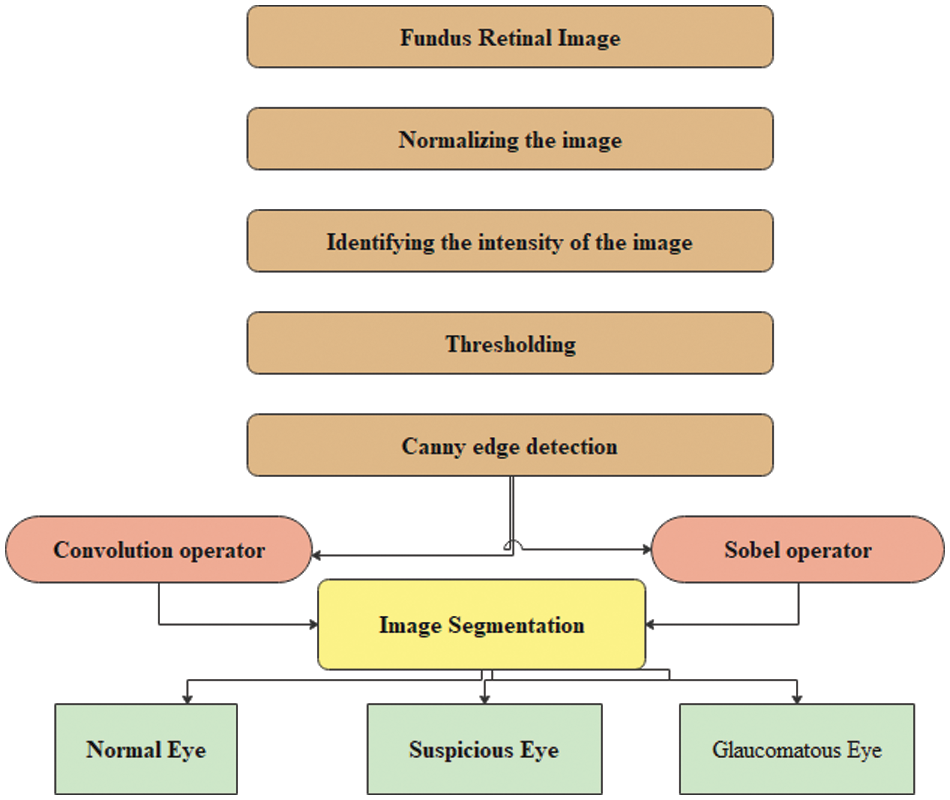
Figure 1: Proposed CNN algorithm for classifying glaucomatous eyes

The selection of the new and modified degree of membership for each fuzzy series of the three partitions based on (x) that was estimated using Eqs. (20)–(21) results in [25].

μI1(x)={1−∏p1=02 μIp1(x)1+∑p1=02 μIp1(x),Λ(x)>012log(1−∑p1=02 μIp1(x)1+∏p1=02 μIp1(x)),Λ(x)≤1(24)

Eq. (24) provided a basis for the membership degrees μIp1(x) that fit the image I1.

3.3 Fuzzy Difference Equation Manipulation and Defuzzification

Fuzzy manipulation functions were obtained by using Eq. (20) to improve the contrast of the retinal image.

μ´I1(x)={2∗μI1(x)2forμI1(x)>0.5;1−2∗(1−μI1(x))2for μI1(x)≤0.5;

μ´I2(x)={2∗μI2(x)2forμI2(x)>0.5;1−2∗(1−μI2(x))2for μI2(x)≤0.5;

μ´I2(x)={2∗μI3(x)2forμI3(x)>0.5;1−2∗(1−μI3(x))2for μI3(x)≤0.5;(25)

The enhanced retinal images represented for each of the three images by IE1, IE2, and IE3 was achieved by defuzzification of the degree of intensification of membership μ´I1(x)μ´I2(x) and μ´I3(x) from Eq. (25) as follows:

 IE1=μI1(x)+∇μ´I1(x)∗(xmax−xmin)

 IE2=μI2(x)+∇μ´I2(x)∗(xmax−xmin)

IE3=μI3(x)+∇μ´I3(x)∗(xmax−xmin)(26)

where ∇μ´I1(x)=μI1(x)−μ´I1(x)

μI1(x)=xij−xminxmax−xmin.

∇μ´I2(x), μI2(x) and ∇μ´I3(x), μI3(x) could also be defined similarly. In these equations,  xmax and xmin are the maximum and minimum concentration levels of the images I1,  I2 and I3.

4  Image Segmentation Using Fuzzy Differential Equations

Fuzzy integrals based on the method of combining a fuzzy image region with different fuzzy characteristics have been used in nonlinear image processing (region, edge detection, histogram, and analyzer) for segmentation. These are used to recursively combine the regions based on the maximum and minimum fuzzy integral [26]. The goal of integrating the regions is to combine the fuzzy targets, and evidence of the fuzzy measurement is reflected in the image regions. The proposed retinal image processing algorithm is shown in Fig. 2 and the implementation of the proposed algorithm was achieved as depicted in Figs. 3–5.

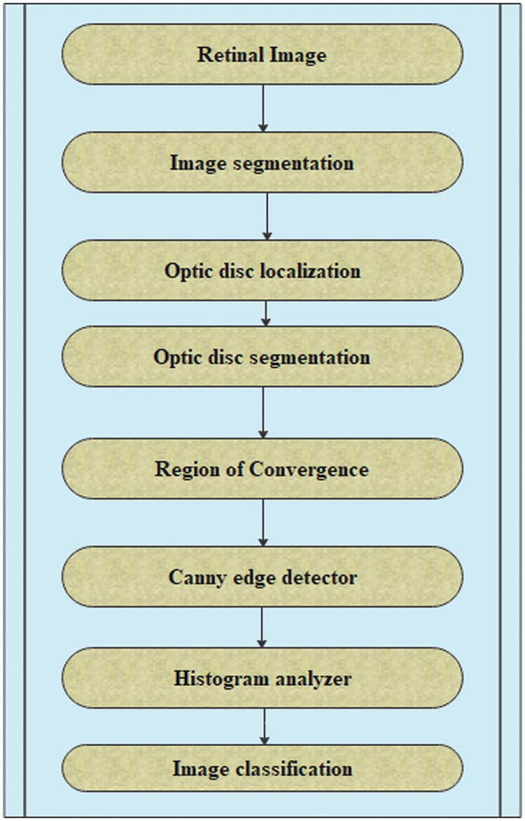
Figure 2: Algorithm for retinal image processing

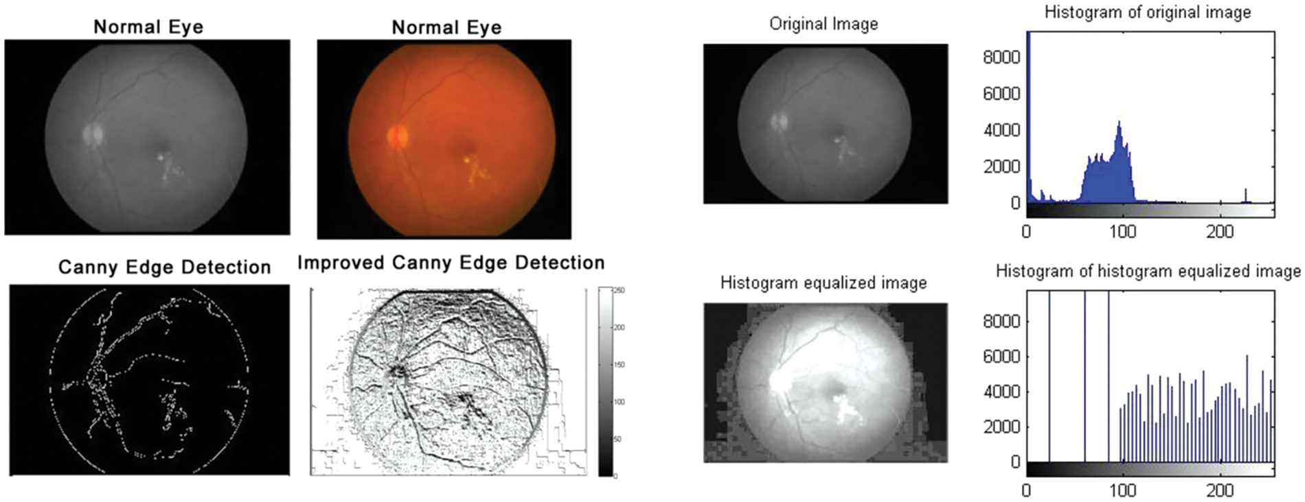
Figure 3: Normal eyes: Edge detection and histogram of histogram equalized image

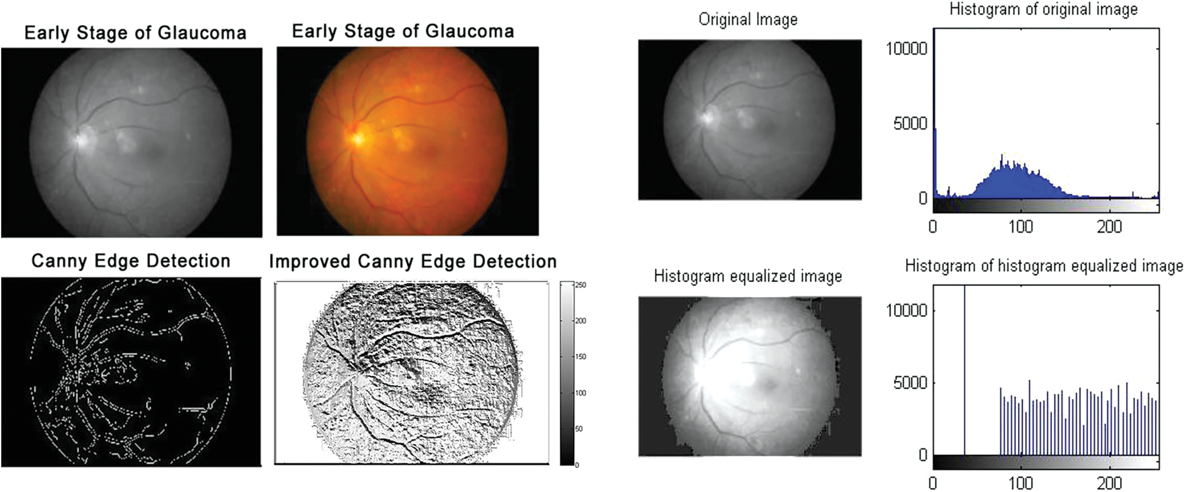
Figure 4: Early-stage glaucomatous eyes: Edge detection and histogram of histogram equalized image

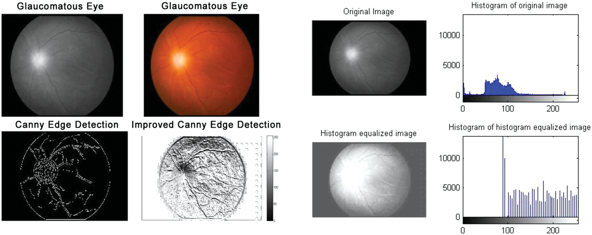
Figure 5: Glaucomatous eyes: Edge detection and histogram of histogram equalized image

Let X1 = {x1,x2, . . . ,xn } be a compilation of data sources, a fuzzy measure is a function of the real value μ defined as μIi:2x→[0, 1] in the set of the family μIi, μI2, and μI3 which is used to segment the images. The fuzzy density measure is μδ and it can be measured as

δ+1=∏i=1n(1+δμIi)(27)

The calculation of fuzzy integral for image segmentation in Eq. (22), δ represents the characteristics of the image as there are different intensities for the various regions [27]. The proposed algorithm is used to measure the fuzziness and the fuzzy integral to connect different regions of partitioning with similar and dissimilar concentration levels.

4.1 Fuzzy Differential Equations’ Calculations

The predictable three fuzzy partitions sets were defined as Ip1(x), Ip2(x), and Ip3(x). The resultant membership degrees of this fuzzy partitions set include µIp1(x), µIp2(x), and µIp3(x). These partition sets contained different concentration levels with their own membership degree. Edge detection, contour detection, and histogram analyzer were used in these three groups of partitions and defined a set of objectives that enclosed the merged information. Three values of fuzzy density were then estimated using the three segments of µIp1(x) and the variables ap1, where p1 = {0, 1, 2} as follows:

a0=μ0(x) a1=μ1(x) a2=μ2(x)(28)

The three fuzzy density values were estimated to be {g0,g1,g2} based on the following conditions:

g0=max(a0, a1),

g1=max(a1, a2)

g2=max(a2, a0).

Now, the characteristic of image δ could be obtained using the three characterized fuzzy densities {g0,g1,g2} for the measurement of the Sugeno-type inference. Replacing the values of {a0,a1,a2} in Eq. (20), and solving the quadratic equation, we get

a=a0a1a2

b=a0a1+a1a2+a0a2

c=(a0+a1+a2−1)(29)

Therefore, any of the skills in the set of measures μIp1(x), p1= {0, 1, 2} in Eq. (16) must be used to estimate the value of δ. Since {g0,g1,g2} and δ are now known based on the fuzzy measurement, the tests on the fuzzy densities could be calculated using the following equations:

g01={g0 ∪g1}=g0+g1+δg0g1

g12={g1∪g2}=g1+g2+δg1g2

g02={g0∪g2}=g0+g2+δg0g2(30)

After measuring the fuzzy density in the set of {a0, a1, a2}, the measurable function h(x) is calculated as follows:

h(x0)=min(a0,g0)

h(x1)=min(a1,g1)

h(x2)=min(a2,g2)(31)

The above three equations must satisfy h(x0)≥h(x1)≥h(x2) condition. Finally, the set of fuzzy density and the measurable function h(x) satisfying h(x0)≥h(x1)≥h(x2) could be used in the fuzzy integral set and then the performance could be determined using Eq. (21), as follows:

μ´IF1(x)=maxi=1,2,…,n[min{h(xi), gi,i+1(x)](32)

where μ´IF1(x) is a fused fuzzy matrix containing an integrated degree of membership of three series of fuzzy partitions {I0, I1, I2}. Furthermore, IF1, IF2, and IF3 are the input eye images.

The degree of belonging could be classified as an object in two classes C0R0, and C1R1 where R0,1 are the regions of the image. It could also be assumed that if any μ´IF1(x)C0 is a member of R0 then μ´IF1(x) is assigned and μ´IF2,3(x)=  0 otherwise, μ´IF1(x) = 1 for the class of C1R1.

The degree of belonging could be classified as an object in two classes C0R0, and C1R1 where R0,1 are the regions of the image. It could also be assumed that if any μ´IF1(x)C0 is a member of R0 then μ´IF1(x) is assigned and μ´IF2,3(x)=  0 otherwise, μ´IF1(x) = 1 for the class of C1R1.

Therefore, an object could belong to the class C0R0 or C1R1 depending on the commencement. The edge ζ from the combined fuzzy matrix μ´IF1(x) could now be calculated using the following two rules:

R0:μ´IF1(x)<ζ|μ´IF1(x)=0 ∈C0(33)

R1:μ´IF1(x)<ζ|μ´IF1(x)=0 ∈C1(34)

where ζ is defined as ζ =13(M×N)∑μ´IF1(x).

4.2 Defuzzification

The segmented retinal image ID1 after the defuzzification process that was described in the previous section is provided as follows:

ID1=μ´IF1(x)∗(xmax−xmin)(35)

where ID1 is the segmented image of the retina in color.

5  Results and Discussion

According to the proposed algorithm, which is illustrated in Figs. 1 and 2, the following were applied to the sample images. Canny edge detection, histogram equalized images, histogram of original images, and histogram of histogram equalized images were classified for normal eyes, early-stage glaucomatous eyes, and glaucomatous eyes as shown in Figs. 3–5.

To assess objective improvement, we used the fuzzy spatial frequency metric along with a canny edge detector to analyze the execution of the proposed strategy towards the parameters of the area of the disc of the age group of 30–40-year-olds and 41–50-year-olds. The corresponding disc diameters (both horizontal and vertical discs), temporal inferior, temporal superior, and nasal were taken as parameters. Sample data for 20 individuals were analyzed and the results are presented in Table 2 and illustrated in Fig. 6.

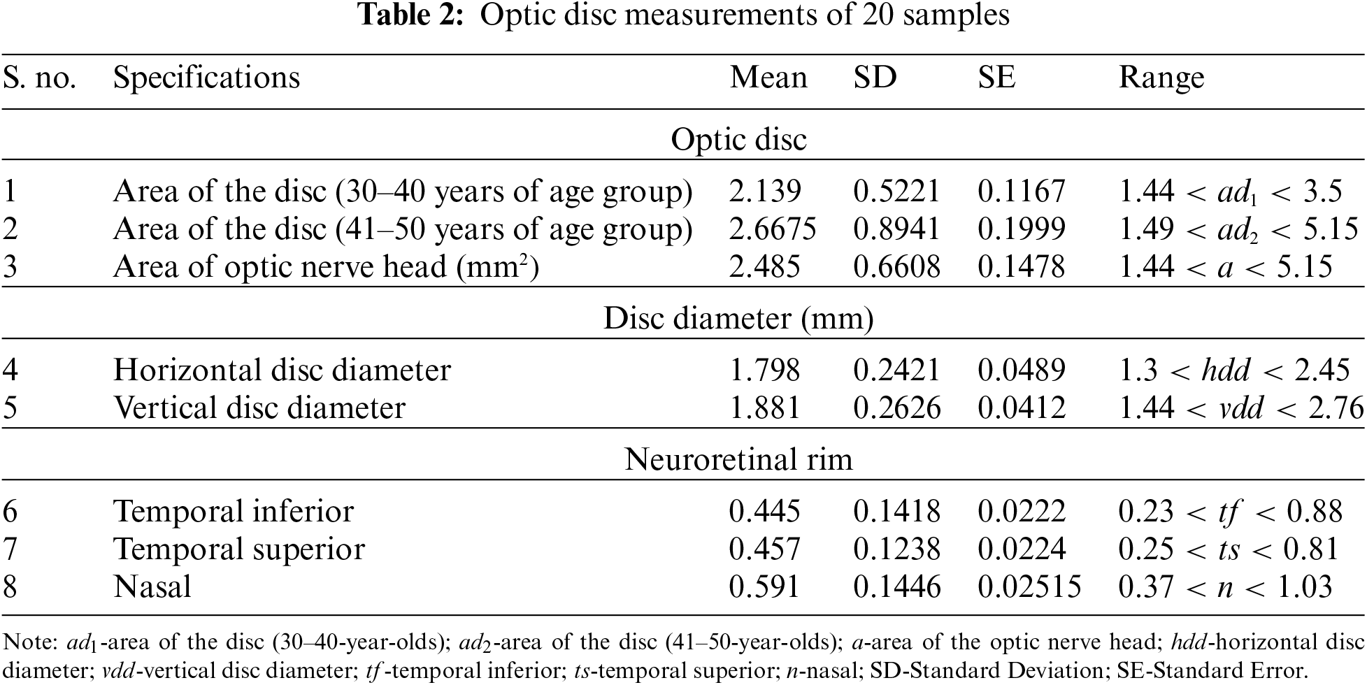
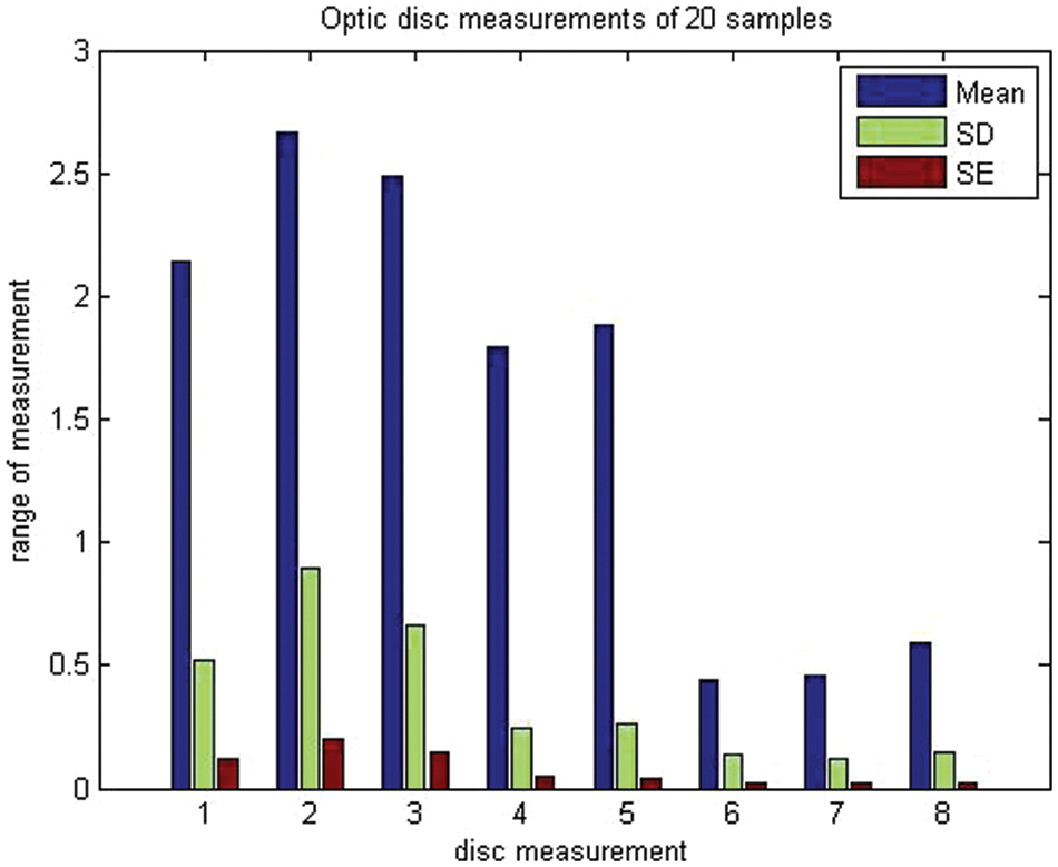
Figure 6: Mean, standard deviation, and standard error of optic disc measurements of 20 samples describing their mean, standard deviation and standard error

In general, according to the algorithm of retinal image processing which was shown in Fig. 2, the spatial recurrence was assessed based on the standard level of visual clarity. When the spatial recurrence was determined to be a high value, which indicated better vision,

F=(RF2+CF2)(36)

where R represents the row frequency (a horizontal measurement of CDR) and C represents the frequency column (a vertical measurement of CDR), M×N is defined by the matrix IF1 which is used to calculate the CDR value and the corresponding standard error as follows:

 RF1=1M(N−1)∑i=0M−1∑i=0N−1(IF1(i,j+1)−IF1(i,j))2(37)

CF1=1M(N−1)∑i=0M−1∑i=0N−1(IF1(i+1,j)−IF1(i,j))2 

Similarly, IF2 and IF3 could also be better estimated using the following equations:

RF2=1M(N−1)∑i=0M−1∑i=0N−1(IF2(i,j+1)−IF2(i,j))2

CF2=1M(N−1)∑i=0M−1∑i=0N−1(IF2(i+1,j)−IF2(i,j))2(38)

RF3=1M(N−1)∑i=0M−1∑i=0N−1(IF3(i,j+1)−IF3(i,j))2

 CF3=1M(N−1)∑i=0M−1∑i=0N−1(IF3(i+1,j)−IF3(i,j))2 (39)

Thus, Eqs. (37)–(39) along with Eqs. (24)–(26) could be used to categorize the eye condition of the patient. The validation of this categorization was then validated through hypothetical medical information, such as optic disc area, disc diameter, and neuroretinal rim values. Row and column frequencies were also used to obtain and classify the range of the region of convergence of the retinal images.

6  Conclusions

A novel approach for the detection of a glaucomatous eye using intuitive fuzzy sets with membership and non-membership functions was discussed in this study. This was accomplished by utilizing intuitive fuzzy (optimal classifier) sets in the region of convergence of the partitioned retinal images. Fuzzy degrees and fuzzy weighted values were then used as the concentration level in the retinal images. Once the concentration levels of the retinal images were found, the image was then classified as normal eyes, suspected glaucomatous eyes, or glaucomatous eyes. The measurement of the concentration level and checking for similarities in different regions of the images generated a threshold image from the combined fuzzy matrix along with the spatial frequency fuzzy metric which led to the precise classification of the eye condition. Canny edge detection, a histogram equalized image, a histogram of original images and a histogram of histogram equalized images were classified for normal eyes, early-stage glaucomatous eyes, and glaucomatous eyes. These techniques were assorted through the proposed deep learning algorithm using the Convolutional Neural Network. Based on this analysis, the intuitionistic fuzzy sets were carried out on a similar pattern identifier envisaged by models of human perception.

Acknowledgement: The authors express their appreciation to King Saud University for funding the publication of this research through the Researchers Supporting Program (RSPD2023R809), King Saud University, Riyadh, Saudi Arabia.

Funding Statement: This research was funded by the Researchers Supporting Program at King Saud University (RSPD2023R809), Riyadh, Saudi Arabia.

Author Contributions: Dorathy Prema Kavitha, L. Francis Raj, Sandeep Kautish and Abdulaziz S. Almazyad conceived of the presented idea. D. Dorathy Prema Kavitha and L. Francis Raj developed the theory and performed the computations. Sandeep Kautish, Abdulaziz S. Almazyad, Karam M. Sallam, and Ali Wagdy Mohamed verified the analytical methods. Sandeep Kautish, Abdulaziz S. Almazyad encouraged D. Dorathy Prema Kavitha and L. Francis Raj to investigate the proposed method and supervised the findings of this work. All authors discussed the results, contributed to, and approved the final manuscript.

Availability of Data and Materials: Not applicable.

Conflicts of Interest: The authors declare that they have no conflicts of interest to report regarding the present study.

References

1. Tjandrasa, H., Wijayanti, A., Suciati, N. (2012). Optic nerve head segmentation using hough transform and active contours. Telkomnika, 10(3), 531–536. https://doi.org/10.12928/telkomnika.v10i3.833 [Google Scholar] [CrossRef]

2. Zhang, M., Chen, Y., Lin, J. (2021). A Privacy-preserving optimization of neighborhood-based recommendation for medical-aided diagnosis and treatment. IEEE Internet of Things Journal, 8(13), 10830–10842. https://doi.org/10.1109/JIOT.2021.3051060 [Google Scholar] [CrossRef]

3. Haubecker, H., Tizhoosh, H. R. (1999). Fuzzy image processing. In: Computer vision and applications. New York: Academic Press. [Google Scholar]

4. Dehghani, A., Moghaddam, H. A., Moin, M. S. (2012). Optic disc localization in retinal images using histogram matching. EURASIP Journal on Image and Video Processing, 2012(1), 19. https://doi.org/10.1186/1687-5281-2012-19 [Google Scholar] [CrossRef]

5. Naik, S. K., Murthy, C. A. (2003). Hue-preserving color image enhancement without gamut problem. IEEE Transactions on Image Processing, 12(12), 1591–1598. https://doi.org/10.1109/TIP.2003.819231 [Google Scholar] [PubMed] [CrossRef]

6. Fard, O. S., Bidgoli, T. A., Rivaz, A. (2017). On existence and uniqueness of solutions to the fuzzy dynamic equations on time scales. Mathematical and Computational Applications, 22(1), 16. [Google Scholar]

7. Rahman, G., Din, Q., Faizullah, F., Khan, F. M. (2018). Qualitative behavior of a second-order fuzzy difference equation. Journal of Intelligent and Fuzzy Systems, 34(1), 745–753. [Google Scholar]

8. Sharma, S., Wasson, E. V. (2015). Retinal blood vessel segmentation using fuzzy logic. Journal of Network Communications and Emerging Technologies (JNCET), 4(3), 1–5. [Google Scholar]

9. Soltani, A., Battikh, T., Jabri, I., Lakhoua, N. (2018). A new expert system based on fuzzy logic and image processing algorithms for early glaucoma diagnosis. Biomedical Signal Processing and Control, 40, 366–377, https://doi.org/10.1016/j.bspc.2017.10.009 [Google Scholar] [CrossRef]

10. Welfer, D., Scharcanski, J., Kitamura, C. M., Dal Pizzol, M. M., Ludwig, L. W. B. et al. (2010). Segmentation of the optic disk in color eye fundus images using an adaptive morphological approach. Computers in Biology and Medicine, 40(2), 124–137. https://doi.org/10.1016/j.compbiomed.2009.11.009 [Google Scholar] [PubMed] [CrossRef]

11. Paulus, J., Meier, J., Bock, R., Hornegger, J., Michelson, G. (2010). Automated quality assessment of retinal fundus photos. International Journal of Computer Assisted Radiology and Surgery, 5, 557–564. https://doi.org/10.1007/s11548-010-0479-7 [Google Scholar] [PubMed] [CrossRef]

12. Atanassov, K. T. (1986). Intuitionistic fuzzy sets. Fuzzy Sets and Systems, 20(1), 87–96. https://doi.org/10.1016/S0165-0114(86)80034-3 [Google Scholar] [CrossRef]

13. Li, Q., You, J., Zhang, D. (2012). Vessel segmentation and width estimation in retinal images using multi scale production of matched filter responses. Expert Systems with Applications, 39, 7600–7610. https://doi.org/10.1016/j.eswa.2011.12.046 [Google Scholar] [CrossRef]

14. Li, Y., Du, L., Wei, D. (2022). Multiscale CNN based on component analysis for SARATR. IEEE Transactions on Geoscience and Remote Sensing, 60, 1–12. https://doi.org/10.1109/TGRS.2021.3100137 [Google Scholar] [CrossRef]

15. Vostatek, P., Claridge, E., Uusitalo, H., Hauta-Kasari, M., Falt, P. et al. (2017). Performance comparison of publicly available retinal blood vessel segmentation methods. Computerized Medical Imaging and Graphics, 55, 2–12. https://doi.org/10.1016/j.compmedimag.2016.07.005 [Google Scholar] [PubMed] [CrossRef]

16. Gour, N., Khanna, P. (2019). Automated glaucoma detection using GIST and pyramid histogram of oriented gradients (PHOG) descriptors. Pattern Recognition Letters, 137, 3–11. https://doi.org/10.1016/j.patrec.2019.04.004 [Google Scholar] [CrossRef]

17. Fraz, M. M., Remagnino, P., Hoppe, A., Uyyanonvara, B., Rudnicka, A. R. et al. (2012). Blood vessel segmentation methodologies in retinal images–A survey. Computer Methods and Programs in Biomedicine, 108(1), 407–433. https://doi.org/10.1016/j.cmpb.2012.03.009 [Google Scholar] [CrossRef]

18. Alamin, A., Mondal, S. P., Alam, S., Goswami, A. (2020). Solution and stability analysis of non-homogeneous difference equation followed by real life application in fuzzy environment. Sādhanā, 45, 185. https://doi.org/10.1007/s12046-020-01422-1 [Google Scholar] [CrossRef]

19. Mjahed, O., Hadaj, S. E., Mahdi, E., Mjahed, S. (2023). Improved supervised and unsupervised metaheuristic-based approaches to detect intrusion in various datasets. Computer Modeling in Engineering & Sciences, 137(1), 265–298. https://doi.org/10.32604/cmes.2023.02758 [Google Scholar] [CrossRef]

20. Sun, T., Su, G., Han, C. H., Zeng, F. P., Qin, B. (2022). Eventual periodicity of a system of max-type fuzzy difference equations of higher order. Fuzzy Sets and Systems, 443, 286–303. [Google Scholar]

21. Hoover, A., Goldbaum, M. (2003). Locating the optic nerve in a retinal image using the fuzzy convergence of the blood vessels. IEEE Transactions on Medical Imaging, 22(8), 951–958. https://doi.org/10.1109/TMI.2003.815900 [Google Scholar] [PubMed] [CrossRef]

22. Huang, M. L., Chen, H. Y., Huang, J. J. (2007). Glaucoma detection using adaptive neuro-fuzzy inference system. Expert Systems with Applications, 32, 458–468. https://doi.org/10.1016/j.eswa.2005.12.010 [Google Scholar] [CrossRef]

23. Thakur, N., Juneja, M. (2018). Survey on segmentation and classification approaches of optic cup and optic disc for diagnosis of Glaucoma. Biomedical Signal Processing and Control, 42, 162–189. https://doi.org/10.1016/j.bspc.2018.01.014 [Google Scholar] [CrossRef]

24. Rajchakit, G., Agarwal, P., Ramalingam, S. (2021). Stability analysis of neural networks. Singapore: Springer. https://doi.org/10.1007/978-981-16-6534-9Se [Google Scholar] [CrossRef]

25. Hanmandlu, M., Jha, D. (2006). An optimal fuzzy system for color image enhancement. IEEE Transactions on Image Processing, 15(10), 2956–2966. https://doi.org/10.1109/TIP.2006.877499 [Google Scholar] [PubMed] [CrossRef]

26. Hussain, S. A., Holambe, A. N. (2015). Automated detection and classification of Glaucoma from eye fundus images: A survey. International Journal of Computer Science and Information Technologies, 6(2), 1217–1224. [Google Scholar]

27. Rajchakit, G., Sriraman, R. (2021). Robust passivity and stability analysis of uncertain complex-valued impulsive neural networks with time-varying delays. Neural Processing Letters, 53, 581–606. [Google Scholar]