
 Submit a Paper
 Propose a Special lssue
 Open Access
ARTICLE

An Efficient Local Radial Basis Function Method for Image Segmentation Based on the Chan–Vese Model
School of Mathematics and Statistics, Guangdong University of Technology, Guangzhou, 510520, China
* Corresponding Author: Wei Zhao. Email:
(This article belongs to the Special Issue: New Trends on Meshless Method and Numerical Analysis)
Computer Modeling in Engineering & Sciences 2024, 139(1), 1119-1134. https://doi.org/10.32604/cmes.2023.030915
Received 02 May 2023; Accepted 28 July 2023; Issue published 30 December 2023
 View Full Text
 Download PDF
Abstract
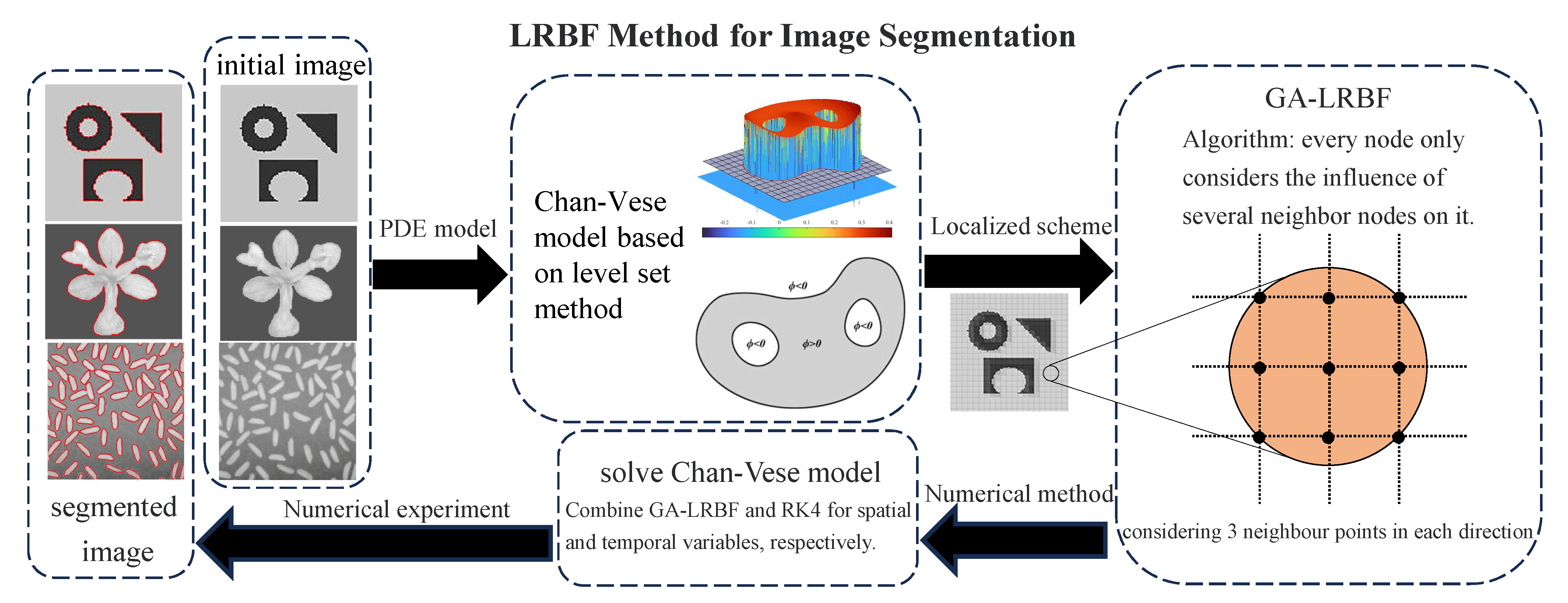
In this paper, we consider the Chan–Vese (C-V) model for image segmentation and obtain its numerical solution accurately and efficiently. For this purpose, we present a local radial basis function method based on a Gaussian kernel (GA-LRBF) for spatial discretization. Compared to the standard radial basis function method, this approach consumes less CPU time and maintains good stability because it uses only a small subset of points in the whole computational domain. Additionally, since the Gaussian function has the property of dimensional separation, the GA-LRBF method is suitable for dealing with isotropic images. Finally, a numerical scheme that couples GA-LRBF with the fourth-order Runge–Kutta method is applied to the C-V model, and a comparison of some numerical results demonstrates that this scheme achieves much more reliable image segmentation.Graphic Abstract
Keywords
Image segmentation is a challenging and complicated task in the field of image processing and has a wide range of applications in computer vision, such as medical image analysis, autonomous driving, remote sensing, security and protection monitoring [1–3]. The major task of image segmentation is to divide a prescribed image into several nonoverlapping and disjoint regions according to characteristics such as color, gray level (intensity) and geometric shape. With the increasing demand for segmentation techniques, many methods have been proposed, including threshold-based methods, region-based methods, edge-based methods, PDE-based methods and emerging methods based on deep neural networks. Among these representative classes of methods, the latter two correspond to mainstream algorithms. Nevertheless, although deep learning methods such as fully convolutional networks perform well in terms of accuracy [4], they are not fully interpretable and require considerable time for neural network training. An image itself can be regarded as a discrete two-dimensional matrix, which can be modeled using continuous mathematical models based on partial differential equations (PDEs). Over the decades, PDE-based models have shown excellent applicability and efficiency due to their high mathematical significance. Among PDE-based models, active contour models are some of the most popular, including the parametric active contour model and the level set method. A parametric active contour model (Snakes) was first proposed by Kass et al. [5]; however, in this model, the curves cannot enter deep areas of the image, and the initial curves must already be close to the edges of the image contours. To handle this limitation, the level set method was presented for flexibly handling topological changes in images [6–9]. In this method, a contour curve is embedded into a higher-dimensional function, representing that the level sets of different topological structures in the evolutionary process all correspond to the same level. Therefore, such a level set function can automatically control topological changes. The Chan–Vese (C-V) model is a typical level set model using a variational principle [10], as an improved variant of the Mumford–Shah (M-S) model [11], in which the complex functional is simplified by assuming that the gray levels within homogeneous regions of an image are constant. Many works have proven that the C-V model can effectively improve the topological adaptation ability in curve evolution; therefore, it is a powerful tool for image segmentation and has attracted increasing attention from researchers [12–14].
Once the desired model has been derived, numerical simulation plays an important role in understanding the dynamic evolutionary process of active contours. At present, the finite differential method (FDM) has been widely applied to numerically solve the PDEs originating from the level set method in most cases; this method achieves reasonably satisfactory accuracy [11] but is computationally expensive. In addition, various traditional techniques and algorithms have been used to optimize the accuracy and results of image segmentation. Nonetheless, limited by the efficiency and data processing ability of these algorithms, many challenges still arise in practical applications. In recent years, the radial basis function (RBF) method has attracted much attention because of its simple format and high accuracy [15–19], and it has gradually developed into a significant numerical method in the scientific computing domain [20–23]. However, for large-scale problems such as image processing, the RBF method incurs excessive computational costs due to the generation of a dense matrix [23–26], and the large condition number of this matrix can also causes calculation instability [27,28]. To conquer this shortcoming, local RBF (LRBF) methods based on positive and conditionally positive global kernels have been developed, such as [29], which consider only the contributions from several neighboring points in the near field while ignoring the influence of distant points. The corresponding sparse interpolation matrix apparently reduces the condition number of the matrix, saves storage space and enhances computational efficiency. Other newly developed local methods, such as [30–32], can also be applied to achieve these benefits.
In this paper, based on a Gaussian (GA) kernel, a new LRBF scheme is developed for solving the C-V model accurately and efficiently. Specifically, since a high-dimensional exponential function can be separated along each dimension, the GA-RBF interpolation can be expressed in the form of a tensor product of multiple one-dimensional interpolations. This approach eliminates the isotropic property of radial basis functions; thus, it is suitable for treating inhomogeneous image problems, and afterward, a local scheme is obtained accordingly.
The remainder of this paper is organized as follows: Section 2 provides a brief review of the C-V segmentation model. Section 3 gives more details of the proposed LRBF method based on a Gaussian kernel and presents a fully discrete system obtained by combining the proposed method with the fourth-order Runge–Kutta method. Several numerical experiments are presented in Section 4 to verify the performance of the proposed method, including its accuracy, efficiency and stability. Finally, some conclusions and plans for further research are reported in Section 5.
In this section, we give a brief review of the C-V model, which is an active contour model for two-phase segmentation based on the Mumford–Shah model. Let
where
In problems of curve evolution, the level set method and, in particular, the ‘motion by mean curvature’ approach of Osher et al. [6] have been used extensively. The curve C is implicitly represented via a Lipschitz function

Figure 1: The level set function graph (left) and the zero-level curve graph (right)
With the introduction of the Heaviside function H and the Dirac measure
the terms in the energy functional have the following forms:
Thus, the energy
By keeping
For the corresponding “degenerate” cases, there are no constraints on the values of
By the calculus of variations, the Gateaux derivative of the functional E can be written as
Therefore, the function
3.1 The Global Radial Basis Function (GRBF) Method
In this section, we introduce the RBF method for the interpolation of scattered data. For a set of N distinct centers
where

Therefore, the following linear system of algebraic equations must be solved:
where
Because it always generates a dense interpolation matrix
3.2 Local Radial Basis Function Method Based on a GA Kernel (GA-LRBF)
For simplicity, we describe the method in two dimensions.
where
From the interpolation conditions on the data points
where
To improve the stability of RBF interpolation, a localized approach was recently developed. The distinctive feature of this method is that only a few neighboring points are needed. Because it generates a sparse interpolation matrix, it consumes less computing time. Specifically, for points
where

Figure 2: The GA-LRBF scheme with
To implement the GA-LRBF method for solving the C-V model, it is necessary to compute the differential operator
which involves spatial derivative terms expressed as
After the GA-LRBF method is applied to the C-V model, it can be expressed as a time-dependent semidiscrete nonlinear system
where
In this section, we consider the fourth-order Runge–Kutta scheme (RK4) for the C-V model. Letting
where
In this section, we report the numerical results obtained from the implementation of the proposed methods in Section 3. For this purpose, we present the following remarks:
• In this paper, all cases are calculated using a time step of
• In practice, we use the regularized Heaviside function
and the corresponding regularized Dirac function
The parameter
• To verify the influence of the initial contour on the subsequent evolution, we consider two types of initial level set functions. One is a circle contour, which is defined as
• To judge the effectiveness of image segmentation, we consider two classical evaluation indices defined as [33,34]
where “DICE” measures the spatial overlap between two target regions A and B and “VOE” describes the error ratio of segmentation. For successful image segmentation, the values of “DICE” and “VOE” should tend toward
Example 4.1. The first term of the C-V model,
Fig. 3 displays the segmentation results for a

Figure 3: Evolution results for the initial image obtained using the GA-LRBF method combined with RK4 with different

Example 4.2. This experiment is designed to test the performance of the LRBF method. For this purpose, we apply the LRBF, GRBF and FDM schemes to discretize the spatial variables of the C-V model and the RK4 scheme for temporal discretization. Both circular and constant initial contours are considered.
Fig. 4 shows the results of the three numerical methods for a

Figure 4: Evolution results of three numerical methods with (a–c) a circular initial contour and (d–f) a constant initial contour

Example 4.3. This experiment is designed to test the performance of RK4. We apply the GA-LRBF method to discretize the spatial variables of the C-V model, and the commonly used forward Euler scheme is introduced for numerical comparison. Two different initial contours (circular and constant) are used.
We select three initial images as shown in Fig. 5. Table 4 lists numerical results of LRBF combined with RK4 and Forward Euler schemes for the edge segmentation problem. As expected, the convergence rate of the RK4 scheme is also much faster than that of the forward Euler scheme. Additionally, for clarity, Figs. 6 and 7 display the contour evolution on these three images. As we can see that, for the edge segmentation problem (Fig. 5a), the forward Euler method with a constant initial contour is less effective than this method with a circular initial contour. In particular, for images with holes (Figs. 5b and 5c), the forward Euler method cannot effectively separate the image from the background regardless of whether a constant or circular initial contour is used. However, RK4 is minimally affected by the above problems.

Figure 5: Three initial images, with pixel of (a)


Figure 6: Evolution results obtained by RK4 (first row) and the forward Euler scheme (second row) with a circular initial contour

Figure 7: Evolution results obtained by RK4 (first row) and the forward Euler scheme (second row) with a constant initial contour
In this paper, we presented a novel numerical method to solve the C-V model arising in image segmentation, in which the GA-LRBF and RK4 schemes were used for spatial and temporal variables, respectively. The LRBF method achieved improved efficiency and stability compared with the standard GRBF method because it used only a few neighboring points rather than all points in the domain. Furthermore, since the extensional function can be separated along each direction, it is suitable for the treatment of inhomogeneous image problems. Numerical results verify that the GA-LRBF method combined with RK4 can guarantee successful segmentation results with both circular and constant initial contours and even for images with holes. Therefore, this method is a powerful numerical tool for image segmentation. At present, the number of neighboring points is fixed for the GA-LRBF method; the question of how to determine the optimal number of points will be a focus of our work in the near future.
Acknowledgement: Authors would like to thank Dr. Rui Zhan at Guangdong University of Technology for providing many valuable suggestions for this research.
Funding Statement: This work was sponsored by Guangdong Basic and Applied Basic Research Foundation under Grant No. 2021A1515110680 and Guangzhou Basic and Applied Basic Research under Grant No. 202102020340.
Author Contributions: Shupeng Qiu: Conceptualization, Methodology, Software, Investigation, Formal Analysis, Writing Original Draft; Chujin Lin: Visualization, Investigation; Wei Zhao: Conceptualization, Funding Acquisition, Resources, Supervision, Writing Review & Editing.
Availability of Data and Materials: The authors confirm that the data supporting the findings of this study are available within the article.
Conflicts of Interest: The authors declare that they have no conflicts of interest to report regarding the present study.
References
1. Bennai, M. T., Guessoum, Z., Mazouzi, S., Cormier, S., Mezghiche, M. (2023). Multi-agent medical image segmentation: A survey. Computer Methods and Programs in Biomedicine, 232, 107444. [Google Scholar] [PubMed]
2. Foucart, A., Debeir, O., Decaestecker, C. (2023). Shortcomings and areas for improvement in digital pathology image segmentation challenges. Computerized Medical Imaging and Graphics, 103, 102155. [Google Scholar] [PubMed]
3. Mrinal, R. B. P. D., Javed, M. S. M. S. (2021). Autonomous driving architectures: Insights of machine learning and deep learning algorithms. Machine Learning with Applications, 6, 100164. [Google Scholar]
4. Long, J., Shelhamer, E., Darrell, T. (2015). Fully convolutional networks for semantic segmentation. IEEE Transactions on Pattern Analysis and Machine Intelligence, 39(4), 640–651. [Google Scholar]
5. Kass, M., Witkin, A., Terzopoulos, D. (1988). Snakes: Active contour models. International Journal of Computer Vision, 1(4), 321–331. [Google Scholar]
6. Osher, S., Sethian, J. A. (1988). Fronts propagating with curvature-dependent speed: Algorithms based on hamilton-jacobi formulations. Journal of Computational Physics, 79(1), 12–49. [Google Scholar]
7. Jeon, M., Alexander, M., Pedrycz, W., Pizzi, N. (2005). Unsupervised hierarchical image segmentation with level set and additive operator splitting. Pattern Recognition Letters, 26(10), 1461–1469. [Google Scholar]
8. Malladi, R., Sethian, J. A., Vemuri, B. C. (2009). Shape modeling with front propagation. Journal of Architecture & Planning, 74(74), 1935–1943. [Google Scholar]
9. Ngo, T. A., Zhi, L., Carneiro, G. (2017). Combining deep learning and level set for the automated segmentation of the left ventricle of the heart from cardiac cine magnetic resonance. Medical Image Analysis, 35, 159–171. [Google Scholar] [PubMed]
10. Mumford, D., Shah, J. (1989). Optimal approximations by piecewise smooth functions and associated variational problems. Communications on Pure & Applied Mathematics, 42(5), 577–685. [Google Scholar]
11. Chan, T. F., Vese, L. A. (2001). Active contours without edges. IEEE Transactions on Image Processing, 10(2), 266–277. [Google Scholar] [PubMed]
12. Xu, C., Li, C., Gui, C., Fox, M. D. (2005). Level set evolution without re-initialization. 2005 IEEE Computer Society Conference on Computer Vision and Pattern Recognition (CVPR’05), pp. 430–436. San Diego, CA, USA, IEEE Computer Society. [Google Scholar]
13. Wang, X. F., Huang, D. S., Xu, H. (2010). An efficient local chan-vese model for image segmentation. Pattern Recognition, 43(3), 603–618. [Google Scholar]
14. Li, Y., Kim, J. (2012). An unconditionally stable numerical method for bimodal image segmentation. Applied Mathematics & Computation, 219(6), 3083–3090. [Google Scholar]
15. Franke, C., Schaback, R. (1998). Solving partial differential equations by collocation using radial basis functions. Applied Mathematics and Computation, 93(1), 73–82. [Google Scholar]
16. Dehghan, M., Shokri, A. (2007). A numerical method for KdV equation using collocation and radial basis functions. Nonlinear Dynamics, 54(1), 136–146. [Google Scholar]
17. Majdisova, Z., Skala, V. (2018). Radial basis function approximations: Comparison and applications. Applied Mathematical Modelling, 51, 728–743. [Google Scholar]
18. Dereli, Y., Schaback, R. (2013). The meshless kernel-based method of lines for solving the equal width equation. Applied Mathematics & Computation, 219(10), 5224–5232. [Google Scholar]
19. Lenarduzzi, L., Schaback, R. (2017). Kernel-based adaptive approximation of functions with discontinuities. Applied Mathematics & Computation, 307, 113–123. [Google Scholar]
20. Rad, J. A., Hook, J., Larsson, E., von Sydow, L. (2017). Forward deterministic pricing of options using Gaussian radial basis functions. Journal of Computational Science, 24, 209–217. [Google Scholar]
21. Lotfi, Y., Parand, K. (2022). Efficient image denoising technique using the meshless method: Investigation of operator splitting RBF collocation method for two anisotropic diffusion-based PDEs. Computers & Mathematics with Applications, 113, 315–331. [Google Scholar]
22. Zhao, S., Oh, S. K., Kim, J. Y., Fu, Z., Pedrycz, W. (2022). Motion-blurred image restoration framework based on parameter estimation and fuzzy radial basis function neural networks. Pattern Recognition, 132, 108983. [Google Scholar]
23. Xie, X., Mirmehdi, M. (2011). Radial basis function based level set interpolation and evolution for deformable modelling. Image and Vision Computing, 29(2–3), 167–177. [Google Scholar]
24. Kashyap, K. L., Bajpai, M. K., Khanna, P. (2017). Globally supported radial basis function based collocation method for evolution of level set in mass segmentation using mammograms. Computers in Biology and Medicine, 87, 22–37. [Google Scholar] [PubMed]
25. Li, S., Li, X. (2016). Radial basis functions and level set method for image segmentation using partial differential equation. Applied Mathematics and Computation, 286, 29–40. [Google Scholar]
26. Gelas, A., Bernard, O., Friboulet, D., Prost, R. (2007). Compactly supported radial basis functions based collocation method for level-set evolution in image segmentation. IEEE Transactions on Image Processing, 16(7), 1873–1887. [Google Scholar] [PubMed]
27. Chen, C. S., Noorizadegan, A., Young, D. L., Chen, C. S. (2023). On the selection of a better radial basis function and its shape parameter in interpolation problems. Applied Mathematics and Computation, 442, 127713. [Google Scholar]
28. Ghalichi, S. S. S., Amirfakhrian, M., Allahviranloo, T. (2022). An algorithm for choosing a good shape parameter for radial basis functions method with a case study in image processing. Results in Applied Mathematics, 16, 100337. [Google Scholar]
29. Zhao, W., Hon, Y. C., Stoll, M. (2018). Localized radial basis functions-based pseudo-spectral method (LRBF-PSM) for nonlocal diffusion problems. Computers & Mathematics with Applications, 75(5), 1685–1704. [Google Scholar]
30. Zheng, Z., Li, X. (2022). Theoretical analysis of the generalized finite difference method. Computers & Mathematics with Applications, 120, 1–14. [Google Scholar]
31. Wang, F., Khan, M. N., Ahmad, I., Ahmad, H., Abu-Zinadah, H. et al. (2022). Numerical solution of traveling waves in chemical kinetics: Time-fractional fishers equations. Fractals, 30(2), 2240051. [Google Scholar]
32. Abbaszadeh, M., Dehghan, M. (2020). An upwind local radial basis functions-differential quadrature (RBFs-DQ) technique to simulate some models arising in water sciences. Ocean Engineering, 197, 106844. [Google Scholar]
33. Chang, H. H., Zhuang, A. H., Valentino, D. J., Chu, W. C. (2009). Performance measure characterization for evaluating neuroimage segmentation algorithms. Neuroimage, 47(1), 122–135. [Google Scholar] [PubMed]
34. Bo, L., Cheng, H. D., Huang, J., Tian, J., Tang, X. et al. (2010). Probability density difference-based active contour for ultrasound image segmentation. Pattern Recognition, 43(6), 2028–2042. [Google Scholar]
Fig. 8 displays the segmentation results for a

Figure 8: Evolution results for the initial image obtained using the GRBF method combined with RK4 with different

Cite This Article
 Copyright © 2024 The Author(s). Published by Tech Science Press.
This work is licensed under a Creative Commons Attribution 4.0 International License , which permits unrestricted use, distribution, and reproduction in any medium, provided the original work is properly cited.
 Downloads
 Citation Tools