
 Submit a Paper
 Propose a Special lssue
 Open Access
ARTICLE

Optimization Algorithms of PERT/CPM Network Diagrams in Linear Diophantine Fuzzy Environment
1 Department of Mathematics, Bannari Amman Institute of Technology, Sathyamangalam, Tamil Nadu, 638401, India
2 Basic Sciences Department, Preparatory Year Deanship, King Faisal University, Al-Ahsa, 31982, Saudi Arabia
3 Department of Mathematics, University of the Punjab, Lahore, Pakistan
4 College of Vestsjaelland South, Herrestraede 11, Slagelse, 4200, Denmark
* Corresponding Author: Ashraf Al-Quran. Email:
Computer Modeling in Engineering & Sciences 2024, 139(1), 1095-1118. https://doi.org/10.32604/cmes.2023.031193
Received 20 May 2023; Accepted 26 July 2023; Issue published 30 December 2023
 View Full Text
 Download PDF
Abstract
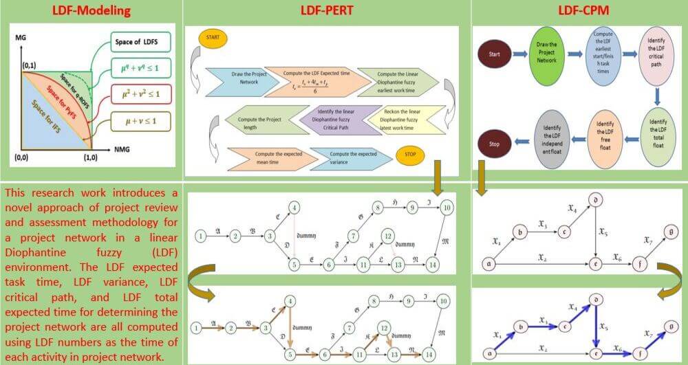
The idea of linear Diophantine fuzzy set (LDFS) theory with its control parameters is a strong model for machine learning and optimization under uncertainty. The activity times in the critical path method (CPM) representation procedures approach are initially static, but in the Project Evaluation and Review Technique (PERT) approach, they are probabilistic. This study proposes a novel way of project review and assessment methodology for a project network in a linear Diophantine fuzzy (LDF) environment. The LDF expected task time, LDF variance, LDF critical path, and LDF total expected time for determining the project network are all computed using LDF numbers as the time of each activity in the project network. The primary premise of the LDF-PERT approach is to address ambiguities in project network activity times more simply than other approaches such as conventional PERT, Fuzzy PERT, and so on. The LDF-PERT is an efficient approach to analyzing symmetries in fuzzy control systems to seek an optimal decision. We also present a new approach for locating LDF-CPM in a project network with uncertain and erroneous activity timings. When the available resources and activity times are imprecise and unpredictable, this strategy can help decision-makers make better judgments in a project. A comparison analysis of the proposed technique with the existing techniques has also been discussed. The suggested techniques are demonstrated with two suitable numerical examples.Graphic Abstract
Keywords
The majority of large projects have a complicated structure and a significant number of contracts between several firms. Controlling the overall project state and making rapid choices might be difficult in these scenarios. As a result, sluggish answers from partners might cause project schedules to be pushed back. It is also crucial since the condition in each project component might impact the total project completion schedule. Through their pre-programmed processes, software applications can coordinate the project’s time and financial management, delay, and reserves. All of this necessitates the fusion of several project management strategies using information symmetry, interaction, risk mitigation, change tracking, and quality maintenance in a dynamic context like time.
The timely completion of a project is contingent on a well-planned timetable. Work Breakdown Structure is a project management method that breaks down a project into activities, or smaller jobs. Each action has its own time limit; it needs preconditioning and yields a result. Activities are also employed in the project scheduling approach, which is determined based on the complexity, size, and urgency of the project. The method must be compact and easy to use. Gantt charts and the critical path approach are two examples of methodologies that satisfy these requirements (CPM). Gantt charts, on the other hand, have limitations when it comes to presenting inter-dependency of activities, in that they do not indicate how one action is dependent on the others. Furthermore, upgrading them takes a long time [1].
The project’s interdependent activities formed an activity network. In a big project, the complexity of the activity network grows fast as the variety of strategies grows. CPM is a network analysis technique that is critical for making sense of a jumble of activity. Nonetheless, CPM is unlikely to be successful in large-scale initiatives. Project activities, on the other hand, are considered to have a range of durations, which are characterized by independent random variables with a specified probability distribution function. Furthermore, they are dynamic, and their intended value may alter under specific conditions. As a result, the Program Evaluation and Review Technique (PERT) was born.
The Critical Path Method (CPM) and the Project Evaluation and Review Technique (PERT) have been two of the most prominent project management techniques for many years. For more than four decades, the latter has been utilized as a project management tool. It entails planning, developing, and executing a series of activities to achieve a certain objective or job.
The CPM was created in the 1950s by Kelly of Remington-Rand and Walker of Dupont to aid in the scheduling of chemical processing plant maintenance and shutdowns. The US Navy quickly created PERT to supervise the development of the Polaris missile [2]. PERT is a strategy being used for projects with activities with stochastic time-frames [3], whereas CPM manages projects with predetermined times. However, practitioners increasingly frequently interchange the two terms or combine them into the acronym PERT/CPM. After 1960, all defense contractors embraced PERT to manage the enormous one-time tasks that the sector entailed. Smaller firms that were given federal contracts linked to defense found it vital to employ PERT. Both utilize a graphical and network model of a project to display the tasks, their interdependencies, and time frame.
Zadeh [4] introduced fuzzy set (FS) theory with uncertainty parameters instead of crisp numbers. Under this fuzzy environment, Elizabeth et al. [5] explored a critical path problem. A critical path problem for project networks has been discussed. To identify the essential degrees of activities and routes, the latest and earliest beginning times, and floats, Chen et al. [6] presented a novel approach that integrates fuzzy set theory with the PERT technique. Different CPM/PERT techniques have been developed in recent years based on fuzzy set theory for project management.
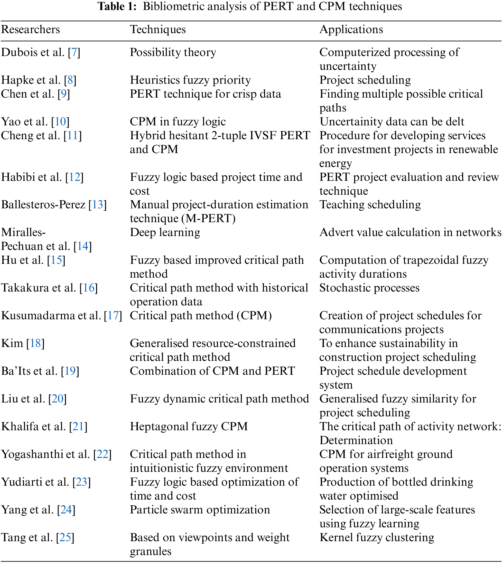
Now we discuss some existing optimization techniques such as PERT and CPM techniques and their applications. Bibliometric analysis of PERT and CPM techniques is expressed in Table 1.
Atanassov [26,27] included another parameter (the non-membership value) to the fuzzy parameter (the membership value) in the year 1999 and it is named as intuitionistic fuzzy set (IFS). Later Jayagowri et al. [28] in 2014 and Kiruthiga et al. [29] in 2019 introduced and studied CPM and PERT concepts, respectively, in the intuitionistic fuzzy environment. New concepts are now possible in Internet-based environments and services thanks to advancements in information and communication technologies. These new concepts can be managed well using PERT and CPM techniques. Yager [30–32] introduced the Pythagorean fuzzy set (PyFS) in 2013. Recently Riaz et al. [33–35] introduced the concept of a linear Diophantine fuzzy set (LDFS) which has unique features and is better compared to the existing sets like FS, IFS and PyFS as it has a wider space and features. Also, it overcomes the limitations in the existing set theories with the reference parameter.
The membership grades (MG) and non-membership grades (NMG) in decision-making are insufficient for analyzing objects in the universe. The incorporation of reference parameters or control parameters gives decision-makers flexibility in choosing these grades. The LDFS, along with its associated reference parameters, provides a robust approach for modeling uncertainties. LDFS removes the limitations of MG and NMG in the existing fuzzy set theories with the idea of control parameters and reference parameters. LDFS provides robust MCDM techniques with new optimization algorithms for information fusion under uncertainty.
Fig. 1 provides a brief overview of the comparison between IFS, PyFS, q-ROFS, and LDFS.
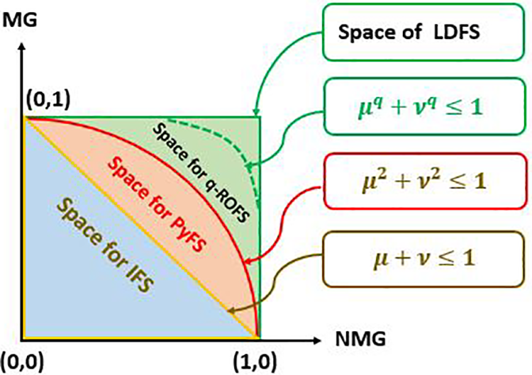
Figure 1: Comparison of IFS, PFS, q-ROFS, and LDFS
LDFS has its unique feature by incorporating the reference parameter and got many real-life applications with the help of different algorithms and operators like Dijkstra algorithm in LDFS environment [36], Einstein aggregation operators for multi-criteria decision-making [37], TOPSIS, VIKOR and Aggregation Operators [38], q-linear Diophantine fuzzy emergency decision support system [39], cosine similarity measures [40]. Also when we consider CPM/PERT got their one results and optimizes the project. But both concepts have not yet been combined. This research gap motivated us to do this paper. There were several significant changes between the early versions of PERT and CPM. They did, however, have a lot of similarities, and the two approaches [41,42] have progressively blended over time. In reality, today’s software packages frequently incorporate all of the key features from both generations. Akram et al. [43] proposed prioritized weighted aggregation operators for complex spherical fuzzy information. Feng et al. [44] developed novel concepts of q-ROFNs for performance evaluation and ranking. Hanif et al. [45] introduced a new MCDM based on LDF graphs. Pamucar [46] proposed Dombi Bonferroni mean normalized weighted geometric operator. Riaz et al. [47] proposed soft-max aggregation operators (AOs) related to LDFSs. Dordevic et al. [48] introduced integrated linear programming fuzzy-rough MCDM model. Ali et al. [49] gave the idea of Einstein Geometric AOs using a complex interval-valued Pythagorean fuzzy set. Al-Quran [50] introduced T-spherical linear Diophantine fuzzy aggregation operators for multiple attribute decision-making. Al-Sharqi et al. [51] proposed the notion of FP-interval complex neutrosophic soft sets and their applications under uncertainty. Many researchers extended fuzzy sets and soft sets to wards MCDM such as T-spherical hesitant fuzzy sets [52], bipolar fuzzy soft sets [53], almost convergence [54], soft union ideals and near-rings [55,56], LDFS sine-trigonometric aggregation operators [57], LBWA and Z-MABAC methods [58].
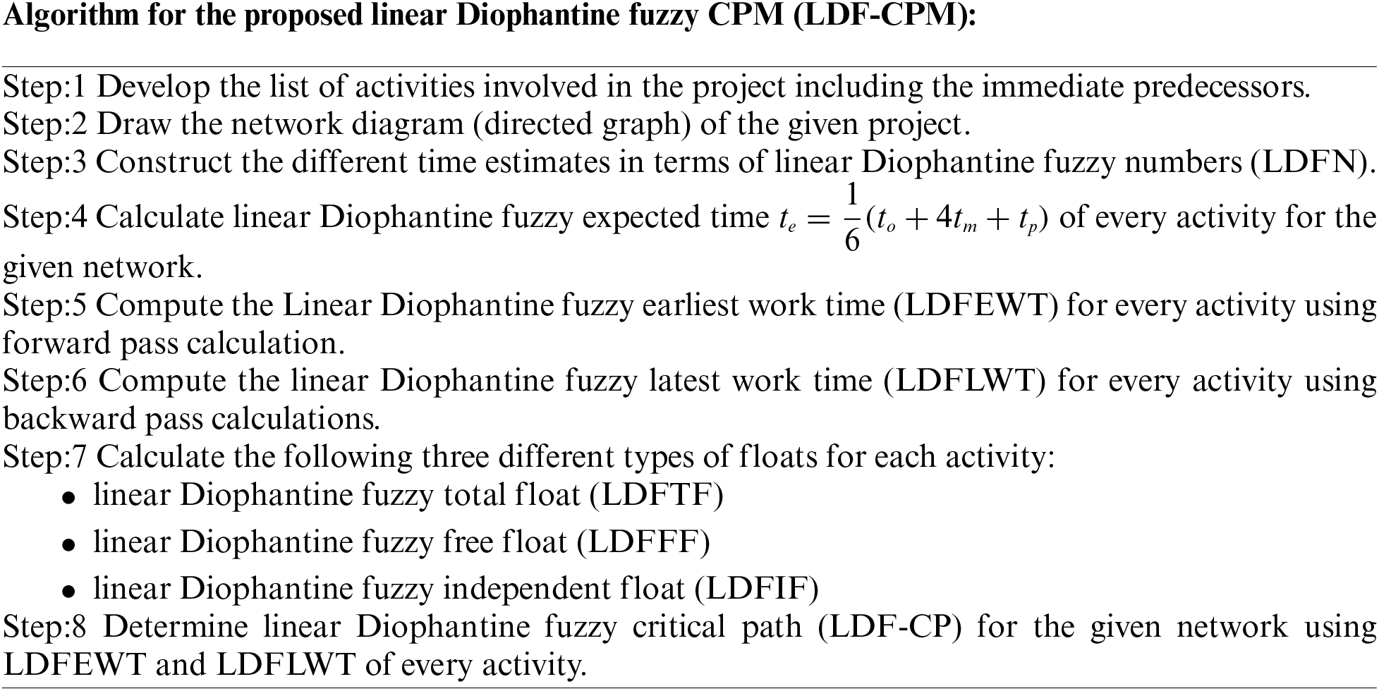
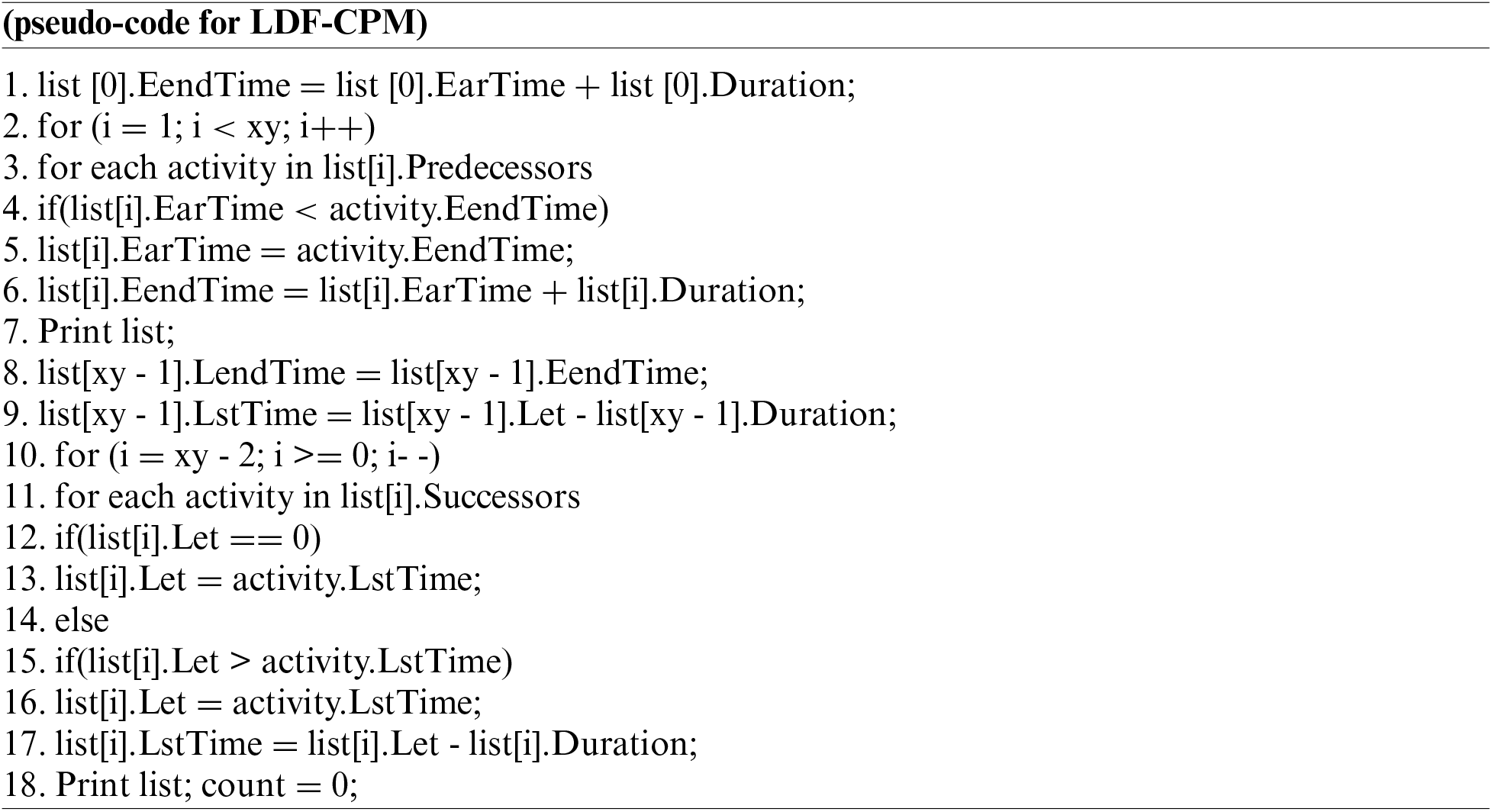
This manuscript aimed to suggest techniques for solving the critical path problem in the LDFG context. The mathematical formulation of CPM/PERT issues is discussed first. Where the time estimates of the traversal of arcs are expressed in terms of Linear Diophantine Fuzzy Numbers (LDFNs). Then, we introduce the Linear Diophantine fuzzy Project Evaluation and Review Technique (LDF-PERT) and Linear Diophantine fuzzy Critical Path Method (LDF-CPM) and two algorithms and pseudo code for the same. A reliable building construction project (BCP) problem and garment production and sales process (GPSP) problem in an LDF setting are used to explain the proposed algorithms.
Project management innovations are required and need to be handled well because the building and textile processes are so complicated. In this context, time management is crucial to the project management process, and methodologies like CPM, PERT, Gantt charts, etc., are employed to establish time-frames. In this study, the LDF-PERT and CPM methodologies were developed and used to analyze problems in the manufacture and sales of clothing as well as infrastructure building projects in order to manage time and identify the critical path.
Delegated project managers must be capable of managing project processes without needless procedures and bureaucratic hurdles because project management in BCP and GPSP problems does not fall under a separate project department made up of multiple experts. Particularly when workers lack sufficient expertise, it is important to offer them a model or guidance that will enable them to complete all project management processes in a symmetrical manner. The suggested methodology is based on the needs of BCP and GPSP problems to provide a tool to support project management that is effective, simple to evaluate, and decreases the risk of errors and negative impacts on the specified objectives, which should support managing the project phases symmetrically. Results showed that our methodology worked well for both BCP and GPSP problems utilizing a symmetric approach to project management.
The main research contributions that were made in order to achieve these objectives are given below:
(i) A brand-new critical path technique is proposed to counteract the effects of both objective and subjective factors.
(ii) The two parameters (satisfaction and dis-satisfaction grades) along with the reference parameters are considered.
(iii) For linear Diophantine fuzzy sets, a novel information measure is introduced via PERT/CPM.
(iv) The three-time estimates of traversal of arcs are calculated and their effects on the ranking of the alternatives are discussed.
(v) To address the comparability problem, a novel score function for linear Diophantine fuzzy numbers is proposed.
(vi) Two launched algorithms are explained elaborately with two real-life quantitative illustrations.
The following is how the rest of the paper is organized: Section 3 covers the basic definitions of fuzzy sets, intuitionistic fuzzy sets, Pythagorean fuzzy sets and some fundamental principles of linear Diophantine fuzzy sets, while Section 4 covers the algorithms, pseudo-code and the flow diagram of the proposed LDF-PERT along with the numerical example in infra building construction project problem that exemplifies the proposed solution methodology. The proposed LDF-CPM algorithm, pseudo-code, flow diagram, and numerical example of garment production & sales process problem, that demonstrates the suggested solution approach are covered in Section 5. Section 6 provides the application and advantages of the proposed techniques. The article is finally concluded in Section 7.
In this section, we recall some essential notions of IFS, PyFs and LDFS.
Definition 3.1. [26] Let
where
Definition 3.2. [30–32] Let
where
Definition 3.3. [33,34] A LDFS
where
Example 3.1. Let
(i)
(ii)
(iii) As for
This shows that LDFS is bigger than IFS and PyFS, and we have more options for assigning values to
Definition 3.4. A LDFS on
(i) absolute LDFS, if it is of the form
(ii) null or empty LDFS, if it is of the form
The null LDFS and absolute LDFS are the smallest and largest LDFSs with respect to score function, respectively. The sets are very helpful in studying the algebraic and topological structures of LDFSs.
Definition 3.5. [33–35] Let
1.
2.
where
Definition 3.6. [33–35] Let
(i)
(ii)
(iii)
(iv)
(v)
(vi)
(vii)
(viii)
(ix)
(x)
(xi)
Example 3.2. Let
(i)
(ii)
(iii)
(iv)
(v)
(vi)
If
(vii)
(viii)
(ix)
(x)
Definition 3.7. Two LDFNs
(i)
(ii)
(iii) If
(a)
(b)
(c)
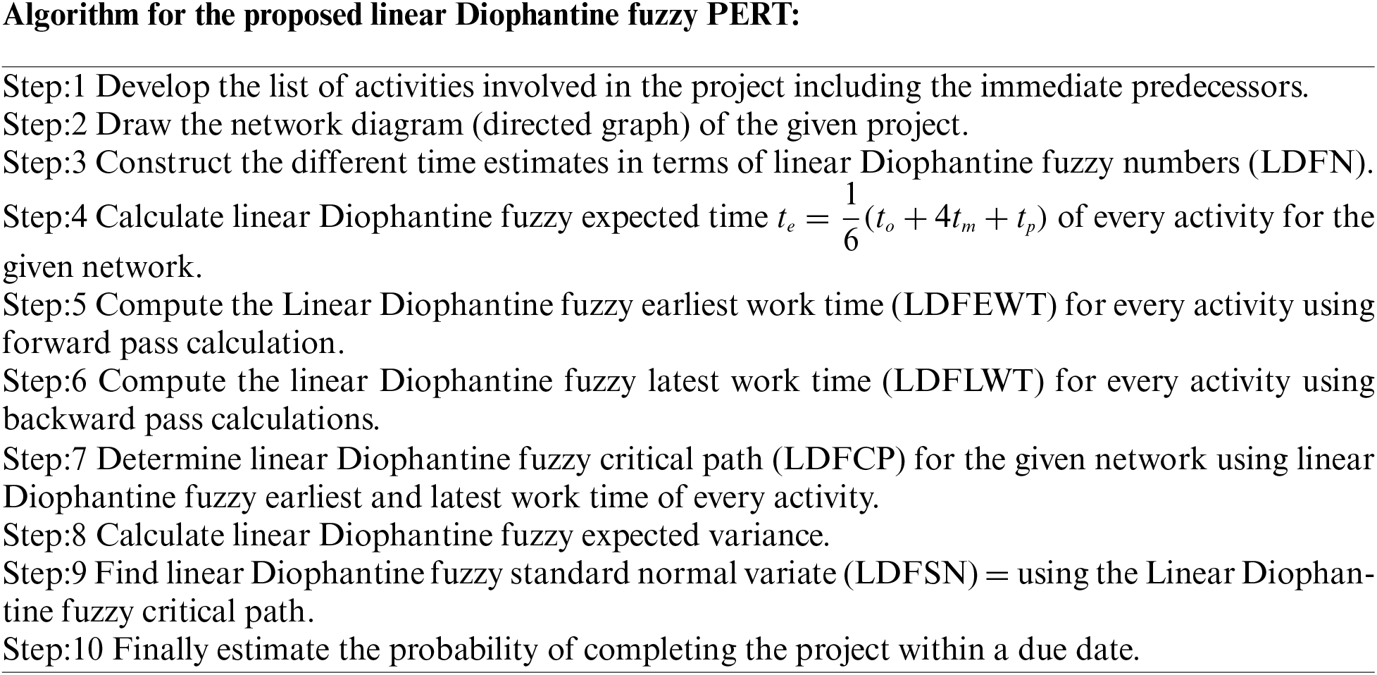
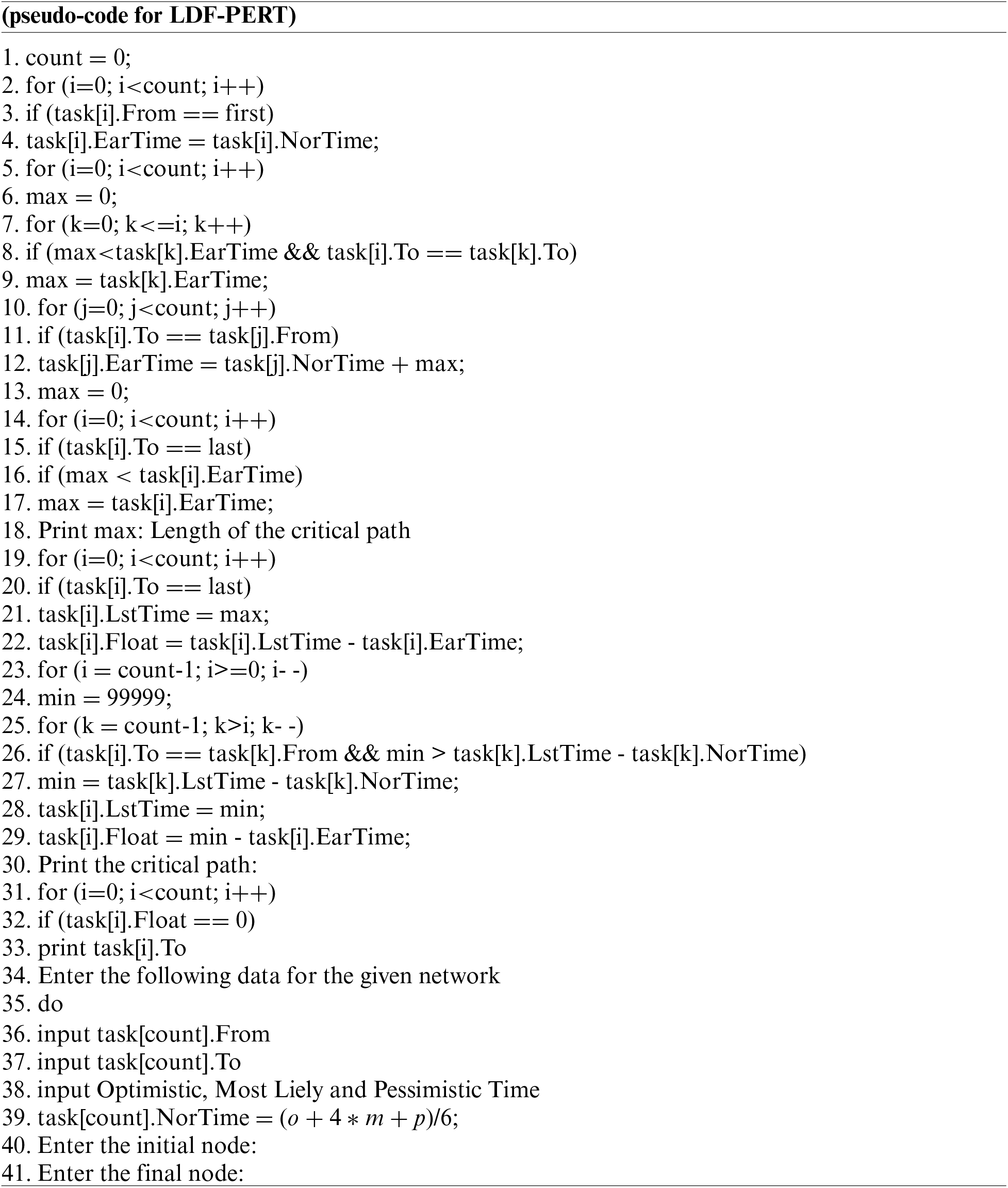
Linear Diophantine fuzzy Project Evaluation and Review Technique (LDF-PERT) algorithm is the generalized fuzzy Project Evaluation an Review Technique based on its predicted LDF-values. In our next Sub-section 4.1, we draft the LDF-PERT algorithm followed by a flow diagram in Fig. 2 and its pseudo-code. Also in Sub-section 4.2, we draft the numerical example for the LDF-PERT.
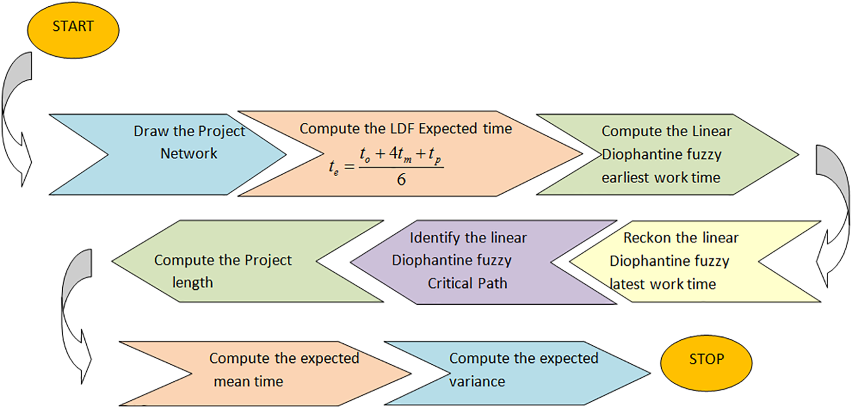
Figure 2: Flow diagram for LDF-PERT
4.1 The PERT Algorithm-Our Extension via LDFG
4.2 Numerical Application for LDF-PERT-Case Study: Infra Building Construction Project Problem
The Infra construction business recently won a $6.5 million contract to build a new factory for a large manufacturer. The factory must be operational within a year, according to the company. As a result, the contract includes the following clauses:
• A $500,000 penalty if Infra does not finish construction by the time-frame of 1 year.
• A bonus of $250,000 will be granted to Infra if the plant is finished in less than 10 months, as an added incentive for quick construction.
Harry Ben, Infra’s finest construction manager, has been assigned to this project to assist keep it on track. He is looking forward to the challenge of finishing the project on time, if not ahead of schedule. However, because he doubts that completing the project in 10 months without incurring exorbitant expenditures will be possible, he has opted to focus his first planning on meeting the deadline of 12 months.
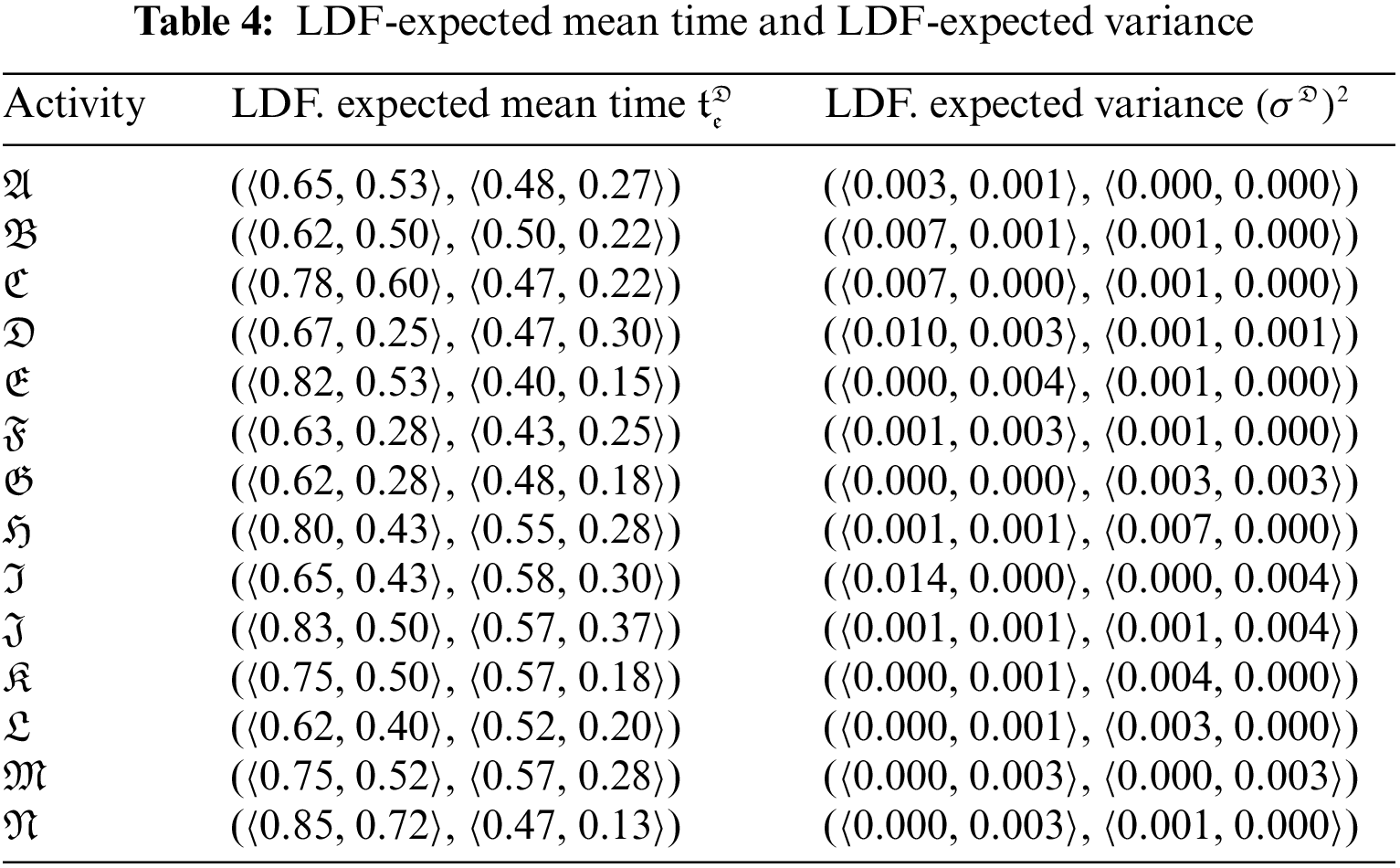
Mr. Ben will have to coordinate a number of workers to complete the various construction tasks at various times. His list of activities is shown in Table 2. The third column contains crucial supplementary information (immediate predecessors) for organizing crew schedule. For every given activity, its immediate predecessors (as indicated in the third column of Table 2) are those actions that must be finished by no later than the commencement time of the given activity. Similarly, the provided action is termed an immediate successor of each of its immediate predecessors. LDFWT for the Activity list of the construction project is given in Table 3. Network diagram of the proposed work flow is expressed in Fig. 3. LDF-Expected mean time and LDF-Expected variance is expressed in Table 4.
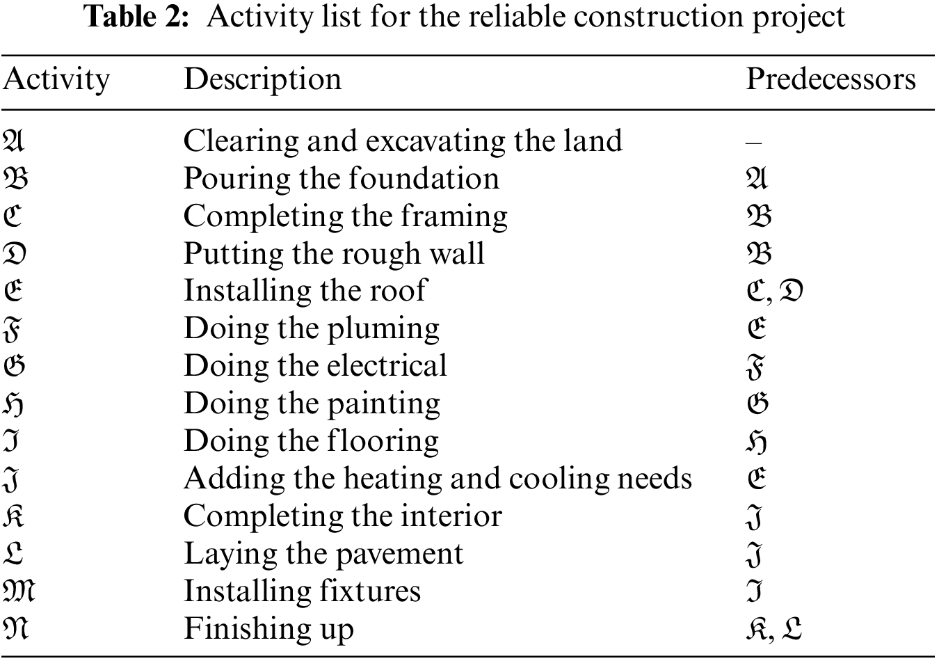
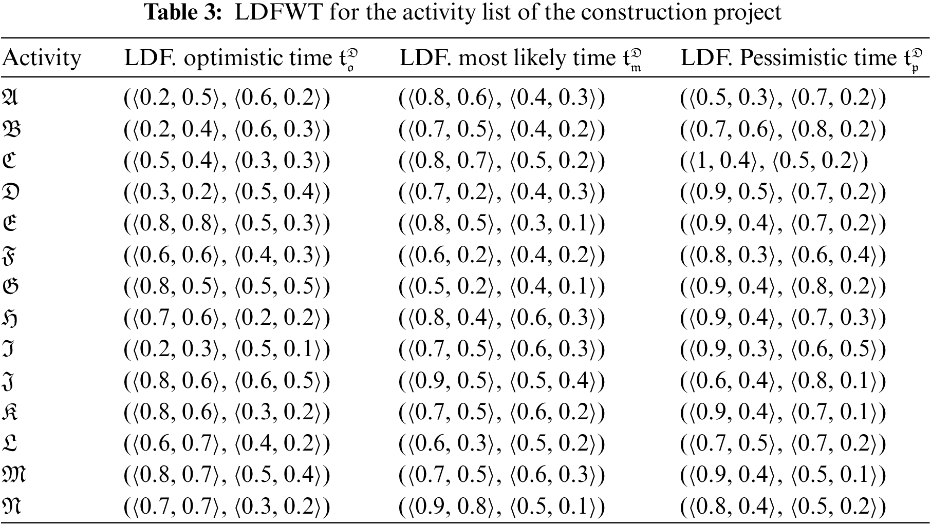
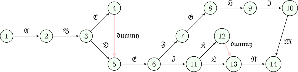
Figure 3: Network diagram of the proposed work flow
4.2.1 Linear Diophantine Fuzzy Earliest Start Task Times
•
•
•
•
•
•
•
•
•
•
•
•
•
•
4.2.2 Linear Diophantine Fuzzy Latest Finishing Task Times
• Let
•
•
•
•
•
•
•
•
•
•
•
•
•
4.2.3 Results and Discussion for the Infra Building Construction Project Problem
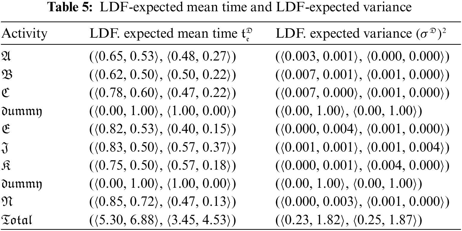
From Sections 4.2.1 and 4.2.2, we conclude that the linear Diophantine fuzzy critical path is
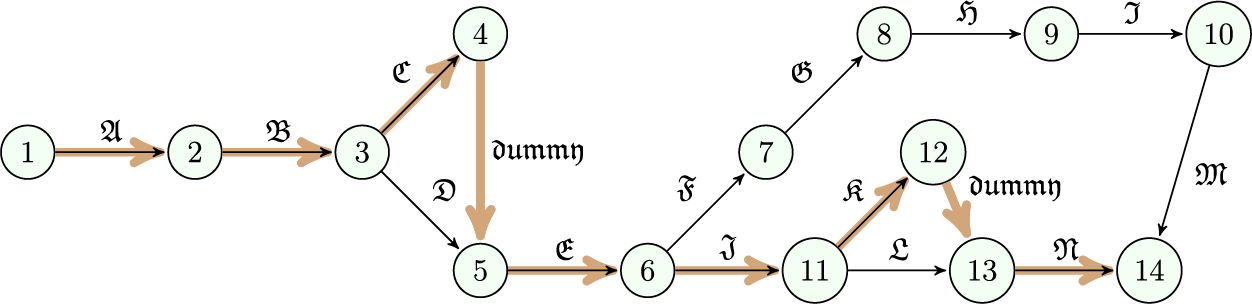
Figure 4: LDF-critical path of network diagram
Because it takes into account the parametric values, which are highly clear in real-world scenarios, together with the truth-membership and falsity-membership, the linear Diophantine fuzzy set is a generalisation of the classical set, fuzzy set, and intuitionistic fuzzy set. In this section, we have used the score function to get clear values for the PERT three-time estimations by treating them like LDF numbers. The research will be expanded in the future to cover various project management methodologies.
The Linear Diophantine fuzzy critical path method (LDF-CPM) algorithm is the generalized fuzzy critical path method based on its predicted LDF-values. In our next Sub-section 4.1, we draft the LDF-CPM algorithm followed by a flow diagram in Fig. 5 and its pseudo-code. Also in Sub-section 4.2, we draft the numerical example for the LDF-CPM.
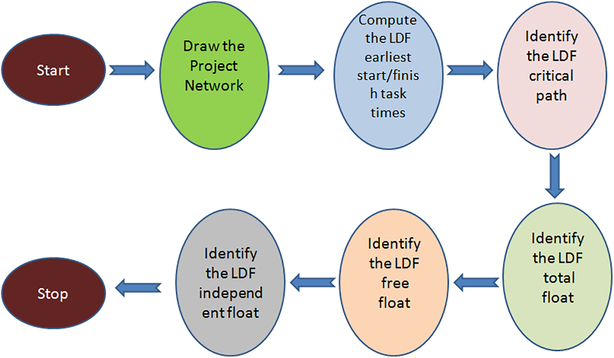
Figure 5: Flow diagram for LDF-CPM
5.1 The CPM Algorithm-Our Extension via LDFG
5.2 Case Study: Garment Production & Sales Process Problem
The garment industry is currently facing the most significant issues. PHK Industries has operated in a conventional fashion for many years and is resistant to change. They are content as long as their industry continues to thrive. They lack the confidence and motivation to replace old processes with new ones. Now is the moment to battle worldwide market requirements and specialized markets in the clothing industry. The key factors involved in this field are as follows:
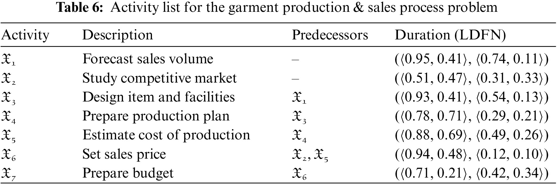
• Forecast sales volume
To plan successfully, you ought to be able to predict prospective sales with some accuracy. The majority of firms do not have firm sales projections for the future. You can, however, forecast sales based on historical data, market trends, and/or existing orders.
• Study competitive market
A way to identify competitors, and understand competitors' strengths and weaknesses in relation to ours. It helps you gauge how to curb competitors and refine your strategy to expand into a new market.
• Design items and facilities
The comfort of the user is influenced by the design of the garment. Fit is an important aspect of design to prevent impeding motion. If there are fit issues, no matter how highly designed the cloth is, it cannot be considered the best.
• Prepare a production plan
Every business needs a well-thought-out production strategy in order to optimize output. Effective planning, on the other hand, is a multi-step process that ensures that supplies, equipment, and human resources are accessible when and where they are required. Production planning functions similarly to a road map: It assists you in determining where you are heading and how long it would take to get there.
• Estimate cost of production
Costing is the process of calculating and then estimating the overall cost of creating a garment or item in the fashion industry. It often comprises costs for raw materials, garment assembly, trimmings, packing, shipping, and operational expenditures, as well as personnel.
• Set sales price
Now that the items are in stock, you must sell them. Selling has a number of expenses that will eat into your profit margin. It is critical to understand the difference between wholesale and retail prices. The wholesale pricing is lower, which means you’ll have a smaller profit margin but cheaper costs. We have more control over the ultimate retail price and the margin you make when you sell directly to customers, but you must account for additional risks, such as stock risk, and expenditures, such as marketing costs, location store charges, and so on.
• Prepare budget
Budget preparation is the main, essential and final task of the project.
In this part of the paper, we are going to solve the problem of this garment problem using the linear Diophantine fuzzy critical path method (LDF-CPM). The LDF-Critical path of the network diagram is given in Fig. 6. Activity list for the garment production & sales process problem is listed in Table 6.
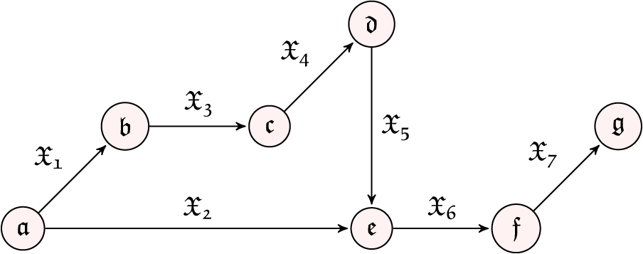
Figure 6: LDF-critical path of network diagram
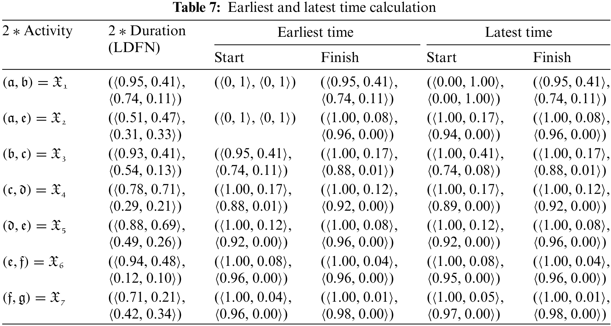
5.2.1 Linear Diophantine Fuzzy Earliest Start Task Times
•
•
•
•
•
•
•
5.2.2 Linear Diophantine Fuzzy Latest Finishing Task Times
• Let
•
•
•
•
•
•
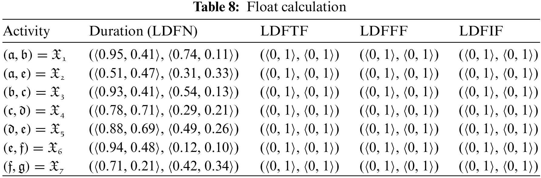
5.2.3 Results and Discussion for Garment Production & Sales Process Problem
From Sections 5.2.1 and 5.2.2, we conclude that the linear Diophantine fuzzy critical path is
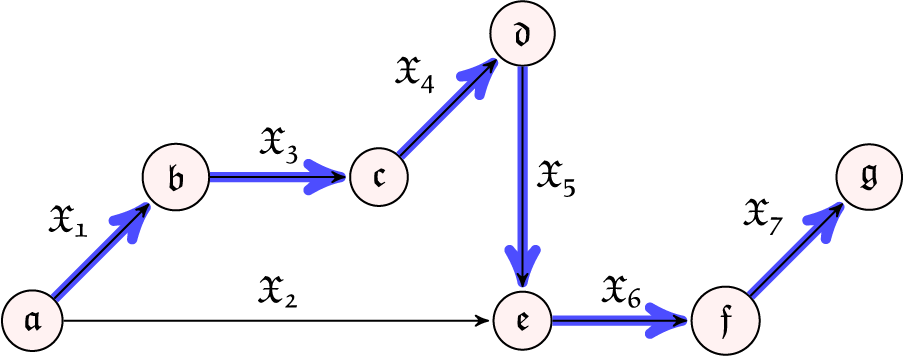
Figure 7: LDF-critical path of network diagram
When uncertainty arises during various activities like planning, scheduling, developing, designing, testing, maintaining, and advertising for the fields of administration, construction, manufacturing, and marketing, etc., this method is much more helpful than other existing methods like CPM/PERT, fuzzy CPM/PERT, and intuitionistic fuzzy CPM/PERT, etc.
(i) It provides superior accuracy in every single project activity than other methods.
(ii) Because of its precision, it is simple to identify the ideal timeline for any project.
(iii) By linking them, the degree of performance for every task will also be raised.
(iv) It becomes very easy to control each action in a project.
1. Accuracy and supremacy: Proposed LDFS PERT/CPM frameworks are adequate and applicable for a range of input data sources. The methods demonstrate great accuracy in comparison to previous approaches and are capable of handling uncertainties and ambiguities as well as correcting flaws in the supplied data. The LDFS, which are hybrid structured sets, can be used to gather data against several alternatives on a big scale.
2. Managing several criteria with efficiency: Decision support system challenges entail a variety of criteria and input data that vary depending on the scenario. The LDFS proposed are simple and clear, allowing for their seamless use in any circumstance including several choices and criteria.
3. Superiority and flexibility: Proposed LDFS PERT/CPM algorithms are distinguished by their simplicity, adaptability, and superiority in comparison to other hybrid fuzzy sets and operators. Its high adaptability permits administrators to conduct comparative analysis at multiple levels, resulting in solutions that are more optimal. As a consequence of this research, a method for selecting the optimal algorithm from a list of algorithms has been developed. Our proposed method is less sensitive to input and output data variations, making it a valuable tool for managers who must evaluate options in the face of high levels of uncertainty and ambiguity.
In this study, we have proposed a novel analytical approach for determining the critical path in an LDF project network. Our method utilizes a defuzzification approach for LD fuzzy numbers, employing scoring functions and accuracy functions. We have applied this approach to calculate the float time for each activity in the LDF project network. The results indicate that LDF models are highly effective in detecting critical paths, especially in real project network anomalies. We have employed the LDF-PERT and LDF-CPM representation procedures (algorithms) to determine the optimal path in a linear Diophantine fuzzy weighted setting. This provides valuable assistance to decision-makers in identifying the best critical path in LD fuzzy settings. Moreover, our novel techniques are relatively easy to implement and yield minimum LDF-CPM/LDF-PERT with a reduced number of dummy arcs. It is worth noting that the techniques used in the seven rules of the algorithm can be applied in other disciplines by specialists in graph theory. Additionally, the experimental results demonstrate the effectiveness of our method, even for large-scale networks. Another significant advantage is that our approach works seamlessly in the presence of transitive arcs. In future research, we plan to extend the application of these LDF-CPM/LDF-PERT techniques to other network models. Furthermore, we aim to develop software to better implement the information measures derived from this study in practical scenarios. Future studies should also explore various ranking systems, determine the Critical Degree (CD) for locating the Critical Path, and apply the method to address real-world Project Management issues. Additionally, LDFSs can be examined from the perspectives of cost analysis, earned value analysis, and resource-constrained project scheduling. These areas provide promising avenues for further investigation and application of LDFSs in Project Management.
Acknowledgement: This work was supported by the Deanship of Scientific Research, Vice Presidency for Graduate Studies and Scientific Research, King Faisal University, Saudi Arabia [Grant No.GRANT3862].
Funding Statement: King Faisal University Research Grant GRANT3862.
Author Contributions: All authors contributed equally to this paper. The individual responsibilities and contributions of all authors can be described as follows: M. Parimala., K. Parkash., and S. Jafari. contributed on methodology, formal analysis, write up original draft. M. Riaz., and A. Al-Quran. both contributed on conceptualizations, methodology, investigations.
Availability of Data and Materials: No data and no material were used in this study.
Conflicts of Interest: The authors declare that they have no conflicts of interest to report regarding the present study.
References
1. Badiru, A. B., Osisanya, S. O. (2016). Project management for the oil and gas industry: A world system approach. Boca Raton, FL, USA: CRC Press. [Google Scholar]
2. Haga, W. A., O’Keefe, T. (2001). Crashing PERT networks: A simulation approach. 4th International Conference of the Academy of Business and Administrative Sciences Conference, Quebec City, Canada. [Google Scholar]
3. Campos, S. M., Fierro, T. E., Solis, A. P., Saltillo, C. M., Saltillo, C. M. et al. (2003). Modeling an assembly line combining PERT/CPM to study the flexibility of a mexican automotive plant using simulink. Proceedings of the 8th Annual International Conference on Industrial Engineering-Theory, Applications and Practice, Las Vegas, Nevada, USA. [Google Scholar]
4. Zadeh, L. A. (1965). Fuzzy sets. Information and Control, 8, 338–353. [Google Scholar]
5. Elizabeth, S., Sujatha, L. (2013). Fuzzy critical path problem for project network. International Journal of Pure and Applied Mathematics, 85(2), 223–240. [Google Scholar]
6. Chen, C. T., Huang, S. F. (2007). Applying fuzzy method for measuring criticality in project network. Information Sciences, 177(12), 2448–2458. [Google Scholar]
7. Dubois, D., Prade, H. (2012). Possibility theory: An approach to computerized processing of uncertainty. Berlin/Heidelberg, Germany: Springer Science Business Media. [Google Scholar]
8. Hapke, M., Slowinski, R. (1996). Fuzzy priority heuristics for project scheduling. Fuzzy Sets and Systems, 83(3), 291–299. [Google Scholar]
9. Chen, S. M., Chang, T. H. (2001). Finding multiple possible critical paths using fuzzy PERT. IEEE Transactions on Systems, Man, and Cybernetics—Part B (Cybernetics), 31(6), 930–937. [Google Scholar]
10. Yao, J. S., Lin, F. T. (2000). Fuzzy critical path method based on signed distance ranking of fuzzy numbers. IEEE Transactions on Systems, Man, and Cybernetics—Part A: Systems and Humans, 30(1), 76–82. [Google Scholar]
11. Cheng, F., Lin, M., Yuksel, S., Dincer, H., Kalkavan, H. (2020). A hybrid hesitant 2-tuple IVSF decision making approach to analyze PERT-based critical paths of new service development process for renewable energy investment projects. IEEE Access, 9, 3947–3969. [Google Scholar]
12. Habibi, F., Birgani, O., Koppelaar, H., Radenovic, S. (2018). Using fuzzy logic to improve the project time and cost estimation based on project evaluation and review technique (PERT). Journal of Project Management, 3(4), 183–196. [Google Scholar]
13. Ballesteros-Perez, P. (2017). M-PERT: Manual project-duration estimation technique for teaching scheduling basics. Journal of Construction Engineering and Management, 143(9), 04017063. [Google Scholar]
14. Miralles-Pechuan, L., Rosso, D., Jimenez, F., Garcia, J. M. (2017). A methodology based on deep learning for advert value calculation in CPM, CPC and CPA networks. Soft Computing, 21(3), 651–665. [Google Scholar]
15. Hu, C., Liu, D. (2018). Improved critical path method with trapezoidal fuzzy activity durations. Journal of Construction Engineering and Management, 144(9), 04018090. [Google Scholar]
16. Takakura, Y., Yajima, T., Kawajiri, Y., Hashizume, S. (2019). Application of critical path method to stochastic processes with historical operation data. Chemical Engineering Research and Design, 149, 195–208. [Google Scholar]
17. Kusumadarma, I. A., Pratami, D., Yasa, I. P., Tripiawan, W. (2020). Developing project schedule in telecommunication projects using critical path method (CPM). International Journal of Integrated Engineering, 12(3), 60–67. [Google Scholar]
18. Kim, K. (2020). Generalized resource-constrained critical path method to improve sustainability in construction project scheduling. Sustainability, 12(21), 8918. [Google Scholar]
19. Ba’Its, H. A., Puspita, I. A., Bay, A. F. (2020). Combination of program evaluation and review technique (PERT) and critical path method (CPM) for project schedule development. International Journal of Integrated Engineering, 12(3), 68–75. [Google Scholar]
20. Liu, D., Hu, C. (2021). A dynamic critical path method for project scheduling based on a generalised fuzzy similarity. Journal of the Operational Research Society, 72(2), 458–470. [Google Scholar]
21. Khalifa, H. A. E. W., Alharbi, M. G., Kumar, P. (2021). On determining the critical path of activity network with normalized heptagonal fuzzy data. Wireless Communications and Mobile Computing, 2021, 6699403. [Google Scholar]
22. Yogashanthi, T., Prabakaran, K., Ganesan, K. (2021). Application of intuitionistic fuzzy critical path method on airfreight ground operation systems. Journal of Mathematical and Computational Science, 11(4), 4518–4534. [Google Scholar]
23. Yudiarti, W. W., Razi, F. A. (2021). Application of critical path method and fuzzy logic in optimizing bottled drinking water production. InPrime: Indonesian Journal of Pure and Applied Mathematics, 3(1), 53–62. [Google Scholar]
24. Yang, J. Q., Chen, C. H., Li, J. Y., Liu, D., Li, T. et al. (2022). Compressed-encoding particle swarm optimization with fuzzy learning for large-scale feature selection. Symmetry, 14(6), 1142. https://doi.org/10.3390/sym14061142 [Google Scholar] [CrossRef]
25. Tang, Y., Pan, Z., Pedrycz, W., Ren, F., Song, X. (2022). Viewpoint-based kernel fuzzy clustering with weight information granules. IEEE Transactions on Emerging Topics in Computational Intelligence. https://doi.org/10.1109/TETCI.2022.3201620 [Google Scholar] [CrossRef]
26. Atanassov, K. T. (1986). Intuitionistic fuzzy sets. Fuzzy Sets and Systems, 20(1), 87–96. [Google Scholar]
27. Atanassov, K. T. (1999). Interval valued intuitionistic fuzzy sets. In: Intuitionistic fuzzy sets, pp. 139–177. Heidelberg: Physica. [Google Scholar]
28. Jayagowri, P., Geetharamani, G. (2014). A critical path problem using intuitionistic triangular fuzzy number. International Journal of Engineering Research and Applications, 4(5), 55–60. [Google Scholar]
29. Kiruthiga, M., Hemalatha, T. (2019). Intuitionistic fuzzy technique to find the critical path. International Journal of Statistics and Applied Mathematics, 4(3), 39–42. [Google Scholar]
30. Yager, R. R. (2013). Pythagorean fuzzy subsets. 2013 Joint IFSA World Congress and NAFIPS Annual Meeting (IFSA/NAFIPS), pp. 57–61. Edmonton, AB, Canada. [Google Scholar]
31. Yager, R. R., Abbasov, A. M. (2013). Pythagorean membership grades, complex numbers, and decision making. International Journal of Intelligent Systems, 28, 436–452. [Google Scholar]
32. Yager, R. R. (2013). Pythagorean membership grades in multicriteria decision making. IEEE Transactions on Fuzzy Systems, 22(4), 958–965. [Google Scholar]
33. Riaz, M., Hashmi, M. R. (2019). Linear Diophantine fuzzy set and its applications towards multi-attribute decision-making problems. Journal of Intelligent & Fuzzy Systems, 37(4), 5417–5439. [Google Scholar]
34. Riaz, M., Hashmi, M. R., Kalsoom, H., Pamucar, D., Chu, Y. M. (2020). Linear Diophantine fuzzy soft rough sets for the selection of sustainable material handling equipment. Symmetry, 12(8), 1215. [Google Scholar]
35. Riaz, M., Farid, H. M. A. (2023). Multi-criteria decision-making algorithm based on linear Diophantine fuzzy aggregation operators. Journal of Multiple-Valued Logic & Soft Computing, 40, 221–251. [Google Scholar]
36. Parimala, M., Jafari, S., Riaz, M., Aslam, M. (2021). Applying the Dijkstra algorithm to solve a linear Diophantine fuzzy environment. Symmetry, 13(9), 1616. [Google Scholar]
37. Iampan, A., Garcia, G. S., Riaz, M., Athar Farid, H. M., Chinram, R. (2021). Linear Diophantine fuzzy Einstein aggregation operators for multi-criteria decision-making problems. Journal of Mathematics, 2021, 5548033. [Google Scholar]
38. Alshammari, I., Parimala, M., Ozel, C., Riaz, M., Kammoun, R. (2022). New MCDM algorithms with linear Diophantine fuzzy soft TOPSIS, VIKOR and aggregation operators. Mathematics, 10(17), 3080. [Google Scholar]
39. Almagrabi, A. O., Abdullah, S., Shams, M., Al-Otaibi, Y. D., Ashraf, S. (2022). A new approach to q-linear Diophantine fuzzy emergency decision support system for COVID-19. Journal of Ambient Intelligence and Humanized Computing, 13(4), 1687–1713. [Google Scholar] [PubMed]
40. Kamaci, H. (2022). Complex linear Diophantine fuzzy sets and their cosine similarity measures with applications. Complex & Intelligent Systems, 8(2), 1281–1305. [Google Scholar]
41. Karabulut, M. (2017). Application of Monte Carlo simulation and PERT/CPM techniques in planning of construction projects: A case study. Periodicals of Engineering and Natural Sciences (PEN), 5(3), 408–420 [Google Scholar]
42. Musarandega, R., Robinson, J., Sen, P. D., Hakobyan, A., Mushavi, A. et al. (2020). Using the critical path method to rollout and optimise new PMTCT guidelines to eliminate mother-to-child transmission of HIV in Zimbabwe: A descriptive analysis. BMC Health Services Research, 20(1), 1–11. [Google Scholar]
43. Akram, M., Khan, A., Alcantud, J. C. R., Santos-Garcia, G. (2021). A hybrid decision-making framework under complex spherical fuzzy prioritized weighted aggregation operators. Expert Systems, 38(6), 1–24. [Google Scholar]
44. Feng, F., Zheng, Y., Sun, B., Akram, M. (2022). Novel score functions of generalized orthopair fuzzy membership grades with application to multiple attribute decision making. Granular Computing, 7(1), 95–111. [Google Scholar]
45. Hanif, M. Z., Yaqoob, N., Riaz, M., Aslam, M. (2022). Linear Diophantine fuzzy graphs with new decision-making approach. AIMS Mathematics, 7(8), 14532–14556. [Google Scholar]
46. Pamucar, D. (2020). Normalized weighted geometric Dombi Bonferroni mean operator with interval grey numbers: Application in multicriteria decision making. Reports in Mechanical Engineering, 1(1), 44–52. [Google Scholar]
47. Riaz, M., Farid, H. M. A. (2023). Enhancing green supply chain efficiency through linear Diophantine fuzzy soft-max aggregation operators. Journal of Industrial Intelligence, 1(1), 8–29. [Google Scholar]
48. Dordevic, M., Tesic, R., Todorovic, S., Jokic, M., Das, D. K. et al. (2022). Development of integrated linear programming fuzzy-rough MCDM model for production optimization. Axioms, 11(10), 510. [Google Scholar]
49. Ali, Z., Mahmood, T., Ullah, K., Khan, Q. (2021). Einstein geometric aggregation operators using a novel complex interval-valued Pythagorean fuzzy setting with application in green supplier chain management. Reports in Mechanical Engineering, 2(1), 105–134. [Google Scholar]
50. Al-Quran, A. (2023). T-spherical linear Diophantine fuzzy aggregation operators for multiple attribute decision-making. AIMS Mathematics, 8(5), 12257–12286. [Google Scholar]
51. Al-Sharqi, F., Ahmad, A., Al-Quran, A. (2022). Fuzzy parameterized-interval complex neutrosophic soft sets and their applications under uncertainty. Journal of Intelligent and Fuzzy Systems, 44(1), 1–25. [Google Scholar]
52. Al-Quran, A. (2021). A new multi attribute decision making method based on the T-spherical hesitant fuzzy sets. IEEE Access, 9, 156200–156210. [Google Scholar]
53. Riaz, M., Riaz, M., Jamil, N., Zararsiz, Z. (2022). Distance and similarity measures for bipolar fuzzy soft sets with application to pharmaceutical logistics and supply chain management. Journal of Intelligent & Fuzzy Systems, 42(4), 3169–3188. [Google Scholar]
54. Zararsiz, Z. (2016). On the extensions of the almost convergence idea and core theorems. Journal of Nonlinear Science with Applications, 9, 112–125. [Google Scholar]
55. Sezgin, A., Atagun, A. O., Cagman, N., Demir, H. (2022). On near-rings with soft union ideals and applications. New Mathematics and Natural Computation, 18(2), 495–511. [Google Scholar]
56. Atagun, A. O., Kamaci, H., Tastekin, I., Sezgin, A. (2019). P-properties in near-rings. Journal of Mathematical and Fundamental Sciences, 51(2), 152–167. [Google Scholar]
57. Habib, A., Khan, Z. A., Riaz, M., Marinkovic, D. (2023). Performance evaluation of healthcare supply chain in Industry 4.0 with linear Diophantine fuzzy sine-trigonometric aggregation operations. Mathematics, 11(12), 2611. [Google Scholar]
58. Bozanic, D., Pamucar, D., Badi, I., Tesic, D. (2023). A decision support tool for oil spill response strategy selection: Application of LBWA and Z MABAC methods. Opsearch, 60(1), 24–58. [Google Scholar]
Cite This Article
 Copyright © 2024 The Author(s). Published by Tech Science Press.
This work is licensed under a Creative Commons Attribution 4.0 International License , which permits unrestricted use, distribution, and reproduction in any medium, provided the original work is properly cited.
 Downloads
 Citation Tools