CALTM: A Context-Aware Long-Term Time-Series Forecasting Model

1  Introduction

With remarkable economic advancements and rising living standards in recent years, there has been a notable surge in the preference for automobile travel, engendering a surge in highway traffic volume during holidays and leading to heightened congestion. At present, the handling of highway congestion problems usually relies on appropriate traffic control measures, such as vehicle restrictions, closure of the highway gate. And these common control measures usually need to be formulated in conjunction with the forecast results of traffic volume in order to achieve better results. Therefore, accurately forecasting traffic volume during holidays and implementing effective control measures are crucial for managing highway congestion and ensuring smooth operations. However, the complexity of transportation networks and the dynamic nature of traffic volume pose significant challenges in real-world scenarios.

Existing traffic volume forecasting methods encompass short-term and trend forecasting, with the former being mainstream. Short-term forecasting techniques can be categorized into mainstream time series forecasting and deep learning-based forecasting. Mainstream time series forecasting methods often rely on statistical models, such as the Autoregressive Integrated Moving Average model (ARIMA) [1], Kalman filter utilizing seasonal traffic volume data [2], SVM combined with a denoising algorithm [3], and state vector combined with K-nearest neighbors (KNN) method [4]. In recent years, deep learning models have gained prominence in traffic volume forecasting owing to their generalization capabilities and adeptness in capturing subtle changes. Deep Belief Networks (DBN) with a probabilistic directed graph model [5] leverage a multi-layer node graph structure to capture time-space correlations and extract effective features from traffic data. Recurrent Neural Network (RNN) structures [6], including Long Short-Term Memory (LSTM) [7], Gated Recurrent Unit (GRU) [7,8], and other sequence-based deep learning models, learn temporal dependencies through contextual analysis of sequences. Additionally, the Temporal Convolutional Network (TCN) [9] captures the spatiotemporal evolution of traffic volume through convolutional neural networks. However, these methods struggle to fully analyze the correlation of traffic volume across different roads and extract dynamic characteristics, leading to suboptimal forecasting accuracy.

Recent research has improved forecasting accuracy by incorporating spatial factors, such as Graph Convolutional Networks (GCN) [10] model, which aggregates neighboring nodes’ information through graph embedding techniques, then uses convolution to extract features that capture dynamic traffic data and spatiotemporal variation dependency. T-GCN [11], AST-GCN-LSTM model [12,13] incorporate GCN and GRU for capturing spatial and temporal dependencies, respectively, improving the traditional combination of RNN and GCN for spatiotemporal traffic volume forecasting. The Spatio-Temporal Graph Convolutional Network (ST-GCN) model with a spatial-graph attention mechanism [14] is used for traffic volume forecasting. Finally, a knowledge-graph fusion cell (KF-Cell) [15] that combines knowledge and volume features were added to the spatiotemporal graph convolution network to improve performance in different forecasting ranges. HetGAT [16] utilizes a weighted graph attention network (GAT) to encode the input temporal features and to decode the output velocity sequence through the express network structure. Although the above methods use the traffic network topology combined with the deep learning model to obtain good traffic volume forecasting results, they only focus on short-term forecasting scenarios and only consider the recent traffic volume information. This paper focuses on holiday traffic volume forecasting, which requires considering the characteristics of different holidays and recent traffic conditions. Moreover, as holiday traffic forecasting belongs to trend forecasting, it cannot rely on short-term historical data, and effective features need to be mined from long-term historical data. In rare trend forecasting methods, Li et al. [17] decomposed the original traffic volume data into three periods: long, medium, and short, and processed them separately. They integrated the predicted results of the three deep learning models to make long-term forecastings of traffic volume. However, the time series decomposition of this method requires the datasets to have strong periodicity and rely on short-term historical traffic volume data. Obviously, more than the generality of this method is needed, it is unsuitable for holiday traffic datasets with significant fluctuations, and it cannot mine adequate information from complex and changeable historical data sets.

With the goal of addressing the above issues, we propose a holiday traffic volume forecasting model called CALTM (Context-Aware Long-Term Time-Series Forecasting Model) based on long and short-term scene representation fusion. The model consists of three parts: the similar scene matching module (S2M2), the long-short term representation fusion module, and the head of a simple full connection layer. Among them, the similar scene matching module is applicable to all time series problems with rich context features, and is a plug-and-play module that can find series with similar scenes to the series to be predicted from the historical data set. In order to comprehensively consider various influencing factors of holiday traffic volume, the model finds historical traffic volume with similar scenes through the similar scene matching module, then combines recent traffic volume data, similar historical traffic volume data and “time, weather, epidemic control, and tolls” conditions using the long-short term representation fusion module for holiday forecasting. The model uses a multi-head attention mechanism and context feature encoder to fuse multiple related features and fully utilize the information in the text to improve the accuracy of the model’s forecastings. Extensive experiments on a real etc dataset demonstrate that CALTM sets a new state-of-the-art performance. Especially, compared with N-BEATS [18], CALTM reduces the MSE 27.2%, 12.0%, 26.3%, and 7.7% on the four datasets H7, W7, H3, and W3, respectively.

In conclusion, our contributions are summarized as follows:

•   We propose a novel plug-in module, S2M2, that can be applied to all time series problems with rich contextual features to identify similar historical time series. It is a multi-dimensional method and performs effective embedding, which can adapt to the effective encoding method of special scenes such as weekends and holidays.

•   For the purpose of addressing the challenge of insufficient long-term sequence forecast capability in recurrent neural networks, we propose CALTM, a holiday traffic volume forecasting model framework that combines scene and sequential context.

•   We use the volume data of expressway toll stations in Zhejiang Province to verify the validity of traffic volume forecast on statutory holidays (Qingming, May Day, Dragon Boat Festival, etc.) and ordinary weekends. The experimental results demonstrate that our model has improved compared with the mainstream statistical model, recurrent neural network model, convolutional network for mining time series features.

2  Problem Formulation

Definition 1: A collection of toll/section flow sequences. Among them, section refers to the branch roads that converge on the main highway. Let seq denote a toll/section flow sequence, representing the highway traffic volume sequence <v1,v2,…,vStep> at a given time step Step. Let S represent the set of all toll/section flow sequences for a given time instance T. Thus, we have seq ∈ S.

Definition 2: Representation of contextual traffic factors. The contextual features such as “time, weather, epidemic situation, and toll or free access of the highway” in the dataset are mapped to vector representations via embeddings, and concatenated to obtain a context representation through a Contextual Feature Encoder (MLP). The context representation is denoted by hc (Formal representation: tuple).

Definition 3: Collection of similar toll/section flow sequences. Given the collection of toll/section flow sequences S, the top-k sequences are selected to form a collection of similar sequences denoted by Ssim=seq1,seq2,…,seqk using a similarity sequence retrieval algorithm applied on the sequences in S.

Definition 4: Traffic representation with attention interaction. Given a sequence of observed traffic volume seqobserved to be predicted and the collection of similar toll/section flow sequences Ssim, an attention interaction module is used to fuse them together and obtain a traffic representation with attention interaction denoted by hsim. Among them, the seqobserved is the traffic flows from Tahead+k days to Tahead+1 before the holiday to be predicted. And Tahead denotes we will predict holidays after Tahead days.

Definition 5: The input of the CALTM model includes four parts: toll similar traffic flow sequence seqsim,toll, cross-sectional similar traffic flow sequence seqsim,section, observed traffic flow sequence seqobserved, and four contextual features: time, wea, epi, and fee. Among the four contextual features, time represents the date type, wea represents weather, epi represents epidemic control and fee represents whether the highway is free.

Problem Definition: Given a collection of toll/section flow sequences S and the context representation hc, the objective is to traverse the collection S from Tahead+k backwards in time to obtain similar toll/section flow sequences seqsim,toll and seqsim,sec. These sequences, along with hc and the observed traffic volume sequence seqobserved, are then used as input to the model for predicting the holiday traffic volume sequence seqt at a given time instance Tt with time step Stept.

3  Methodology

In this section, we present our Context-Aware Long-Term Time-Series Forecasting Model termed as CALTM, as shown in Fig. 1. The proposed framework contains three components, i.e., the similar scene matching module for Similar Scene Mining, the long-short term representation fusion module for mixing scenario cues, and the head of a simple fully connection layer for flow forecasting. In the following sections, we first describe the specific details of the similar scene matching module, then elaborate on the concrete construction of long-short term representation fusion, which consists of three main components: the recurrent neural network encoder, the attention interaction, and the contextual representation.

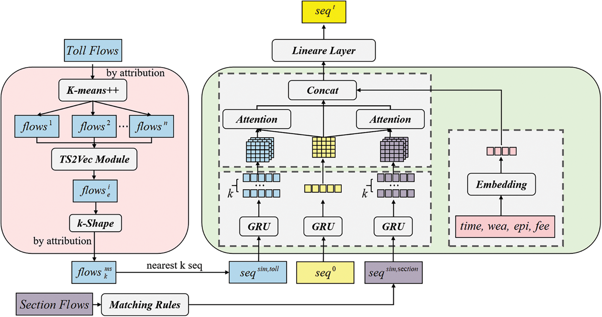
Figure 1: The overall view of CALTM framework

3.1 Similar Scene Matching Module (S2M2)

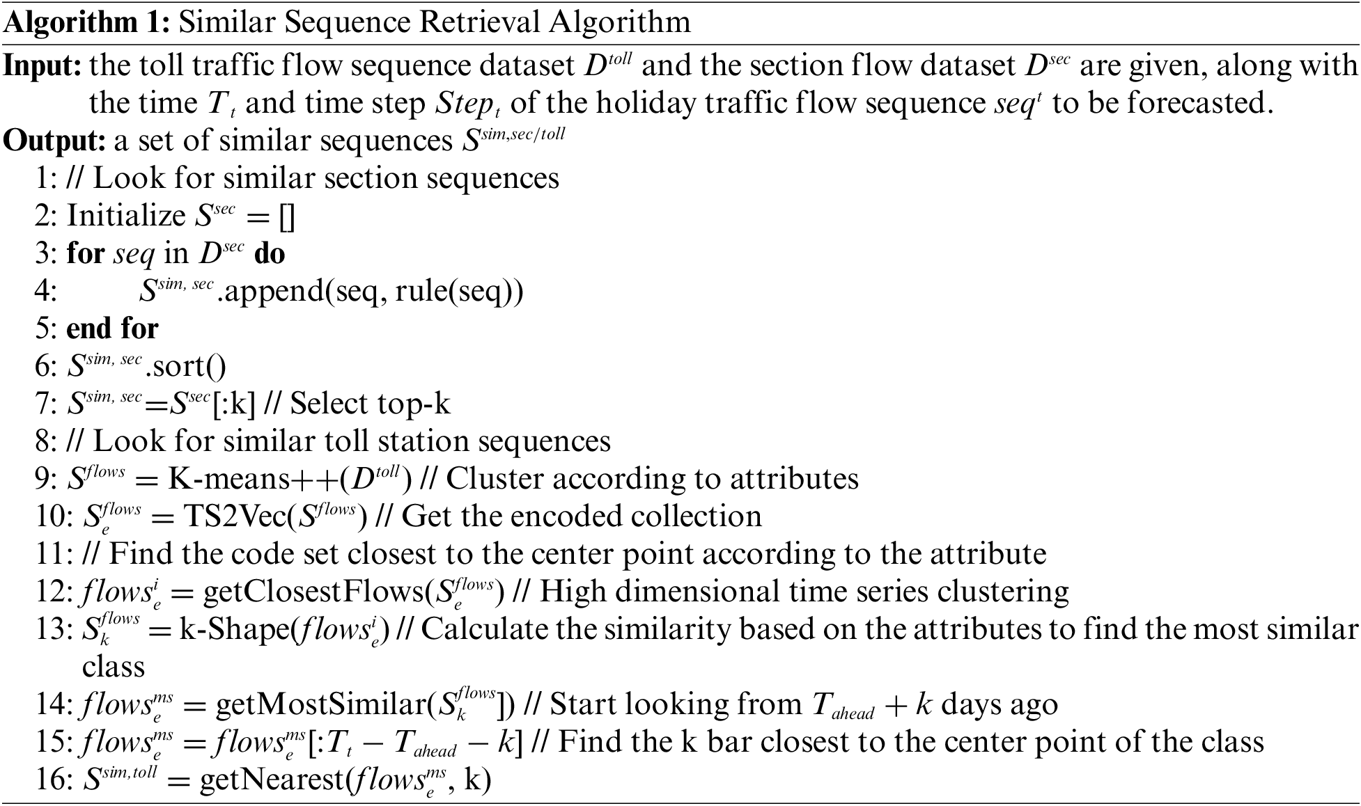
The similar scene matching module (S2M2), depicted in the left part of Fig. 1, is the core design to mine the time series context. It aims to identify historical time series with similar characteristics to a given time series. Since holiday traffic forecasting falls under long-term forecasting, it is necessary to retrieve sequences of equal length that are similar to the external information of the sequence being forecasted. For main/tollgate sequences, contrastive learning is performed hierarchically on an enhanced context view using TS2Vec, increasing the distance between historical time series with different attributes. Furthermore, using the k-Shape clustering algorithm to cluster the encoded embeddings is beneficial for us to obtain the historical traffic flow sequence of the scene similar to the sequence to be forecasted according to the similarity of attributes. Finally, by searching for the category with the highest attribute similarity, the time series closest to the center point of that category are obtained as similar sequences. Aiming to handle traffic sequences lacking context features, specific rules are defined to identify similar sequences. In this paper, for the section volume sequences, the sequences of similar dates in previous years of the same section are considered as similar sequences. It is worth noting that our general-purpose method, S2M2, can be applied to all time series problems with rich contextual features. The whole algorithm is summarized with pseudocode in Algorithm 1. We give a detailed explanation as follows.

3.1.1 Cluster Series Scenarios

The toll traffic sequence data is clustered according to the three attributes of holidays (hol), weather (wea), and epidemic situation (epi). Determine the optimal number of clusters n using the elbow method, and obtain clustering results Sflows={flows1,flows2,...,flowsn}, where the n represents the number of clusters, flowsi={seq1toll,seq2toll,...,seqxtoll}, and x represents the total number of traffic sequences in each cluster.

3.1.2 Encode Series via TS2Vec

TS2Vec [19] improves the robustness of features in the input time series collection through timestamp masking and random cropping. Then, instance-wise and temporal contrastive losses are combined to capture contextual representations of time series. The two losses complement each other, with instance contrast learning user-specific characteristics and temporal contrast mining dynamic trends over time. The specific encoding process of TS2Vec is shown in Fig. 2. And the main role of TS2Vec in this article is to expand the differences between traffic flow sequences with different temporal features, in order to achieve better clustering results in the future. Therefore, the role of TS2Vec can be understood as expanding the distance between positive and negative samples, in order to better extract useful features.

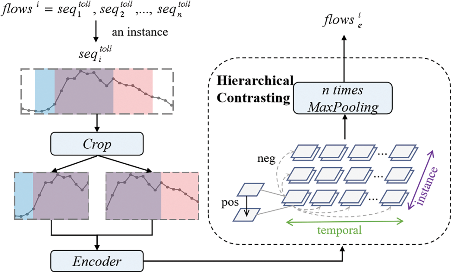
Figure 2: Comparative learning framework

In order to learn discriminative representations over time, TS2Vec employs a Temporal Contrastive Loss. This loss considers the representations of the same timestamp from two views of the input time series as positives, while treating those at different timestamps from the same time series as negatives. Let i denotes the index of the input time series sample and t denote the timestamp. The representations for the same timestamp t but from two augmentations of xi are denoted as ri,t and ri,t′. The temporal contrastive loss for the i-th time series at timestamp t is then formulated as

ℓtemp(i,t)=−logexp(ri,t⋅ri,t′)∑t′∈Ω(exp(ri,t⋅ri,t′′)+Lt≠t′exp(ri,t⋅ri,t′)(1)

where Ω is the set of timestamps within the overlap of the two subseries, and L is the indicator function.

The instance-wise contrastive loss indexed with (i,t) can be formulated as

ℓinst(i,t)=−logexp(ri,t⋅ri,t′)∑j=1B(exp(ri,t⋅rj,t′)+Li≠jexp(ri,t⋅rj,t)(2)

where B denotes the batch size. We use representations of other time series at timestamp t in the same batch as negative samples.

The two types of losses complement each other. For instance, when dealing with a collection of electricity consumption data that pertains to different users, the instance contrast loss can capture the user-specific patterns, while the temporal contrast loss focuses on capturing the evolving trends over time. The complete loss function is defined as follows:

ℒdual=1NT∑i∑t(ℓtemp(i,t)+ℓinst(i,t))(3)

where N is the number of time series, and T is the length of each time series, therefor NT is the sum of the lengths of all time series.

3.1.3 Extract Discriminative Feature of Series

Suppose the attributes for holidays, weather, and episodes during a given time period are represented as holt,weat,epit, and flowsi have their respective centroids as holi,weai,epii. Calculate the distance between each category’s centroid and Sflows using the formula for Euclidean distance to find the closest category, which is denoted as flowsei. The distance is defined by the following formula:

distance=(holt−holi)2+(weat−weai)2+(epit−epii)2(4)

First, k-Shape clustering is applied to flowsei, and the optimal number of clusters m is determined using the elbow method. Subsequently, Skflows={flowsk1,flowsk2,…,flowskm} are obtained, where each flowski is composed of {seq1(toll,k),seq2(toll,k),…,seqy(toll,k)}, with y representing the total number of traffic flow sequences in the cluster.

3.1.4 Measure Similarity of Series

Based on the attributes of holidays (holt), weather (weat), and epidemic (epit), their average distance to the attribute sets of various time series in Skflows is calculated to measure attribute similarity. The category flowsems with the highest similarity (i.e., the shortest distance) is obtained. It is assumed that the attribute of a traffic flow sequence seqi1(toll,k) in flowski is holi1,weai1,epii1, and the average distance can be represented as follows:

distanceavg=1y∑i1=1y((holt−holi1)2+(weat−weai1)2+(epit−epii1)2)(5)

Subsequently, we filtered the traffic sequences in flowsems and retained only the traffic sequences for the previous Tahead+k days during holidays and weekends. We then selected k traffic sequences that had the closest Euclidean distance to the center point and defined them as the set of toll traffic similar sequences Stoll={seq1sim,toll,seq2sim,toll,…,seqksim,toll}∈RK×Stept×1, where seqsim,toll=<v1,v2,…,vStept>∈RStept×1.

3.1.5 Define the Ranking Rule

For cross-sectional flow rate, due to the lack of contextual features in the etc dataset of G25-G50 expressway (only time is available), and the time period is from June 2020 to June 2021, which corresponds to historical periods of holidays and festivals, a matching rule was used to identify similar sequences. If the observed date falls on a weekend, the cross-sectional flow rate sequence dataset Dsec is filtered to retain the data for weekends and select the k most recent data. If the observed date is a legal holiday, historical holiday data from the same period is selected. If there are less than k data available, the most recent legal holiday data is used as a supplement to obtain a set of similar sequences Ssec=seq1sim,sec,seq2sim,sec,…,seqksim,sec∈RK×Stept×1, where seqsim,sec=<v1,v2,…,vStept>∈RStept×1.

3.2 Long-Short Term Representation Fusion Module

The long-short term representation fusion module, depicted on the right side of Fig. 1, which contains three components: the recurrent neural network encoder, the attention interaction, and the contextual representation. The input of the recurrent neural network encoder is mainly composed of three types of traffic volume sequences: the toll station volume sequence, section volume sequence, and recent holiday volume sequence to be forecasted. The volume sequence before the forecasted holiday is used as the query, and the encoding results of k toll station sequences provided by similar scene matching modules are used as key and value. The attention module employs MultiheadAttention(Q,K,V) to obtain the toll station attention interaction representation. Similarly, the volume sequence before the forecasted holiday is used as the query, and the encoding results of k sections are used as key and value. MultiheadAttention(Q,K,V) is applied to obtain the section attention interaction representation. Then the contextual feature encoding module includes categorical variables such as time, weather, pandemic situation, and whether the highway is toll-free which represent contextual features. They are mapped to vector representations through an embedding layer and concatenated before being input to the contextual feature encoder (MLP) to obtain the contextual representation. Finally, the output representation of the attention interaction module and the contextual representation are concatenated and fed to an MLP for feature fusion, then through a linear layer, the medium and long-term holiday traffic forecasting results are obtained.

3.2.1 Recurrent Neural Network Encoder

This module is designed to encode three types of flow sequences, including K similar traffic sequences Stoll on the main line, recent holiday traffic sequences seqobserved=<v1,v2,…,vStepo>∈RStepo×1 to be forecasted, and K similar traffic sequences Ssec at cross sections, in order to obtain their respective representations.

Input the three types of flow sequences, Stoll, seqobserved, and Ssec, separately into the gated recurrent neural network gate recurrent Unit (GRU) to learn the corresponding representations Etoll={h1sim,toll,h2sim,toll,…,hksim,toll}, hobserved, and Esec={h1sim,sec,h2sim,sec,…,hksim,sec}. The formulae are as follows:

ri=σ(Wr⋅[hi−1,seqi])(6)

hi~=σ(Wo⋅[ri⊙hi−1,seqi]+bo)(7)

zi=σ(Wz⋅[hi−1,seqi])(8)

hi=(1−zi)⊙hi−1+zi⊙hi^(9)

where seqi represents the input at each time step, hi−1 represents the output value of the previous unit, and hi can be regarded as a mixture of the unit state and hidden state in GRU, which records historical information. The scaling factor ri controls how much information from hi−1 will be retained. hi~ contains both historical information and new input at the current time step, while zi controls the proportion of hi−1 and seqi that flow into hi. σ is a sigmoid function used to transform data into the range between 0 and 1, and it is also a crucial element in selectively preserving information.

3.2.2 Attention Interaction Module

This module utilizes a multi-head attention mechanism to obtain the attention interaction representation of the main-road similar flow sequence and cross-section similar flow sequence. (hobserved,Etoll) and (hobserved,Esec) are respectively used as inputs for two attention interaction modules.

After mapping the above three sequences to vector representations through embedding, the flow representation is obtained by using multi-head attention mechanism to fuse the vector of recent holiday traffic with the other two vectors through attention, and then concatenating them.

The attention interaction module of the model adopts multi-head attention mechanism (MultiHead Attention). With the aim of construct multi-head attention, self-attention mechanism is firstly built, which guides the model to learn different semantic information from different perspectives. Given input seq, Q(query), K(key) and V(value) are obtained by multiplying seq with three coefficient matrices. Q is the query sequence, while K − V represents key-value pairs. dk is the dimension of each key feature, which is used to prevent gradient vanishing. The similarity between Q and K is first calculated through dot product operation, then weighted scaling is performed based on dk, followed by softmax normalization to obtain the weight matrix of K, which is finally multiplied by V to obtain the feature matrix. The specific formula for self-attention is as follows:

Attention(Q,K,V)=softmax(QKTdk)V(10)

Multi-head attention is an improvement to the attention mechanism, which can provide encoding representation information from different subspaces in the output of the attention layer, thereby enhancing the model’s expressive power. It calculates each independent self-attention mechanism, concatenates and integrates the outputs of each self-attention mechanism, and obtains the final multi-head attention score.

MultiHead(Q,K,V)=Concat(head1,…,headn)WO(11)

headi=Attention(QWiQ,kWiK,VWiV),i=1,2,…,n(12)

where QWiQ,KWiK and VWiV respectively represent the weight matrices used to calculate the Q, K, and V values for headi. WO is the weight matrix used to perform linear transformation on the concatenated results of multiple heads, where n represents the number of heads.

By using the traffic flow sequence prior to the forecasted holiday as the query and k sets of toll station encoding results as key and value, the toll station attention interaction representation can be obtained through multi-head attention mechanism.

hsim,toll=MultiheadAttention(hobserved,Etoll,Etoll)(13)

By using the traffic flow sequence prior to the forecasted holiday as the query and k sets of cross-section encoding results as key and value, the cross-section attention interaction representation can be obtained through multi-head attention mechanism.

hsim,sec=MultiheadAttention(hobserved,Esec,Esec)(14)

3.2.3 Contextual Representation

Treating the contextual features of the dataset such as ‘time, weather, epidemic situation, and toll-free status’ as categorical variables. After mapping them to vector representations using an embedding layer and concatenating them, the contextual features are inputted into a context feature encoder (MLP) to obtain the contextual representation. Each feature is transformed into a vector representation through an embedding layer, resulting in:

htime=embedding(feattime)(15)

hwea=embedding(featwea)(16)

hepi=embedding(featepi)(17)

hfee=embedding(featfee)(18)

where feattime, featwea, featepi, featfee represent the four contextual features of time, weather, epidemic situation, and whether the highway is free, respectively.

The concatenated features are then input into an MLP to extract higher-level representations:

hc=MLP(htime||hwea||hepi||hfee)(19)

At last, the representation obtained from the attention interaction module and contextual representation are concatenated and fed into an MLP to forecast the traffic volume for the next 24 h during the holiday.

seqpred=MLP(hobserved||hsim,toll||hsim,sec||hc)(20)

4  Experiments

4.1 Implementation Details

4.1.1 Datasets

We conduct experiments on a real-world etc dataset of G25-G50 expressway, which provides actual traffic measurement data for the Zhejiang sections of Changshen Expressway and Shanghai-Chongqing Expressway. The dataset encompasses various dimensions of data, including toll station flow, section flow, epidemic information, high-speed free status, weather conditions, and time. It covers a period of 272 days, from January 1st to September 30th, 2022, and comprises data collected every 5 minutes, resulting in approximately 6.53 million data points from 24 toll stations. It is worth noting that our experimental forecasting object is the traffic flow of the expressway toll station (usually the road intersection). The data on traffic flow is collected and organized by the nearest gantry before and after the toll station. The interaction between roads was not involved in the experimental process, so the forecasting of the model is not closely related to the traffic topology relationship.

Based on the datasets mentioned above, a series of data preprocessing steps was performed. Firstly, the relevant section ID can be obtained based on the collector ID of the main line and toll station. Then, the historical traffic flow data of the section ID during holidays can be retrieved and added to the inverted table. After that, we constructed a traffic map based on the connectivity between the main line, toll stations, and sections. And based on this graph, obtain the section ID to be forecasted and use them to retrieve holiday data in the inverted table. Weather conditions, epidemic situations, and high-speed charges were then appended to the respective data points as additional information. Following this, the traffic data from the main line and toll stations were processed. Initially, data aggregation was performed based on the main line and toll station at an hourly granularity. Subsequently, weekend and holiday data were selected as the ground truth for forecasting. Finally, the observation sequence was extracted based on the time interval T before the forecasting cycle and the observation window W and we obtained the processed dataset.

In this study, a total of 179,263 section data and 65,968 toll station data were extracted and analyzed. In order to evaluate the performance of the model on legal holidays and ordinary weekends, we divided the processed dataset mentioned above into a holiday dataset (H) and a weekend dataset (W), which are used for forecasting traffic volumes on holidays and regular weekends. Furthermore, we select the first three days’ sequence (H3/W3) and the previous week’s sequence (H7/W7) of the target holiday sequence seqtarget for similar sequence retrieval, and the number of days in advance is denoted as Tahead. Following the division of the dataset in [20–22], we randomly select 70% as the training set, 10% as the validation set, and 20% as the test set for each dataset.

4.1.2 Evaluation Criteria

In the experiment, the performance of different methods was evaluated using the Mean Squared Error (MSE) metric. The MSE measures the deviation between forecasted values and actual values and is formulated as follows:

MSE=1n∑i=1n(Yi−Yi^)2(21)

where Yi represents the actual holiday traffic volume, Yi^ represents the forecasted holiday traffic volume, and n denotes the total number of data points. In general, a smaller mean squared error indicates that the forecasted holiday traffic volume is closer to the actual holiday traffic volume, indicating better performance of the model.

4.1.3 Baselines

We compare the performance our CALTM with the following twelve mainstream time series models. Among them, LSTM, GRU, and N-BEATS are neural network models, while Native, AutoARIMA, and others are based on statistical methods.

•   SESOpt [23]: A statistical model with smoothing coefficient optimization for time series forecasting.

•   SeasESOpt [24]: Seasonal modeling and optimization are added on the basis of SESOpt, and seasonal forecasting is performed using weighted average of time series data.

•   Naive [25]: A statistical model based on simple assumptions that uses an average of historical data or values at a previous point in time as a forecasting for the next point in time.

•   Seasonal WindowAverage [25]: The time series is modeled by the combination of autoregression, difference and moving average.

•   HistoricAverage [25]: A time series forecasting method based on the historical data average, which uses the historical data average as a forecast value for future time points.

•   Randomwalk WithDrift [25]: Based on the random walk model, a fixed drift term is introduced to describe the stochastic trend more accurately and to forecast the future value.

•   AutoARIMA [26]: A time series model that describes the trend, seasonality, and randomness of time series data through differences over time and an autoregressive moving average model.

•   LSTM [27]: A variant of a recurrent neural network (RNN) for processing time series data with a memory unit and three gated units to model long-term dependencies.

•   GRU [28]: A gated recurrent neural network for processing and forecasting time series data. Compared with standard RNNS, GRUs use fewer parameters and allow information to flow more directly through a gating mechanism, which better avoids the problem of disappearing gradients and has certain computational efficiency advantages while retaining long-term memory.

•   TCN [29]: A time series forecasting model based on convolutional neural networks (CNNS) captures the dynamics and trends in time series by stacking multiple convolutional layers and residual connections.

•   N-BEATS (Neural basis expansion analysis for interpretable time series forecasting) [18]: An emerging neural network model based on fully connected layers. Its core idea is to concatenate multiple blocks, with each block learning a part of the sequence information. The input to the next block removes the information that has already been learned by the previous block, only fitting the information that has not been learned by the previous block, similar to the idea of GBDT. Finally, the estimated results of each block are added to obtain the final forecasting result.

4.1.4 Parameter Settings

Due to the different data volumes of the holiday dataset and the weekend dataset, we set the training batchsize to 64 and 128, respectively. But other parameters are the same for both datasets. We set the learning rate to 1e-2, and train the model using the AdamW solver for 400 epochs. The GRU encoding layer in our model sets units to 32 and we set numheads to 2 and keydim to 16 in MultiHeadAttention. For the parameters of the baseline, except for modifying the input sequence length to 120 and the output sequence length to 24, we use their respective default parameters. And all experiments are conducted using 2 RTX 3090 GPUs.

4.2 Comparison with the Mainstream Time Series Forecasting Methods

The results of different methods for traffic flow forecasting are listed in Table 1, depicts the traffic flow forecasting of the model at a toll station for 24 h during Qingming Festival and weekends (H7, W7, H3 and W3). In each column, the best result is highlighted in boldface and the second best is underlined. From the statistics, we draw the following observations:

•   Our proposed CALTM consistently outperforms all baselines on both four datasets. For example, compared with the second best method N-BEATS, CALTM reduces the MSE by 0.0046, 0.0047, 0.0041, and 0.0024 on the four holiday and weekend datasets (H7, W7, H3, and W3). Besides, CALTM has more obvious advantages in the datasets of legal holidays (H7, H3), because legal holidays contain more context features than weekends.

•   Traditional time series forecasting methods such as SeasESOpt are based on statistical models, which are limited to short-term forecasting and difficult to deal with nonlinear relationships, so they perform poorly on holiday and weekend datasets.

•   The performance of traditional deep learning models LSTM, GRU, and TCN used for time series forecasting has been greatly improved compared with statistical models. However, they are generally suitable for short-term forecasting problems. It is difficult to capture the trend characteristics of traffic flow and do not consider the context characteristics of holidays, so the overall performance is far from N-BEATS and CALTM.

•   N-BEATS achieves good forecasting results by decomposing the time series layer by layer and mining more trend features. However, N-BEATS only forecasts based on the time series itself, cannot consider the context characteristics of holidays, and cannot mine the historical traffic flow series with similar scenes to enhance the forecasting effect, which has limitations.

4.3 Exploration Studies

4.3.1 Analysis on Weekdays, Weekends and Public Holidays

We counted the 24-h average flow of 18 high-speed toll stations on different dates, nine of which are shown in Fig. 3. There are three types of dates: weekdays, weekends, and holidays. It can be seen from Fig. 3 that there are certain differences in the traffic flow of different types of days, while the difference between the three types of traffic flow at all stations between 0:00 and 6:00 is not significant. In other time periods, the flow differences between these three types of dates are also reflected in different stations.

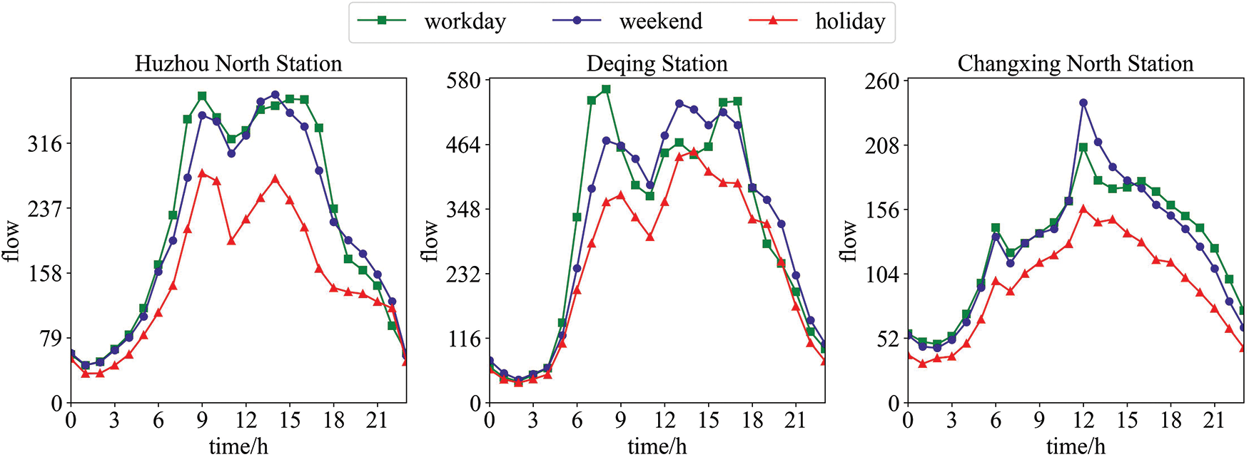
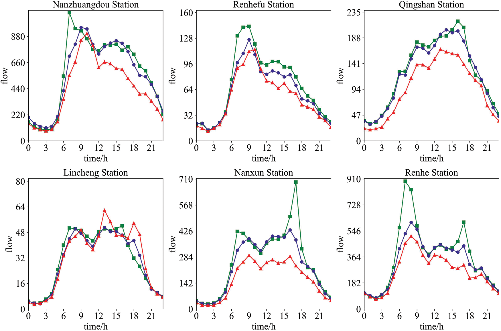
Figure 3: Excerpts from the 24-h average time series of different date types at 18 stations

Except for Lincheng Station, the holiday traffic of the other eight stations is lower than that of weekdays and weekends to a certain extent, which may be related to the fact that these areas are not popular tourist cities. The three traffic flows at each station are mainly concentrated in the time period from 6:00 to 18:00, and then begin to gradually decrease. Except Renhefu Station, there are two peak periods in the eight stations when the traffic is mainly concentrated, one peak between 6:00 and 9:00, and the other peak between 12:00 and 18:00. Overall, there is a trend of first growth and then decline, and then growth in decline. In general, Renhefu station has a peak period between 6:00 and 18:00, after which it begins to decline.

4.3.2 Analysis on Weather

To explore the influence of weather on traffic flow, we plot the 24-h average traffic flows under different weather conditions, nine of which are shown in Fig. 4. The 272-day real etc data of highways include sunny days, heavy rains, hazes, snowy days, and typhoons. Concretely, there were 179 sunny days and 93 days of heavy rain, haze, snow, typhoon, etc. Among the 93 days of special weather, the number of days with haze, snow, or typhoon is less than 10 days, so rainy days, haze, snow, and typhoon are collectively classified as other weather. Fig. 4 depicts 24-h traffic flow at different stations in sunny and other weather. It can be seen that the traffic flow on sunny days is not significantly different from that on other weather days, so weather factors have little influence on the traffic flow.

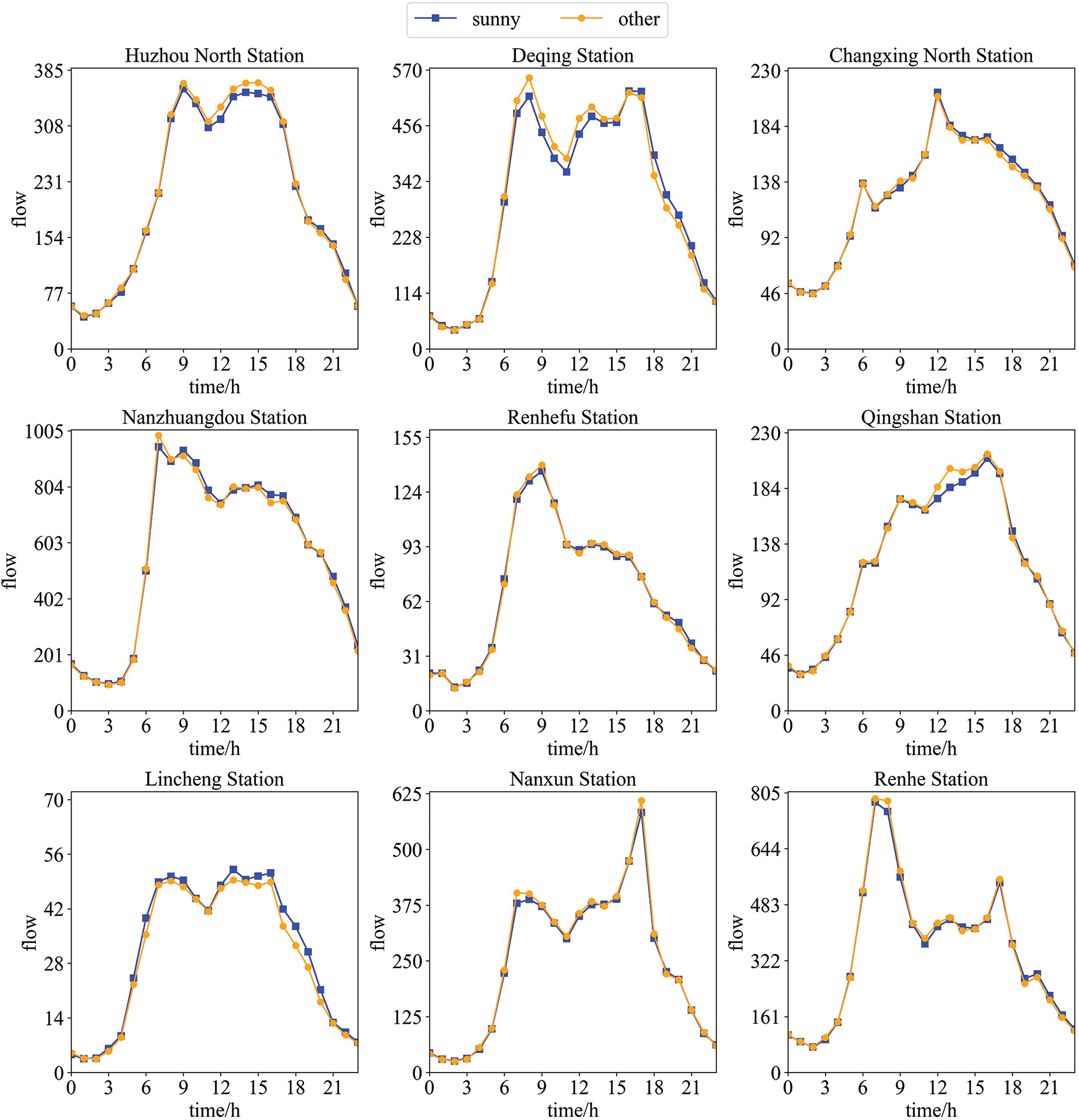
Figure 4: Excepts from 24-h average time series of different weather at 18 stations

4.3.3 Ablation Experiments

To verify the effectiveness of the proposed CALTM, we constructed ablation experiments on both holiday and weekend datasets. Fig. 5 presents the results of an ablation study on the model’s S2M2 module, represented by MSE figure. Comparative experiments were conducted to investigate the impact of incorporating retrieved similar sequences into the model. Four advanced observation days (Tahead=1, Tahead=3, Tahead=5, and Tahead=7) were considered for both the holiday datasets (H3 and H7) and weekend datasets (W3 and W7). The experimental results demonstrate that the CALTM model with the S2M2 module consistently achieved significantly lower MSE value than the model without this retrieval mechanism, particularly on the holiday datasets. The most substantial improvement was observed when using Tahead=5, where the MSE value decreased by 78.67%. On the weekend dataset, the most significant improvement was observed at Tahead=7, with a reduction in MSE value of 43.46%. These findings indicate that similarity sequence retrieval effectively enhances feature extraction and improves the model’s overall performance.

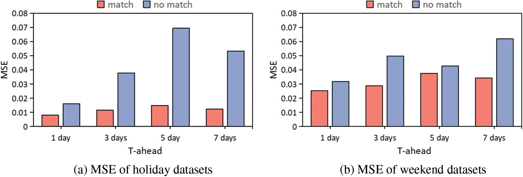
Figure 5: Ablation experiments on holidays and weekends

Fig. 6 showcases the traffic forecast results of the CALTM model and other comparative models across four datasets (H7, H3, W7, and W3) for two toll stations. Each dataset corresponds to specific conditions, denoted by the number of days ahead (e.g., H7 represents the holiday dataset with Tahead=7). Notably, the CALTM model demonstrates the most prominent forecasting results at the Nanzhuang Dou station, exhibiting a highly accurate and well-fitting forecasting curve. The N-BEATS model also performs well, while the LSTM and the statistical-based SeasESOpt models exhibit poor performance, characterized by unstable forecasting curves. Similar patterns were observed across other toll stations as well. By observing the traffic flow on different datasets within the same tollbooth, we discovered that the holiday datasets generally outperformed the weekend datasets, particularly when considering similar datasets with smaller Tahead values. Additionally, when comparing different toll stations within the same dataset, we found that stations with higher traffic volumes exhibited better overall forecasting performance. Obviously, Nanzhuangdou station, with the higher traffic volume, consistently achieved the more accurate and fitting forecasting results than Huzhounanlushan station.

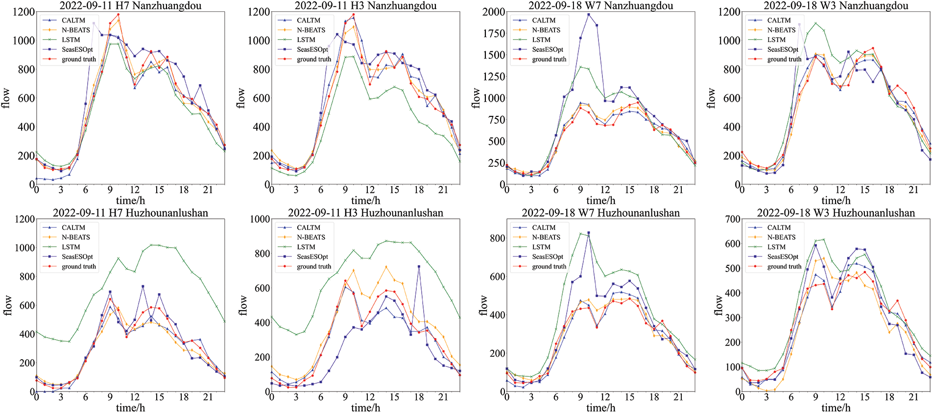
Figure 6: Visual analysis of forecasting results of different methods at two toll stations, including CALTM, N-BEATS, LSTM, SeasESOpt and groundtruth

5  Conclusion

In this paper, we propose a novel plug-in module, namely S2M2, that can be applied to all time series problems with rich contextual features to identify similar historical time series. Furthermore, We propose CALTM, a holiday traffic flow forecasting model framework that combines scene and sequential context to address the challenge of insufficient long-term sequence forecast capability in recurrent neural networks. We then evaluate the proposed model on a real-world etc dataset of G25–G50 expressway, which provides actual traffic measurement data for the Zhejiang sections of Changshen Expressway and Shanghai-Chongqing Expressway. The experimental results demonstrate that our proposed model substantially reduces the forecasting MSE compared with the mainstream methods. Additionally, we have collaborated with the local transportation design institute to deploy the CALTM model for practical application.

There are some ideas that we would have liked to add during the representation and the forecasting functions to improve the accuracy, such as the topology of traffic networks, time-series graph neural networks, and correlation of traffic flow. Moreover, if the scene is special and cannot extract enough similar scenes for forecasting, some few-shot learning approaches could be utilized to train a model on a small number of matched samples.

Acknowledgement: The authors would like to thank the support of advanced computing resources provided by the Supercomputing Center of Hangzhou City University.

Funding Statement: This research was funded by the Natural Science Foundation of Zhejiang Province of China under Grant (No. LY21F020003), Zhejiang Science and Technology Plan Project (No. 2021C02060), and the Scientific Research Foundation of Hangzhou City University (No. X-202206).

Author Contributions: The authors confirm contribution to the paper as follows: study conception and design: C. Jin, J. Chen, J. Ying; data collection: J. Chen, S. Wu; analysis and interpretation of results: J. Chen, S. Wu, H. Wu; draft manuscript preparation: C. Jin, J. Chen, S. Wu, H. Wu, S. Wang, J. Ying. All authors reviewed the results and approved the final version of the manuscript.

Availability of Data and Materials: The data obtained and/or analyzed during the current study are available from the corresponding author on reasonable request.

Conflicts of Interest: The authors declare that they have no conflicts of interest to report regarding the present study.

References

1. Williams, B. M., Hoel, L. A. (2003). Modeling and forecasting vehicular traffic flow as a seasonal Arima process: Theoretical basis and empirical results. Journal of Transportation Engineering, 129(6), 664–672. [Google Scholar]

2. Xu, D. W., Wang, Y. D., Jia, L. M., Qin, Y., Dong, H. H. (2017). Real-time road traffic state prediction based on Arima and Kalman filter. Frontiers of Information Technology & Electronic Engineering, 18(2), 287–302. [Google Scholar]

3. Tang, J., Chen, X., Hu, Z., Zong, F., Han, C. et al. (2019). Traffic flow prediction based on combination of support vector machine and data denoising schemes. Physica A: Statistical Mechanics and its Applications, 534, 120642. [Google Scholar]

4. Yang, L., Yang, Q., Li, Y., Feng, Y. (2019). K-nearest neighbor model based short-term traffic flow prediction method. 2019 18th International Symposium on Distributed Computing and Applications for Business Engineering and Science (DCABES), Wuhan, China, IEEE. [Google Scholar]

5. Huang, W., Song, G., Hong, H., Xie, K. (2014). Deep architecture for traffic flow prediction: Deep belief networks with multitask learning. IEEE Transactions on Intelligent Transportation Systems, 15(5), 2191–2201. [Google Scholar]

6. Tian, Y., Pan, L. (2015). Predicting short-term traffic flow by long short-term memory recurrent neural network. 2015 IEEE International Conference on Smart City/SocialCom/SustainCom (SmartCity), Chengdu, China, IEEE. [Google Scholar]

7. Fu, R., Zhang, Z., Li, L. (2016). Using LSTM and GRU neural network methods for traffic flow prediction. 2016 31st Youth Academic Annual Conference of Chinese Association of Automation (YAC), Wuhan, China, IEEE. [Google Scholar]

8. Kang, D., Lv, Y., Chen, Y. Y. (2017). Short-term traffic flow prediction with LSTM recurrent neural network. 2017 IEEE 20th International Conference on Intelligent Transportation Systems (ITSC), Yokohama, Japan, IEEE. [Google Scholar]

9. Zhao, W., Gao, Y., Ji, T., Wan, X., Ye, F. et al. (2019). Deep temporal convolutional networks for short-term traffic flow forecasting. IEEE Access, 7, 114496–114507. [Google Scholar]

10. Zhao, L., Song, Y., Deng, M., Li, H. (2017). Temporal graph convolutional network for urban traffic flow prediction method. arXiv preprint arXiv:1811.05320. [Google Scholar]

11. Zhao, L., Song, Y., Zhang, C., Liu, Y., Wang, P. et al. (2019). T-GCN: A temporal graph convolutional network for traffic prediction. IEEE Transactions on Intelligent Transportation Systems, 21(9), 3848–3858. [Google Scholar]

12. Hou, F., Zhang, Y., Fu, X., Jiao, L., Zheng, W. (2021). The prediction of multistep traffic flow based on AST-GCN-LSTM. Journal of Advanced Transportation, 2021, 1–10. [Google Scholar]

13. Han, X., Gong, S. (2022). LST-GCN: Long short-term memory embedded graph convolution network for traffic flow forecasting. Electronics, 11(14), 2230. [Google Scholar]

14. Wang, Y., Jing, C., Xu, S., Guo, T. (2022). Attention based spatiotemporal graph attention networks for traffic flow forecasting. Information Sciences, 607, 869–883. [Google Scholar]

15. Zhu, J., Han, X., Deng, H., Tao, C., Zhao, L. et al. (2022). KST-GCN: A knowledge-driven spatial-temporal graph convolutional network for traffic forecasting. IEEE Transactions on Intelligent Transportation Systems, 23(9), 15055–15065. [Google Scholar]

16. Jin, C., Ruan, T., Wu, D., Xu, L., Dong, T. et al. (2021). HetGAT: A heterogeneous graph attention network for freeway traffic speed prediction. Journal of Ambient Intelligence and Humanized Computing, 1–12. https://link.springer.com/article/10.1007/s12652-020-02807-0 (accessed on 25/11/2023) [Google Scholar]

17. Li, Y., Chai, S., Ma, Z., Wang, G. (2021). A hybrid deep learning framework for long-term traffic flow prediction. IEEE Access, 9, 11264–11271. [Google Scholar]

18. Olivares, K. G., Challu, C., Marcjasz, G., Weron, R., Dubrawski, A. (2023). Neural basis expansion analysis with exogenous variables: Forecasting electricity prices with NBEATSx. International Journal of Forecasting, 39(2), 884–900. [Google Scholar]

19. Yue, Z., Wang, Y., Duan, J., Yang, T., Huang, C. et al. (2022). TS2Vec: Towards universal representation of time series. Proceedings of the AAAI Conference on Artificial Intelligence, vol. 36. BC, Canada. [Google Scholar]

20. Chen, Z., Wu, B., Li, B., Ruan, H. (2021). Expressway exit traffic flow prediction for etc and mtc charging system based on entry traffic flows and LSTM model. IEEE Access, 9, 54613–54624. [Google Scholar]

21. Hossain, M. N., Ahmed, N., Ullah, S. W. (2022). Traffic flow forecasting in intelligent transportation systems prediction using machine learning. 2022 International Conference on Futuristic Technologies (INCOFT), Belgaum, India, IEEE. [Google Scholar]

22. Zhang, L., Liu, W., Feng, L. (2021). Short-term traffic flow prediction based on improved neural network with GA. 2021 IEEE International Conference on Artificial Intelligence and Computer Applications (ICAICA), Dalian, China, IEEE. [Google Scholar]

23. Holt, C. C. (2004). Forecasting seasonals and trends by exponentially weighted moving averages. International Journal of Forecasting, 20(1), 5–10. [Google Scholar]

24. Winters, P. R. (1960). Forecasting sales by exponentially weighted moving averages. Management Science, 6(3), 324–342. [Google Scholar]

25. Hyndman, R. J., Athanasopoulos, G. (2018). Forecasting: Principles and practice. OTexts. https://otexts.com/fpp3/ (accessed on 25/11/2023) [Google Scholar]

26. Hyndman, R. J., Khandakar, Y. (2008). Automatic time series forecasting: The forecast package for R. Journal of Statistical Software, 27, 1–22. [Google Scholar]

27. Atluri, S. N., Zhu, T. (1998). A new Meshless Local Petrov-Galerkin (MLPG) approach in computational mechanics. Computational Mechanics, 22(2), 117–127. [Google Scholar]

28. Cho, K., van Merriënboer, B., Gulcehre, C., Bahdanau, D., Bougares, F. et al. (2014). Learning phrase representations using RNN encoder-decoder for statistical machine translation. arXiv preprint arXiv:1406.1078. [Google Scholar]

29. Bai, S., Kolter, J. Z., Koltun, V. (2018). An empirical evaluation of generic convolutional and recurrent networks for sequence modeling. arXiv preprint arXiv:1803.01271. [Google Scholar]