Distributed Stochastic Optimization with Compression for Non-Strongly Convex Objectives

1  Introduction

In modern machine learning problems, datasets are frequently too large to be processed by a single machine or may be distributed across multiple computing nodes due to legal restrictions or cost considerations. In such scenarios, distributed learning has emerged as a viable solution to train models in a decentralized fashion. Each computing node trains on its local data samples, and communicates with other nodes to exchange information and update model parameters. This approach can significantly reduce processing time and has gained increasing attention in recent years.

Formally, we consider an optimization problem of the form

x∗=arg minx∈Rd⁡[f(x)=1n∑i=1nfi(x)],(1)

where fi:Rd→R is the local objective function of computing node (alternatively referred to as a worker) i for i∈{1,⋯,n}, x usually refers to the neural network model parameter, and each fi is determined by the local dataset of node i, i.e.,

fi(x)=1mi∑j=1miFi(x,ζj),(2)

where mi denotes the number of data samples of node i, ζj represents one data sample, and Fi:Rd×Ω→R is the loss function. For example, in a regression problem, a square loss function is commonly used as Fi(⋅).

Consensus-based gradient descent algorithms are extensively researched and employed in distributed learning owing to their simplicity and efficiency. These algorithms enable nodes to exchange parameters with neighboring nodes and incorporate new information from received messages to drive the parameters toward the global average parameter value. Meanwhile, each node computes gradients using its local data samples and updates its parameters using the gradient descent methods.

One limitation of these algorithms is the requirement for exact parameter transmission among nodes, which can be challenging in scenarios where there are restrictions on data transmission amount or high communication latency (e.g., with large neural networks [1] or limited network bandwidth). In such cases, compressing the parameters becomes necessary. However, parameter compression usually results in a decrease in the convergence rate. To address this challenge, Koloskova et al. proposed CHOCO-SGD [2], which was a compressed distributed algorithm designed for strongly convex objective functions. CHOCO-SGD allows for both biased and unbiased compression operators and can achieve arbitrary compression precision. Arbitrary compression precision means that any compression fidelity 0<ω≤1 (w=1 indicating no compression) can guarantee the same convergence rate order as the no-compression equivalent.

However, strong convexity is a restrictive assumption that may not hold in various practical applications, such as in operations research and machine learning. For instance, consider the Lasso problem [3] with an objective function represented as ∑i=1m12(⟨di,x⟩−li)2+β‖x‖1, where i∈{1,⋯,m} denotes the data index, β denotes the regularization coefficient, and di and li represent data features and labels, respectively. In this case, each component function is non-strongly convex, as well as the global objective. Another well-known example is logistic regression [4], where the objective is ∑i=1mlog(1+exp(−li⟨di,x⟩). Therefore, it is crucial to investigate the behavior and performance of CHOCO-SGD for objectives that are non-strongly convex in nature. The main contributions are summarized as follows:

•   We establish a compression fidelity bound for CHOCO-SGD, ensuring its convergence over non-strongly convex functions. This criterion serves as a valuable guideline for researchers and engineers when applying CHOCO-SGD in practical scenarios.

•   We rigorously prove that within the compression fidelity threshold, CHOCO-SGD achieves the same convergence rate order as DSGD over non-strongly convex objectives, and compression fidelity only affects the higher-order terms in the rate. This means that CHOCO-SGD effectively reduces the transmitted data without compromising training efficiency.

•   We conduct comprehensive experiments to validate our theoretical results. The numerical outcomes show that when controlling compression fidelity above the lower bound, CHOCO-SGD effectively reduces communication costs, while remains a comparable convergence rate to that of DSGD. Additionally, our experiments reveal that CHOCO-SGD fails to converge when the fidelity falls below acceptable limits, implying that this algorithm cannot achieve arbitrary compression fidelity on non-strongly convex objectives. Moreover, we also observe that CHOCO-SGD cannot converge in time-varying network topologies.

Notations. In this paper, we use uppercase letters like X, A to denote various matrices, including parameter matrix, gradient matrix, weight matrix, etc. Lowercase letters with subscripts are used to denote vectors, for example, xi means the parameter vector of node i. In terms of some special matrices and vectors, we use 1 for a column vector whose elements are all 1 and I for the identity matrix whose size can be inferred from the context. We uniformly use ‖⋅‖ without subscripts for norm notations. When the norm is on a vector, it should represent the ℓ2 norm, but when it is on a matrix, it should be the Frobenius norm.

2  Related Work

Consensus algorithm. For the distributed optimization problem, we want every node to reach an agreement on the global parameter value. The agreement means finding the average of n initial values stored on n nodes [5,6]. So, the consensus problem can be regarded as a subproblem of distributed optimization problem. There are a plethora of research works conducted to explore the consensus problem. It has been proved that the consensus problem can be addressed in the sense of linear convergence on undirected graph [6].

Distributed optimization. On the basis of consensus algorithms, researchers proposed many distributed gradient-based algorithms [7–12]. In undirected topology, Nedic et al. [7] and Yuan et al. [8] analyzed the convergence of Decentralized Stochastic Gradient Descent algorithm (DSGD) on non-strongly convex objective functions. Lian et al. proved that for nonconvex and Lipschitz-smooth objective functions, DSGD can converge to a stationary point with the rate O(1nT) [13], where T denotes the number of episodes. Furthermore, Shi et al. proposed the EXTRA algorithm that had linear convergence rate for strongly convex objectives [14]. Assran et al. further addressed challenges introduced by directed graphs by designing the SGP algorithm based on DSGD [15]. More related algorithms has been reviewed in [16,17].

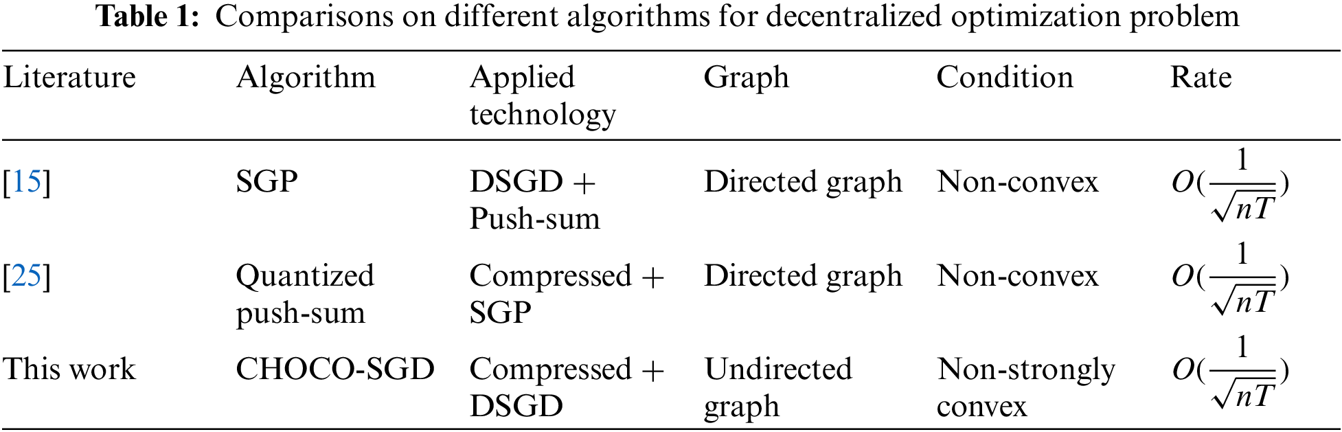
Parameter/gradient compression. With the rapid growth of learning models, traditional distributed learning faces significant communication pressure. As a result, Researchers have increasingly focused on designing communication-efficient algorithms [2,18–24]. The proposed methods can generally be classified into three main categories. The first category is quantization. Instead of transmitting precise vectors (such as model parameters or gradients), nodes exchange limited bits that approximate the original vectors. The second category is sparsification, where only a few elements of a vector are transmitted accurately, while the remaining elements are forced to be zero. The third category involves transmitting parameters in some iterations rather than in every iteration. This aims to reduce the amount of transmitted information. All these methods aim to find the optimal parameter value by transmitting less information. Therefore, in this paper, we use the term compression to encompass these methods. Kolovaskova et al. proposed the CHOCO-SGD algorithm [2], a distributed stochastic algorithm over undirected graphs. This algorithm allows for arbitrary compression precision and has been proven to converge for strongly convex objectives. Taheri et al. [25] extended this algorithm to directed graphs for both convex and nonconvex objectives based on the SGP algorithm [15]. Different from this work, our study is based on undirected graphs. Table 1 further illustrates the highlights of this work and the differences between the work involved.

3  CHOCO-SGD Algorithm

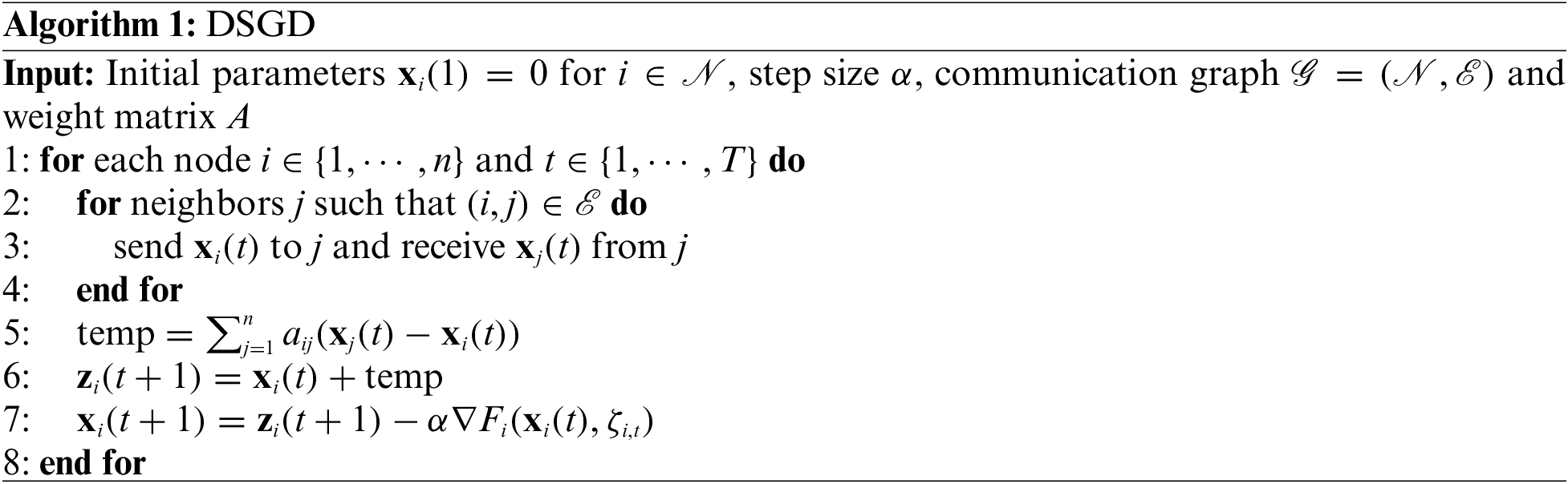
In this section, we will introduce the basic knowledge of distributed optimization and present the classic Distributed Stochastic Gradient Descent (DSGD) algorithm. Additionally, we will discuss the fundamental ideas underlying the CHOCO-SGD algorithm.

We assume that the computing nodes are distributed across an undirected graph 𝒢=(𝒱,ℰ), where 𝒱 and ℰ represent the set of nodes and edges, respectively. The DSGD algorithm is an efficient method to solve the distributed optimization problem in Eq. (1). It consists of two key components: consensus, also referred to as gossip, and parameter updates. The consensus step aims to achieve parameter agreement among all nodes. Specifically, we denote the local parameter of node i as xi, and perform the following parameter aggregation process:

xi(t+1)=∑j=1naijxj(t),(3)

where t denotes the iteration number and aij denotes the weight assigned by node i to node j. For compatibility with the underlying graph structure, aij is set to be positive if and only if edge(i,j)∈ℰ or i=j. This ensures that only neighboring nodes, as determined by the graph, can communicate and exchange their parameters. By using a matrix A=(aij)n×n 1 to incorporate all the weights, it has been proven that when A is row stochastic (i.e., each row of A sums to one and all the entries are non-negative), the parameters of all nodes can reach a consensus. This implies that each parameter xi(t) will converge to the average of the initial values 1n∑i=1nxi(1) [26]. This consensus algorithm enables the nodes to synchronize their parameter values.

The second component of the DSGD algorithm involves parameter updates using stochastic gradient descent. Combining these components, the update rule of DSGD is given as follows:

xi(t+1)=∑j=1naijxj(t)−α∇Fi(xi(t),ζi,t),(4)

where ∇Fi(xi(t),ζi,t) represents the gradient of the local objective function evaluated at xi(t) using the data batch ζi,t, and α denotes the learning rate. This update rule combines the consensus step, which ensures parameter agreement, with the gradient descent step, which drives the parameters towards optimal values. We formally present the DSGD algorithm in Algorithm 1. Under some constraints, extensive studies [16] have demonstrated that the DSGD algorithm achieves a convergence rate of O(1nT) on non-strongly convex objective functions, where T denotes the number of episodes.

However, when dealing with massive training models, the DSGD algorithm encounters a communication bottleneck. To address this limitation, a straightforward yet effective solution is to compress the parameters before transmitting them over the network. For this purpose, We introduce a compression operator denoted as Q, along with the definition of compression fidelity ω, which indicates the ratio of preserved information. A higher value of ω signifies a greater fidelity, implying that less information is discarded during the compression process. The value of ω satisfies the following assumption.

Assumption 3.1. The compression operator Q satisfies

EQ‖Q(x)−x‖2≤(1−ω)‖x‖2.

We take the expectation in this context because there might be inherent randomness in the compression operators, such as in the case of randomized gossip discussed later. It is worth noting that when ω=1, the compressed parameter Q(x) should ideally be the same as x (almost surely, although we may disregard negligible difference). And we state that the operator Q can be either biased or unbiased, encompassing a wide range of compression techniques.

Example 3.1. Examples of compression

•   randomized gossip:

Q(x)={x,with probability p0,with probability 1−p,

where p∈(0,1]. We can find ω=p.

•   Top-k sparsification [20]: for a parameter vector x∈Rd, we select k dimensions with the highest magnitude, where k∈{1,2,⋯,d}. Subsequently, we transmit a compressed version of the parameter vector, retaining only the selected k items while setting all other positions to 0. It is worth noting that the compression fidelity in this case can be calculated as ω=kd.

Through conducting simple experiments, one can observe that when integrating compression directly into the transmitted parameter in Algorithm 1 (i.e., replacing the transmission of xi(t) with Q(xi(t))), the algorithm typically fails to converge. The primary reason behind this behavior stems from the magnitude of xi(t). In general, it lacks a bound, meaning its magnitude is not necessarily close to zero. As a result, the error introduced by compressing (such as forcing certain positions to be zero) becomes difficult to control. Hence, it is important to employ the compression operator appropriately and judiciously.

Based on Assumption 3.1, CHOCO-SGD was proposed and is presented in Algorithm 2. As the transmitted parameters are compressed and inexact, each node i needs to maintain n additional auxiliary variables {x^j(t),j∈𝒩} to approximate the true parameters of all n nodes. Specifically, for each node i∈𝒩, the newly added auxiliary variable x^j(t) represents an estimation of the actual local parameter of node j. In Algorithm 2, instead of sending the compressed parameters, the nodes transmit the compressed value of the difference between the true local parameter and its estimator. Subsequently, upon receiving messages from neighboring nodes, every node updates its estimators of parameters of other nodes, denoted as {x^1(t+1),⋯,x^n(t+1)}. If the estimations maintained by each node are accurate, the error introduced by compression is minimal and will eventually vanish. It has been proven that Q(x^i(t)−xi(t)) asymptotically equals to x^i(t)−xi(t), which does not hold for Q(xi(t)) and xi(t).

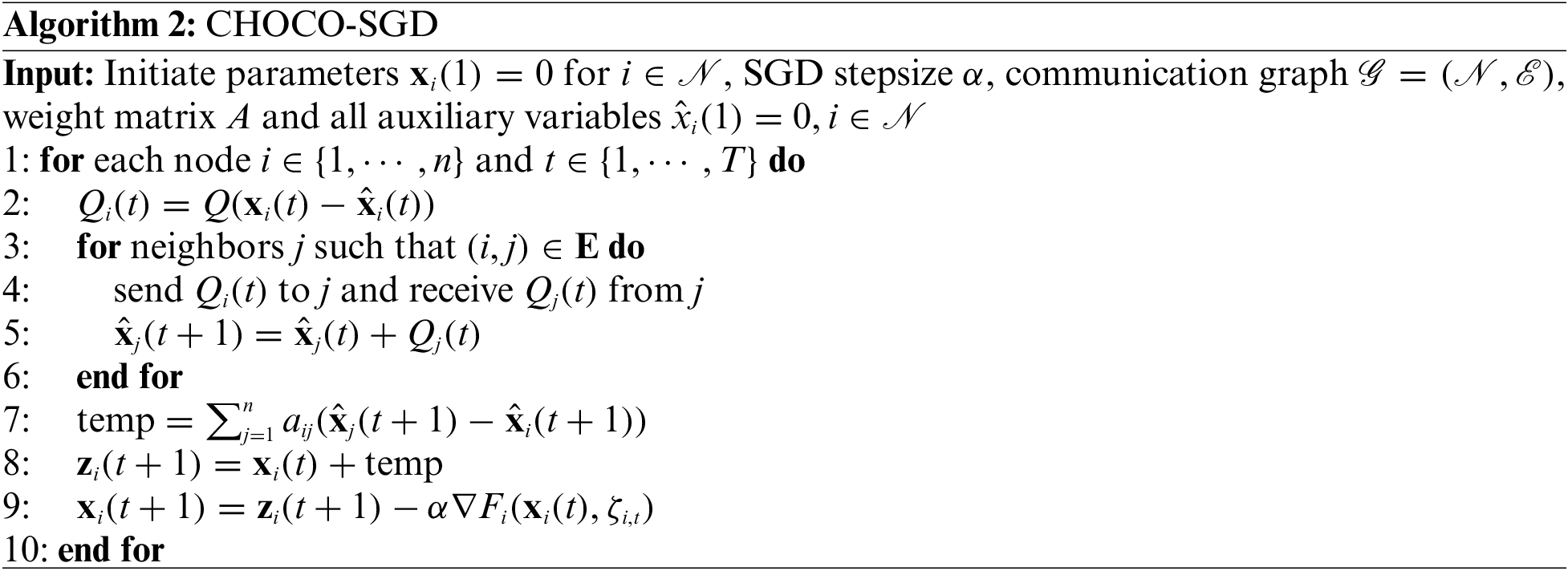
Koloskova et al. [2] has proved that Algorithm 2 achieved a convergence rate of O(1T) on strongly convex objective functions when specific parameters such as the step size and regularization parameter were appropriately chosen. Furthermore, it has been established that this algorithm can converge with arbitrary compression fidelity, indicating minimal communication pressure. To evaluate its potential in practical scenarios, we investigate its convergence properties on non-strongly convex objective functions.

4  Convergence Analysis for Non-Strongly Convex Objectives

In this section, we begin by introducing assumptions regarding the underlying graph structure. As mentioned previously, we use 𝒢=(𝒱,ℰ) to denote the undirected graph and use 𝒩i to denote all the neighbors of node i together with itself, i.e., 𝒩i={j:(i,j)∈ℰ}∪{i}. We have a couple of well-accepted assumptions in distributed optimization, which are related to the graph structure and the corresponding weight matrix.

Assumption 4.1. The underlying graph structure 𝒢 is connected.

Assumption 4.2. Given the aggregation weights aij, the weight matrix A=(aij)n×n is doubly stochastic and non-negative, i.e.,

A⋅1=1,AT1=1,aij≥0,

where A satisfies σ2<1, where σ2 denotes the second largest singular value of A.

Remark 4.1. Under the undirected graph setting, a doubly stochastic matrix can be easily found. Given an undirected graph 𝒢, with its adjacent matrix A0, the degree matrix D and the maximum degree Δ, it can be directly shown that A0+(Δ+1)I−DΔ+1 is a valid doubly stochastic matrix [27].

We next introduce several basic assumptions on the objective function and its gradients. Note that these assumptions are common in first-order continuous optimization.

Assumption 4.3. Each local objective function fi(⋅) is convex, i.e.,

fi(y)≥fi(x)+⟨∇fi(x),y−x⟩,∀x,y∈Rd,

and L-smooth, i.e., there exists a constant L>0 (for all i∈𝒩), such that

fi(y)≤fi(x)+⟨∇fi(x),y−x⟩+L2‖y−x‖2,∀x,y∈Rd.

The definition of L-smooth is equivalent to the following inequality:

‖∇fi(x)−∇fi(y)‖≤L‖x−y‖,∀x,y∈Rd.

Assumption 4.4. There exists a constant M, such that

Eζi,t‖∇Fi(x)‖2≤M2,∀x∈Rd.

Assumption 4.5. There exists a constant σ, such that

Eζi,t‖∇Fi(x)−∇fi(x)‖2≤σ2,∀x∈Rd.

Assumptions 4.4 and 4.5 bound the local gradients and variance with respect to data samples, respectively. The latter assumption can be easily satisfied when the dataset across nodes is independent and identically distributed. Besides, the following asymptotic property of A implies that all the elements in At will be distributed in the vicinity of 1m as t→∞.

Lemma 4.1. If A∈Rn×n is a doubly stochastic matrix with σ2<1, then there exists constants λ∈(0,1) and C>0, such that

‖At−1n11T‖≤Cλt,

where At refers to the product of t matrices.

This lemma states that as matrix multiplication progresses, all elements of At converge to 1n. The detailed proof is presented in the appendix. With these assumptions and lemma, we can analyze the convergence properties of CHOCO-SGD for non-strongly convex objectives.

Theorem 4.1. Under Assumptions 3.1 and 4.1–4.5, and assume α≤18L, the CHOCO-SGD algorithm satisfies

1T∑t=1T(Ef(x¯(t))−f(x∗))≤E‖x∗‖2Tα+2σ2αn+24C2βLα2(1−λ)2+6C2M2Lα2(1−λ)2,(5)

where

ω>1−13+24n+384n2C2(1−λ)2,(6)

and x¯(t) denotes the average parameter after the t iterations, i.e., x¯(t)=X(t)1n. Notations C and λ come from Lemma 4.1, and

β=3(1−ω)nM2+96(1−ω)C2n2M2(1−λ)21−[(3+24n)(1−ω)+384n2(1−ω)C2(1−λ)2].(7)

Let α=O(nT), the right-hand side (RHS) of Eq. (5) will be equal to O(1nT)+O(nT). When T is large enough, the term nT is dominated by another term 1nT and the rate becomes O(1nT), which means that the convergence rate will be the same as DSGD (Algorithm 1) on non-strongly convex objectives, i.e., O(1nT). We can also discover that the compression fidelity ω and the graph spectral gap λ only appear in higher order terms O(nT) and have negligible influence on the convergence speed.

Furthermore, the expression ω>1−13+24n+384n2C2(1−λ)2 is a sufficient condition of achieving O(1nT) convergence rate. In this constraint, ω needs to be higher than a threshold related to the number of nodes and communication topology. We will demonstrate with experiments that CHOCO-SGD cannot converge on non-strongly convex objectives with low compression fidelity. In other words, the CHOCO-SGD algorithm does not allow arbitrary compression fidelity.

Proof. For simplicity, we let

X(t)=(x1(t),⋯,xn(t))X^(t)=(x^1(t),⋯,x^n(t))Z(t)=(z1(t),⋯,zn(t))∇(t)=(∇F1(x1(t),ζ1,t),⋯,∇Fn(xn(t),ζn,t))

and then the updating rule of Algorithm 2 can be expressed as

{Q(t)=Q(X(t)−X^(t))X^(t+1)=X^(t)+Q(t)Z(t+1)=X(t)+X^(t+1)(A−I)X(t+1)=Z(t+1)−α∇(t)(8)

Note that when we use the compression operator Q on a matrix, we mean compressing every column of that matrix. Since the underlying topology is fixed, node i and node j (i,j∈𝒩k) have the same estimator x^k for their common neighbor node k. Then we can use one matrix X^(t) to denote the original n×n auxiliary variables. Now, we start the proof by analyzing the distance between the average parameter in the (t+1)th iteration, denoted as x¯(t+1), and the optimum, denoted as x∗. By the updating rule and properties of A, we have

X(t+1)1=X(t)1+X^(t+1)(A−I)1−α∇(t)1=X(t)1−α∇(t)1.(9)

Dividing both sides by n and we can get x¯(t+1)=x¯(t)−α∇¯(t), where ∇¯(t) denotes the average gradient of ∇Fi(xi(t),ζi,t),i∈𝒩, i.e., ∇¯(t)=∇(t)1n. Then there exists

E‖x¯(t+1)−x∗‖2=E‖x¯(t)−x∗‖2+α2E‖∇¯(t)‖2−2αE⟨∇¯(t),x¯(t)−x∗⟩.(10)

The second term can be processed as follows:

E‖∇¯(t)‖2=E‖1n∑i=1n∇Fi(xi(t),ζi,t)‖2≤2E‖1n∑i=1n(∇Fi(xi(t),ζi,t)−∇fi(xi(t)))‖2+2E‖1n∑i=1n∇fi(xi(t))‖2,(11)

where the inequality comes from Cauchy-Schwarz inequality. The two terms in the right-hand side (RHS) of the last equation can be bounded as follows:

2E‖1n∑i=1n(∇Fi(xi(t),ζi,t)−∇fi(xi(t)))‖2=2n2∑i=1nE‖∇Fi(xi(t),ζi,t)−∇fi(xi(t)))‖2+2n2∑i≠i′E⟨∇Fi(xi(t),ζi,t)−∇fi(xi(t))), ∇Fi′(xi′(t),ζi′,t)−∇fi′(xi′(t)))⟩=2n2∑i=1nE‖∇Fi(xi(t),ζi,t)−∇fi(xi(t)))‖2+2n2∑i≠i′E⟨∇Fi(xi(t),ζi,t)−∇fi(xi(t))), Ei′∇Fi′(xi′(t),ζi′,t)−∇fi′(xi′(t)))⟩=2n2∑i=1nE‖∇Fi(xi(t),ζi,t)−∇fi(xi(t)))‖2≤2σ2n,(12)

where the last inequality applies Assumption 4.5. And for the second term, we have

2E‖1n∑i=1n∇fi(xi(t))‖2≤4n∑i=1nE‖∇fi(xi(t))−∇fi(x¯(t))‖2+4E‖1n∑i=1n∇fi(x¯(t))‖2≤4L2nE‖X(t)−x¯(t)1T‖2+8L(Ef(x¯(t))−f(x∗)),(13)

where the last inequality comes from Assumption 4.3 and the following result related to ‖∇fi(x¯(t))‖2:

f(x∗)≤f(x−1L∇f(x))≤f(x)+⟨∇f(x),−1L∇f(x)⟩+L2‖1L∇f(x)‖2=f(x)−12L‖∇f(x)‖2.(14)

Plugging the results in Eqs. (12) and (13) back into Eq. (11) yields the bound for E‖∇¯(t)‖2

E‖∇¯(t)‖2≤2σ2n+4L2nE‖X(t)−x¯(t)1T‖2+8L(Ef(x¯(t))−f(x∗)).(15)

Now we handle the third term in the RHS of Eq. (10) as follows:

E⟨∇¯(t),x¯(t)−x∗⟩=1n∑i=1nE[⟨∇fi(xi(t)),x¯(t)−xi(t)⟩+⟨∇fi(xi(t)),xi(t)−x∗⟩]≥E[f(x¯(t))−f(x∗)]−L2nE‖X(t)−x¯(t)1T‖2.(16)

In the first equation, we use Eζi,t∇Fi(xi(t),ζi,t)=∇fi(xi(t)) for i∈𝒩. The inequality comes from Assumption 4.3. Now, by substituting Eqs. (15) and (16) into Eq. (10), we obtain

E‖x¯(t+1)−x∗‖2≤E‖x¯(t)−x∗‖2−(2α−8Lα2)[Ef(x¯(t))−f(x∗)]+αL+4α2L2nE‖X(t)−x¯(t)1T‖2+2σ2α2n.(17)

Arranging this inequality and choosing α≤18L, so that 2−8Lα≥1, there exists

α[Ef(x¯(t))−f(x∗)]≤E‖x¯(t)−x∗‖2−E‖x¯(t+1)−x∗‖2+2σ2α2n+3αL2nE‖X(t)−x¯(t)1T‖2.(18)

By summing both sides for t from 1 to T, and dividing both sides by Tα, we can find that

1T∑t=1T(Ef(x¯(t))−f(x∗))≤E‖x∗‖2Tα+3L2nT∑t=1TE‖X(t)−x¯(t)1T‖2+2σ2αn,(19)

where we apply x¯(1)=0. Next we process E‖X(t)−x¯(t)1T‖2. Applying updating rules (8) and the recursion technique, we have

X(t)=X(t−1)A+[X^(t)−X(t−1)](A−I)−α∇(t−1)={X(t−2)A+[X^(t−1)−X(t−2)](A−I)−α∇(t−2)}A+[X^(t)−X(t−1)](A−I)−α∇(t−1)=X(1)At−1+∑k=0t−2[X^(t−k)−X(t−1−k)](A−I)Ak−α∑k=0t−2∇(t−1−k)Ak.(20)

Since A is doubly stochastic, we get

x¯(t)1T=X(t)11Tn=X(1)11Tn−α∑k=0t−2∇(t−1−k)11Tn.(21)

Therefore, after t iterations, the difference between the current parameter and the global average can be expressed as

E‖X(t)−x¯(t)1T‖2=E‖∑k=0t−2[X^(t−k)−X(t−1−k)](A−I)Ak−α∑k=0t−2∇(t−1−k)(Ak−11Tn)‖2≤2E‖∑k=0t−2[X^(t−k)−X(t−1−k)](A−I)Ak‖2+2α2E‖∑k=0t−2∇(t−1−k)(Ak−11Tn)‖2(22)

where we use X(1)=0 in the equality. With Lemma 4.1 and ‖A−I‖≤‖A‖+‖I‖≤2n, we can bound these two terms as follows:

2E‖∑k=0t−2[X^(t−k)−X(t−1−k)](A−I)Ak‖2=2E‖∑k=0t−2[X^(t−k)−X(t−1−k)](A−I)(Ak−11Tn)‖2≤2E(∑k=0t−2‖[X^(t−k)−X(t−1−k)](A−I)(Ak−11Tn)‖)2≤8nC2E(∑k=0t−2λk‖X^(t−k)−X(t−1−k)‖)2,(23)

and

2α2E‖∑k=0t−2∇(t−1−k)(Ak−11Tn)‖2≤2α2E(∑k=0t−2‖∇(t−1−k)(Ak−11Tn)‖)2≤2α2C2E(∑k=0t−2λk‖∇(t−1−k)‖)2(24)

Now, substituting Eqs. (23) and (24) to Eq. (22), we have

E‖X(t)−x¯(1)1T‖2≤8nC2E(∑k=0t−2λk‖X^(t−k)−X(t−1−k)‖)2+2α2C2E(∑k=0t−2λk‖∇(t−1−k)‖)2.(25)

We process the first term of RHS of Eq. (25) in the following way:

(∑k=0t−2λk‖X^(t−k)−X(t−1−k)‖)2=∑k=0t−2λ2k‖X^(t−k)−X(t−1−k)‖2+∑k≠k′λkλk′‖X^(t−k)−X(t−1−k)‖⋅‖X^(t−k′)−X(t−1−k′)‖≤∑k=0t−2λ2k‖X^(t−k)−X(t−1−k)‖2+12∑k≠k′λkλk′‖X^(t−k)−X(t−1−k)‖2+12∑k≠k′λkλk′‖X^(t−k′)−X(t−1−k′)‖2≤∑k=0t−2(λ2k+λk1−λ)‖X^(t−k)−X(t−1−k)‖2≤∑k=0t−22λk1−λ‖X^(t−k)−X(t−1−k)‖2,(26)

where the last inequality comes from λk≤11−λ. Applying the same technique to the second term of Eq. (25), we can get

E(∑k=0t−2λkE‖∇(t−1−k)‖)2≤∑k=0t−22λk1−λE‖∇(t−1−k)‖2≤2nM2(1−λ)2,(27)

where the last inequality applies Assumption 4.5. Then Eq. (25) can be written as

E‖X(t)−x¯(t)1T‖2≤16nC2∑k=0t−2λk1−λE‖X^(t−k)−X(t−1−k)‖2+4C2α2nM2(1−λ)2.(28)

This motivates us to bound ‖X^(t+2)−X(t+1)‖2 as follows:

E‖X^(t+2)−X(t+1)‖2=E‖X^(t+1)+Q(t+1)−X(t+1)‖2=E‖Q(X(t+1)−X^(t+1))−(X(t+1)−X^(t+1))‖2≤(1−ω)E‖X(t+1)−X^(t+1)‖2≤3(1−ω)(E‖X(t)−X^(t+1)‖2+α2E‖∇(t)‖2+E‖X^(t+1)(A−I)‖2)≤3(1−ω)E‖X(t)−X^(t+1)‖2+3(1−ω)α2nM2+6(1−ω)E‖(X^(t+1)−X(t))(A−I)‖2+6(1−ω)E‖(X(t)−x¯(t)1T)(A−I)‖2≤(3+24n)(1−ω)E‖X(t)−X^(t+1)‖2+3(1−ω)α2nM2+24n(1−ω)E‖X(t)−x¯(t)1T‖2,(29)

where the second and the last inequalities come from Eq. (8) and ‖A−I‖≤2n, respectively. For simplicity, we use L(t) to denote E‖X^(t+1)−X(t)‖2 and use K(t) to denote E‖X(t)−x¯(t)1T‖2. Then Eqs. (28) and (29) can be presented as

L(t+1)≤(3+24n)(1−ω)L(t)+3(1−ω)α2nM2+24n(1−ω)K(t),K(t)≤16nC2∑k=0t−2λk1−λL(t−1−k)+4C2α2nM2(1−λ)2.(30)

Next we use induction to prove that when ω>1−13+24n+384n2C2(1−λ)2, we have L(t)<βα2, for some β>0.

When t=1, we have L(1)=E‖X^(2)−X(1)‖2=0. Now we assume that the proposition is true for any index less than or equal to t. Then there exists

L(t+1)<(3+24n)(1−ω)βα2+3(1−ω)α2nM2+96(1−ω)C2n2M2(1−λ)2α2+384n2(1−ω)C2(1−λ)2βα2=[(3+24n)(1−ω)+384n2(1−ω)C2(1−λ)2]βα2+[3(1−ω)nM2+96(1−ω)C2n2M2(1−λ)2]α2.(31)

By setting ω>1−13+24n+384n2C2(1−λ)2 and choosing

β=3(1−ω)nM2+96(1−ω)C2n2M2(1−λ)21−[(3+24n)(1−ω)+384n2(1−ω)C2(1−λ)2],

the RHS of Eq. (31) will be less than βα2, and the proposition is proved.

With L(t)<βα2, we have

E‖X(t)−x¯(t)1T‖2=K(t)≤16nC2βα2(1−λ)2+4C2α2nM2(1−λ)2.(32)

By substituting this result to Eq. (19), we can get Theorem 4.1.

5  Experiments

5.1 Evaluation Setup

Testbed setting and topology. Our experiments are conducted on a testbed of 8 servers, each with an 8-core Intel Xeon W2140b CPU at 3.20 GHz, a 32 GB DDR4 RAM and a Mellanox Connect-X3 NIC supporting 10 GbE links. We use PyTorch as the experiment platform and employ its Distributed Data-Parallel Training (DDP) paradigm to realize parameter communication among the 8 servers. The main topology in experiments is a ring topology, as shown in Fig. 1a. Ring topology can be used in Local Area Network (LAN) or Wide Area Network (WAN) networks, and is also commonly used [28] in distributed learning.

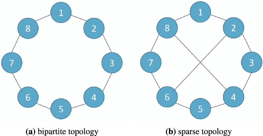
Figure 1: Undirected topologies with 8 nodes

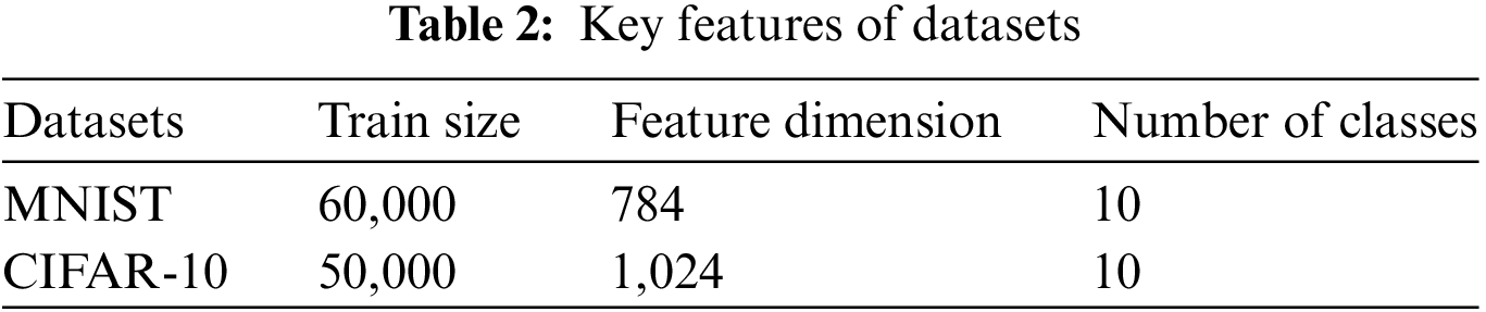
We consider a task where all nodes aim to classify images in the MNIST or CIFAR-10 dataset into 10 classes using a linear neural network. The key features of both datasets are listed in Table 2. The objective function for this task is cross-entropy loss. The cross-entropy loss of a data batch is defined as

1m∑i=1m∑j=1lp(xij)log(q(xij)),

where m and l represent the batch size and the number of categories, respectively. In this equation, q(xij) denotes the predicted probability of sample i belonging to class j, while p(xij) represents the true label, which is equal to 1 when sample i belongs to class j and 0 otherwise. The entire training dataset is divided into 8 equal partitions, each stored in an independent node. Unless otherwise specified, the learning rate and batch size are set to be 0.01 and 64, respectively.

5.2 Basic Results

We evaluate the performance of the CHOCO-SGD algorithm in comparison to the DSGD baseline. In CHOCO-SGD, we examine the efficacy of two compression operators outlined in Example 1: randomized gossip with p=0.7 and Top-k sparsification with ω=0.7. To align with our theoretical convergence criterion, the performance is evaluated based on the global loss computed on the global average parameter, denoted as f(x¯(t)). The model is trained for 25 episodes, where each episode corresponds to a pass through the entire dataset.

The results in Fig. 2a demonstrate that CHOCO-SGD and DSGD exhibit comparable convergence rates, with similar reductions in loss after the same number of episodes. To distinguish the curves, we scale the loss values to the range [0,1] with the following formula:

vscale=v−vminvmax−vmin,

where v is the real loss value in the training process, vmin and vmax denote the minimal and the maximal loss value achieved by three algorithms, respectively, and vscale represents the scaled loss value. The scaled results are depicted in Fig. 2b on a logarithmic scale. In the following context, the scaled training loss is processed likewise. In Fig. 2b, CHOCO-SGD and DSGD show only marginal differences in convergence rate. Furthermore, Figs. 2c and 2d (scaled) illustrate the comparison of the loss with respect to the number of transmitted bits. Remarkably, CHOCO-SGD, employing either randomized gossip or Top-k sparsification methods, achieves lower loss values while transmitting the same volume of data. This outcome can be attributed to the compression of certain values, which enables nodes to transmit fewer data in each communication round without adversely affecting the convergence rate. Similar results also appear on CIFAR-10 datasets, as shown in Fig. 3. CHOCO-SGD transmits about 1.2×1010 bits, while DSGD needs to transmit 1.7×1010 bits, when they achieve the same training error. These results align with our theoretical analysis, indicating that compression can effectively reduce the amount of transmitted data while exerting minimal influence on the convergence rate for non-strongly convex objectives, provided that the fidelity threshold is appropriately maintained.

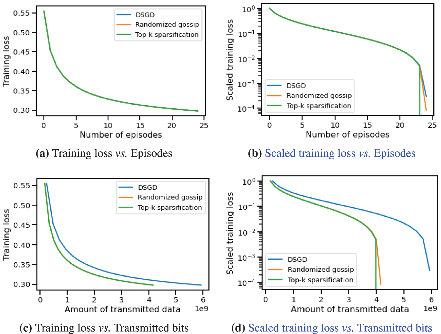
Figure 2: Training loss vs. episodes/transmitted data amount of CHOCO-SGD and DSGD on MNIST Dataset

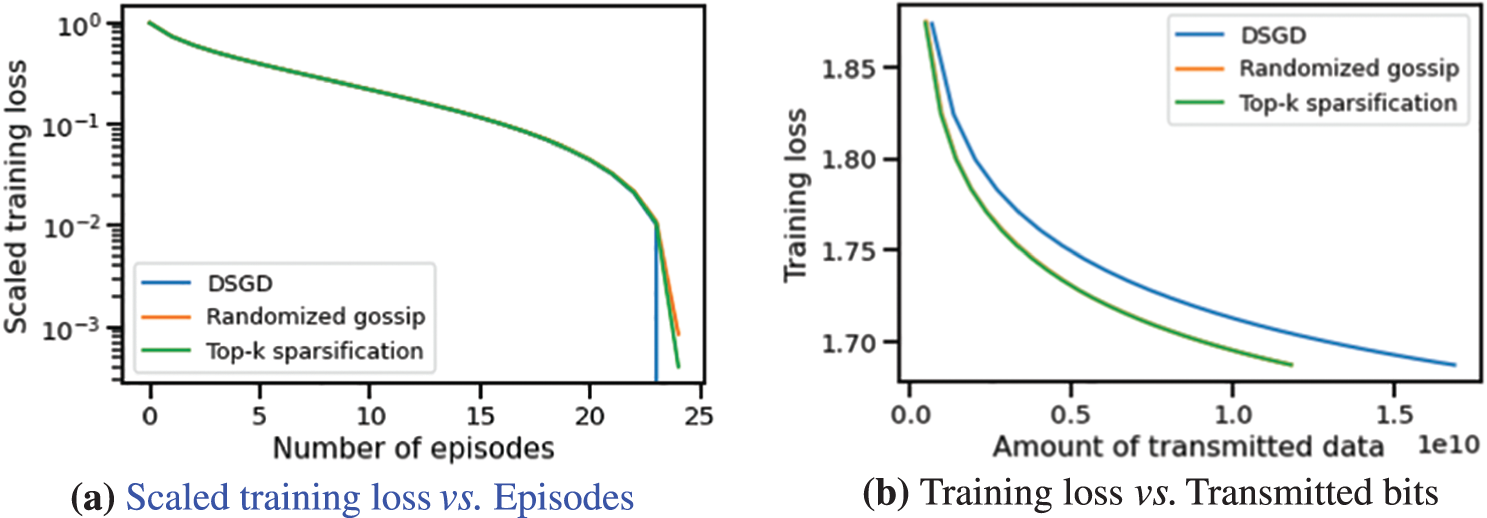
Figure 3: Training loss vs. episodes/transmitted data amount of CHOCO-SGD and DSGD on CIFAR-10 Dataset

5.3 Sensitivity to Compression Fidelity

To further investigate the impact of compression fidelity, we conduct several experiments by controlling the values of p and ω within the range of 0.9 to 0.5 for two compression operators. In randomized gossip, a smaller value of p increases the probability of transmitting full-zero parameters, which could lead to inaccuracies in x^j as described in Algorithm 2. The change in (scaled) training loss with respect to iterations and transmitted bits is depicted in Figs. 4a, 4b (MNIST) and Figs. 5a, 5b (CIFAR-10), respectively. We observe that lowering the value of p results in fewer transmission bits without slowing down the convergence rate. Similarly, the results obtained using Top-k sparsification, as shown in Figs. 4c, 4d and 5c, 5d indicate that reducing the number of bits, while maintaining ω within a certain threshold, ensures satisfactory convergence rates and reduces communication burden.

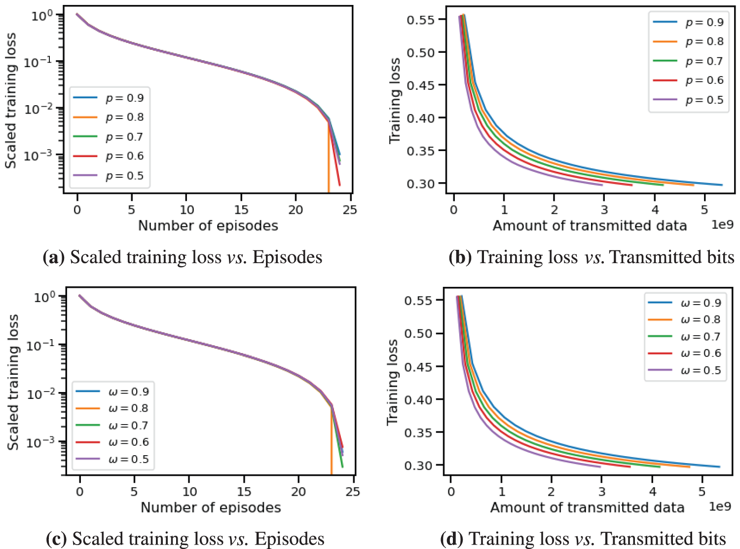
Figure 4: Training loss of CHOCO-SGD with randomized gossip (a), (b) and with Top-k sparsification (c), (d) on MNIST dataset. Both p and ω vary from 0.9 to 0.5

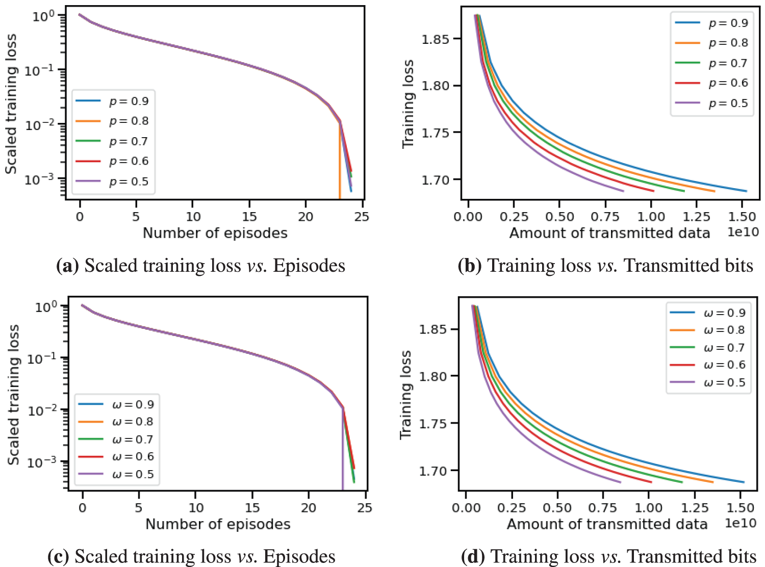
Figure 5: Training loss of CHOCO-SGD with randomized gossip (a), (b) and with Top-k sparsification (c), (d) on CIFAR-10 dataset. Both p and ω vary from 0.9 to 0.5

Furthermore, we conduct experiments to determine if CHOCO-SGD fails to converge when the compression fidelity is small for non-strongly convex objectives, as stated in Eq. (6). Specifically, for randomized gossip and Top-k sparsification, we set both p and ω to 0.4. Fig. 6 demonstrates that in an over-compression scenario, the training loss of CHOCO-SGD continues to increase, implying that the algorithm fails to converge. With these results, we empirically verify that within the context of non-strongly convex functions, CHOCO-SGD requires control of the compression fidelity within a threshold to ensure convergence, which differs from the situation with strongly convex functions. In other words, CHOCO-SGD cannot achieve arbitrary compression in a non-strongly convex scenario.

Figure 6: Convergence of CHOCO-SGD with low compression fidelity on MNIST dataset

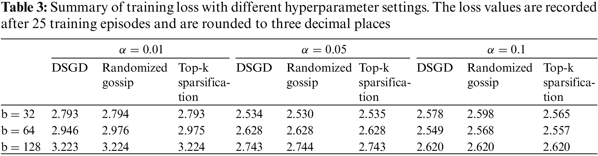
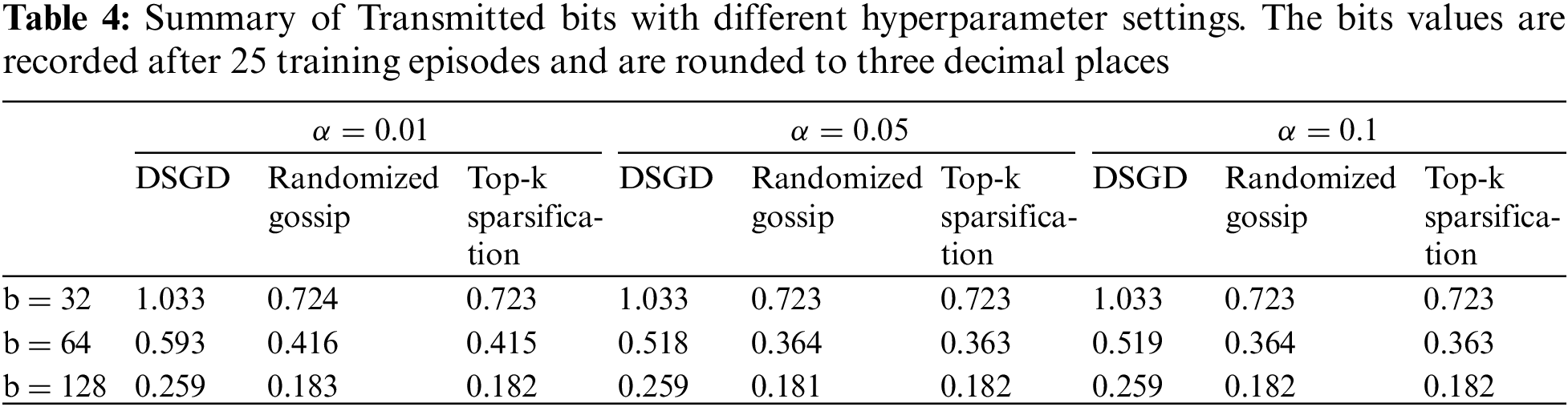
5.4 Robustness towards Learning Hyperparameters

In this section, we study the influence of hyperparameters (learning rate α and batch size b), on the convergence performance of the CHOCO-SGD algorithm for non-strongly convex functions. The compression fidelity is set to be p=ω=0.7. We test on three learning rates α=0.01,0.05,0.1 and three batch sizes b=32,64,128. The results are displayed in Tables 3 and 4. With the increase of the batch size, the final loss values of three algorithms after 25 training episodes become larger. Because each episode is one pass through the whole dataset, and larger batch size leads to fewer batches and thus fewer times of gradient descent and data transmission. Furthermore, the loss goes smaller when the learning rate gets larger, since the global parameter takes a larger step towards the global minimum. No matter in which hyperparameter setting, CHOCO-SGD and DSGD algorithms can achieve similar convergence error with the same training episodes, but CHOCO-SGD transmits less data amount. Furthermore, according to Table 4, the change of the learning rate has negligible influence on communication load, while larger batch size leads to fewer transmission data.

5.5 Applicability to Various Topologies

5.5.1 Investigating Different Fixed Topologies

To explore the algorithm’s applicability for non-strongly convex objectives, we test the convergence performance of CHOCO-SGD on two different topologies, as displayed in Fig. 7. Fig. 7a shows a bipartite topology, where nodes 1−4 and 5−8 are divided into two groups and each edge can only connect nodes in different groups. Besides, Fig. 7b displays a more sparse topology, where parameters can only be transmitted along one path in two directions. The compression fidelity is set to be p=ω=0.7 which is the same as basic experiments. Figs. 8 and 9 show the scaled training loss of MNIST dataset training on two topologies, respectively. In Fig. 8, CHOCO-SGD and DSGD have the same convergence speed, since they have similar loss values after the same training episodes. But the transmission amount of CHOCO-SGD, about 5×109, is much less than 7×109 of DSGD. Besides, in the sparser topology, Fig. 9b demonstrates that both algorithms can transmit fewer data to achieve convergence, but the transmitted amount of DSGD is 40% more than that of CHOCO-SGD. Therefore, these results further illustrate the robustness and applicability of CHOCO-SGD for non-strongly convex functions on various topologies.

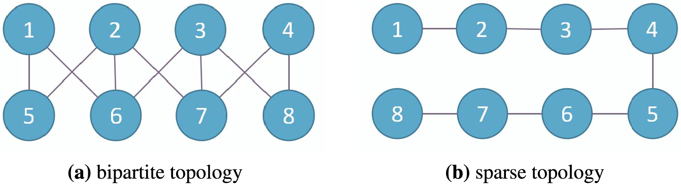
Figure 7: Different undirected and connected topologies

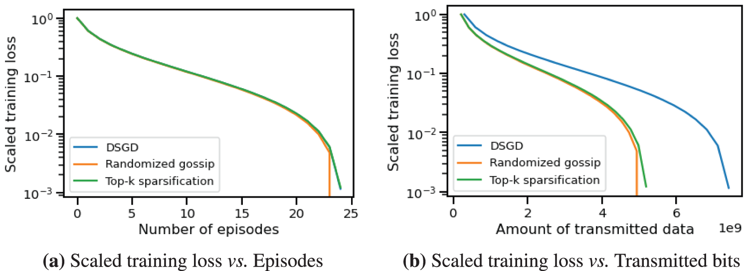
Figure 8: Training loss vs. episodes/transmitted data amount of CHOCO-SGD and DSGD on bipartite topology Fig. 7a

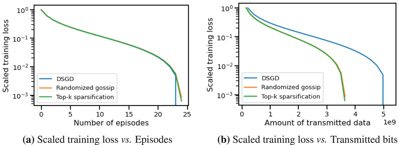
Figure 9: Training loss vs. episodes/transmitted data amount of CHOCO-SGD and DSGD on sparse topology Fig. 7b

5.5.2 Time-Varying Topologies

We further explore the impact of time-varying topologies on the convergence of CHOCO-SGD. The training topology alternates between the two graphs in Fig. 1. For instance, if the nodes are initially distributed over the left topology, in the next iteration, they will be connected according to the right topology. It is important to note that this setup still ensures connectivity (as stated in Assumption 4.1). We set the compression coefficients to p=ω=0.9 to reduce their influence on the convergence. Fig. 10 illustrates that CHOCO-SGD is not able to converge in a non-strongly convex and time-varying environment. Because some nodes receive parameters from specific neighbors inconsistently, resulting in an uncorrectable bias from true parameters and the algorithm diverges eventually.

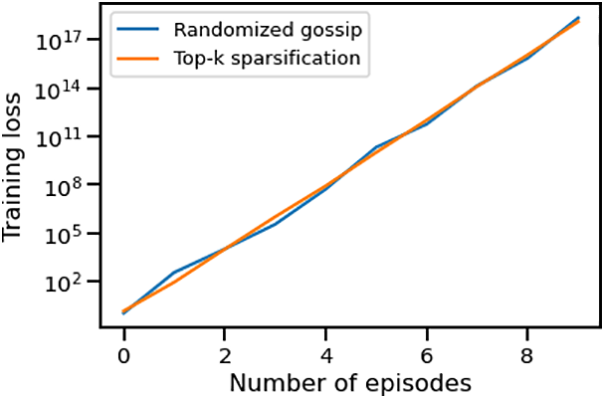
Figure 10: Convergence of CHOCO-SGD on time-varying topologies

6  Conclusion and Future Work

In this work, we study CHOCO-SGD algorithm in the case that the objective function is non-strongly convex. We provide the first theoretical analysis of this situation and prove that when controlling compression fidelity within a certain threshold, it has the same convergence rate order as DSGD. Experimental results validate the theoretical analysis by demonstrating that CHOCO-SGD converges more quickly than DSGD when transmitting the same data amount. Besides, a low compression fidelity and time-varying topology can make CHOCO-SGD not converge in the end.

There are several open topics worthy of investigating in our future work. The first one is to explore CHOCO-SGD’s performance in more complex non-convex scenarios, which can provide a deeper understanding of its capabilities. Besides, it will be meaningful to improve this algorithm to achieve arbitrary compression fidelity for non-strongly convex functions, since most real-world problems are non-strongly convex and such improvement can enhance CHOCO-SGD’s durability and applicability.

Acknowledgement: The authors are grateful for the theoretical support by Simiao Jiao. Besides, this paper’s logical rigor, integrity, and content quality have been greatly enhanced, so the authors also wish to express their appreciation to anonymous reviewers and journal editors for assistance.

Funding Statement: This work was supported in part by the Shanghai Natural Science Foundation under the Grant 22ZR1407000.

Author Contributions: The authors’ contributions to this manuscript are as follows: study conception: X.L., Y.X.; experiment design and data collection: X.L.; theoretical analysis, interpretation of results, and draft manuscript preparation: X.L., Y.X. All authors reviewed the results and approved the final version of the manuscript.

Availability of Data and Materials: The data, including MNIST and CIFAR-10 datasets, used in this manuscript is accessible via the following link: https://www.kaggle.com/datasets.

Conflicts of Interest: The authors declare that they have no conflicts of interest to report regarding the present study.

1a_ij represents the entry in the i^th row and the j^th column of A.

References

1. Jiang, X., Hu, Z., Wang, S., Zhang, Y. (2023). A survey on artificial intelligence in posture recognition. Computer Modeling in Engineering & Sciences, 137(1), 35–82. https://doi.org/10.32604/cmes.2023.027676 [Google Scholar] [PubMed] [CrossRef]

2. Koloskova, A., Stich, S., Jaggi, M. (2019). Decentralized stochastic optimization and gossip algorithms with compressed communication. International Conference on Machine Learning, Long Beach, California, USA. [Google Scholar]

3. Allen-Zhu, Z., Yuan, Y. (2016). Improved SVRG for non-strongly-convex or sum-of-non-convex objectives. International Conference on Machine Learning, New York, NY, USA. [Google Scholar]

4. Rajalakshmi, M., Rengaraj, R., Bharadwaj, M., Kumar, A., Naren Raju, N. et al. (2018). An ensemble based hand vein pattern authentication system. Computer Modeling in Engineering & Sciences, 114(2), 209–220. https://doi.org/10.3970/cmes.2018.114.209 [Google Scholar] [CrossRef]

5. Saber, R. O., Murray, R. M. (2003). Consensus protocols for networks of dynamic agents. Proceedings of the 2003 American Control Conference, pp. 951–956. Denver, CO, USA. [Google Scholar]

6. Xiao, L., Boyd, S. (2004). Fast linear iterations for distributed averaging. Systems & Control Letters, 53(1), 65–78. [Google Scholar]

7. Nedic, A., Ozdaglar, A. (2009). Distributed subgradient methods for multi-agent optimization. IEEE Transactions on Automatic Control, 54(1), 48–61. [Google Scholar]

8. Yuan, K., Ling, Q., Yin, W. (2016). On the convergence of decentralized gradient descent. SIAM Journal on Optimization, 26(3), 1835–1854. [Google Scholar]

9. Sun, H., Lu, S., Hong, M. (2020). Improving the sample and communication complexity for decentralized non-convex optimization: Joint gradient estimation and tracking. International Conference on Machine Learning, pp. 9154–9165. International Machine Learning Society (IMLS). [Google Scholar]

10. Tang, H., Gan, S., Zhang, C., Zhang, T., Liu, J. (2018). Communication compression for decentralized training. In: Advances in neural information processing systems 31, pp. 7652–7662. [Google Scholar]

11. Sun, Y., Scutari, G., Daneshmand, A. (2022). Distributed optimization based on gradient tracking revisited: Enhancing convergence rate via surrogation. SIAM Journal on Optimization, 32(2), 354–385. [Google Scholar]

12. Jiang, X., Zeng, X., Sun, J., Chen, J. (2023). Distributed proximal gradient algorithm for non-convex optimization over time-varying networks. IEEE Transactions on Control of Network Systems, 10(2), 1005–1017. [Google Scholar]

13. Lian, X., Zhang, C., Zhang, H., Hsieh, C. J., Zhang, W. et al. (2017). Can decentralized algorithms outperform centralized algorithms? A case study for decentralized parallel stochastic gradient descent. In: Advances in neural information processing systems. Long Beach, California, USA. [Google Scholar]

14. Shi, W., Ling, Q., Wu, G., Yin, W. (2015). Extra: An exact first-order algorithm for decentralized consensus optimization. SIAM Journal on Optimization, 25(2), 944–966. [Google Scholar]

15. Assran, M., Loizou, N., Ballas, N., Rabbat, M. (2019). Stochastic gradient push for distributed deep learning. International Conference on Machine Learning, Long Beach, California, USA, PMLR. [Google Scholar]

16. Nedić, A., Olshevsky, A., Rabbat, M. G. (2018). Network topology and communication-computation tradeoffs in decentralized optimization. Proceedings of the IEEE, 106(5), 953–976. [Google Scholar]

17. Nedic, A. (2020). Distributed gradient methods for convex machine learning problems in networks: Distributed optimization. IEEE Signal Processing Magazine, 37(3), 92–101. [Google Scholar]

18. Li, Z., Richtárik, P. (2021). Canita: Faster rates for distributed convex optimization with communication compression. In: Advances in neural information processing systems 34, pp. 13770–13781. [Google Scholar]

19. Tang, Z., Shi, S., Li, B., Chu, X. (2022). GossipFL: A decentralized federated learning framework with sparsified and adaptive communication. IEEE Transactions on Parallel and Distributed Systems, 34(3), 909–922. [Google Scholar]

20. Stich, S. U., Cordonnier, J. B., Jaggi, M. (2018). Sparsified sgd with memory. In: Advances in neural information processing systems. Montréal, Canada. [Google Scholar]

21. Wangni, J., Wang, J., Liu, J., Zhang, T. (2018). Gradient sparsification for communication-efficient distributed optimization. In: Advances in neural information processing systems 31, pp. 1299–1309. [Google Scholar]

22. Bernstein, J., Wang, Y. X., Azizzadenesheli, K., Anandkumar, A. (2018). signSGD: Compressed optimisation for non-convex problems. International Conference on Machine Learning, Stockholm, Sweden. [Google Scholar]

23. Reisizadeh, A., Mokhtari, A., Hassani, H., Pedarsani, R. (2019). An exact quantized decentralized gradient descent algorithm. IEEE Transactions on Signal Processing, 67(19), 4934–4947. [Google Scholar]

24. Karimireddy, S. P., Rebjock, Q., Stich, S., Jaggi, M. (2019). Error feedback fixes signsgd and other gradient compression schemes. International Conference on Machine Learning, Long Beach, California, USA. [Google Scholar]

25. Taheri, H., Mokhtari, A., Hassani, H., Pedarsani, R. (2020). Quantized decentralized stochastic learning over directed graphs. International Conference on Machine Learning, vol. 119, pp. 9324–9333. [Google Scholar]

26. DeGroot, M. H. (1974). Reaching a consensus. Journal of the American Statistical Association, 69(345), 118–121. [Google Scholar]

27. Merris, R. (1997). Doubly stochastic graph matrices. Publikacije Elektrotehničkog fakulteta. Serija Matematika, (8), 64–71. [Google Scholar]

28. Wang, Z., Hu, Y., Yan, S., Wang, Z., Hou, R. et al. (2022). Efficient ring-topology decentralized federated learning with deep generative models for medical data in ehealthcare systems. Electronics, 11(10), 1548. [Google Scholar]

Appendix A. Proof of Lemma 4.1

We firstly prove that for any matrix M∈Rd×n, if M1=0, we have ‖MA‖≤σ2‖M‖. Assume that with singular value decomposition, A=UΣVT, where U is a matrix consists of eigenvectors of AAT. If U=(u1,⋯,un), because AAT has eigenvalue 1, we can choose u1 to be 1, which is the eigenvector of eigenvalue 1. Then

‖MA‖=‖MUΣVT‖=‖MUΣ‖=‖(M1,u2,⋯,un)⋅diag{1,σ2,⋯}‖≤‖M‖,(33)

and

‖At−1n11T‖=‖[At−1−1n11T]A‖≤σ2.(34)