On the Application of Mixed Models of Probability and Convex Set for Time-Variant Reliability Analysis

1  Introduction

In practical problems, due to the extension of the service time of the structure, its material properties and stress are affected by changes in the time and working environment [1–5]. The theory of time-variant reliability was first introduced in the 1940s, and since then, numerous analysis methods have been developed. The time-variant reliability methods mainly include four types of methods: first passage methods, numerical simulation methods, extreme value methods, and quasi-static methods [6].

Rice [7] first proposed the theory of the first passage method to study the problem of dynamic response exceeding a certain threshold value, which laid the foundation of the time-variant reliability analysis method for the first passage method. Subsequently, a large number of derivative methods of the first passage method have emerged, including differential Gaussian process [8], rectangular wave renewal process [9], Laplace integration [10], phi2 method [11], and phi2 + method [12]. Since the first passage method involves the complex stochastic process theory and adopts certain stochastic process assumptions when calculating the crossing rate, it can be used to solve only specific time-variant reliability problems. In recent years, various numerical methods have been studied, such as the Monte Carlo method [13], important sampling method [14,15], and subset simulation method [16,17]. The numerical simulation methods have high accuracy but suffer from an enormous computation burden; therefore, it is difficult to implement this type of method into practical applications. Further, the surrogate model method represents a representative of the extreme-value methods, including a response surface [18], Kriging [19,20], and polynomial chaos expansion [21]. However, the construction process of an accurate global surrogate model is challenging when the performance function involves multiple stochastic processes and variables. Finally, the quasi-static method can be roughly divided into methods based on envelope functions [6] and methods using stochastic process discretization (TRPD) [22,23]. This work focuses on the latter.

The time-variant reliability analysis based on TPRD was first conducted by equivalently transforming the time-variant reliability problem into an invariant system [22]. Later, an improved version of TRPD was proposed to simplify the solution process [24]. However, the TRPD is based on a probability model, and unreasonable assumptions might produce significant errors in the probabilistic reliability analysis [25]. In view of that, non-probabilistic uncertain (convex) models could be beneficial supplements to the probabilistic models, and these models mainly included the interval model, the ellipsoid model, the multidimensional parallelepiped model, the exponential convex model and the super parametric convex model [26–28]. The shape of the convex domain reflects the known degree of events, while the size reflects the volatility or deviation degree of uncertain events. Accordingly, the non-probabilistic convex set modeling method has been increasingly favored among scholars in recent years.

In practical engineering, some uncertain parameters can be described by a probability model using sufficient information, but other uncertainties tend to be bounded models because of insufficient sample data. Many studies have investigated the reliability analysis of a hybrid model with random parameters and bounded uncertain parameters [29–33]. However, there has been limited research on the application of hybrid models to the time-variant reliability analysis [34–36]. The reliability analysis of a static performance function with hybrid variables faces the two-level nested optimization problem at each discrete time. Furthermore, the development of an accurate mathematical framework for reliability analysis that includes mixed variables in the whole design cycle has been challenging.

The rest of this paper is organized as follows. In Section 2, the time-variant reliability problem with mixed probability and convex set models is defined. In Section 3, a hybrid model and reliability index based on the hybrid model are described. In Section 4, a time-variant reliability model under the mixed probability and convex set model is established and solved. Three typical numerical examples are given in Section 5. Finally, the main conclusions are drawn in Section 6.

2  Time-Variant Reliability Model under Probability and Convex Set Mixed Model

Assume that z(t)=[z1(t),z2(t),…,zs(t)]T is a s-dimensional random process vector, where t represents time. During a certain period of time [0,T], a reliability Pr(T) and a failure probability Pf(T) of the structure can be respectively defined as follows:

Pr(T)=P{g(z(t),y,x,t)≥0,∀t∈[0,T],x∈E}(1)

Pf(T)=P{g(z(t),y,x,t)<0,∀t∈[0,T],x∈E}(2)

where y represents a random variable, x denotes a bounded variables, and E  is the set of multiple ellipsoids. By using the process discrete method [12], the time interval is divided into m equal parts, each of which has a duration of Δt =T/m. In accordance with the series reliability theory, Eq. (2) can be written as follows:

Ps(T)={∩i=1m[g(zi,y,x,ti)>0,ti=(i−12)Δt,Δt=Tm,x∈E]}(3)

where zi=[z1(t),z2(t),…,zs(t)]T=(zi,1,zi,2,…,zi,s),i=1,2,…,M, and (z1T,z2T,…,zsT)T represents a discretized m × s dimensional random vector of the stochastic process vector z(t).

3  Uncertainty Description and Hybrid Reliability Index Definition

3.1 Description of Hybrid Model

To perform reliability analysis with time variation, a random variable y = [X, Y] at a time ti can be converted into a standard normal variable using the Nataf transformation [37] as follows:

[ Ui;ρU ]=Nataf[ Zi;ρX ](4)

(V;ρV)=Nataf(Y;ρY)(5)

where Nataf(·) denotes the Nataf transformation function; Zi is a random vector obtained by discretizing the random process z(t), and its correlation coefficient matrix is denoted by ρX; ρY is the correlation coefficient matrix of random vector Y; ρU and ρV are the correlation coefficient matrices of standard normal variables U and V, respectively.

Next, assume that ρU=[ρUiρUj]m×m, i=1,2,…,m, j=1,2,…,m represents the covariance of a random variable U=(U1,U2,…,Um)T. The variance σUi2 of variable Ui is represented by a diagonal element, while the covariance CU=Cov(Ui,Uj) between variables Ui and Uj is indicated by a non-diagonal element. Additionally, it should be emphasized that the matrix CU=Cov(Ui,Uj) is symmetric and positive definite with an order of m, which can be mathematically expressed as follows:

CU=ρU=[Cov(U1,U1)Cov(U2,U1)⋯Cov(Um,U1)Cov(U1,U2)Cov(U2,U2)⋯Cov(Um,U2)⋮⋮⋮Cov(U1,Um)Cov(U2,Um)⋯Cov(Um,Um)](6)

The previously mentioned symmetric and positive definite CU matrix of an order m includes a set of linearly independent eigenvectors represented by α1,α2,…,αm. Considering the transformation matrix A=[α1,α2,…,αm], and performing A−1CUA=Λ, the resulting diagonal matrix Λ of an order i will exhibit eigenvalues λi,i=1,…,m corresponding to the orthogonal matrix A. This study uses an orthogonal transformation method to convert the related normal random variable U into an independent normal random variable P [37] as follows:

U=AP(7)

Further, random vector U is changed into a linearly independent random vector P. According to the matrix theory, it holds that A−1=AT, so Eq. (7) can be written as:

P=ATU(8)

where a superscript T indicates the matrix transpose.

The covariance matrix CP is converted by applying the orthogonal transformations to Eq. (8) as follows:

CP=Cov(Pi,Pj)=Cov(P,PT)=Cov(ATU,UTA)=ATCov(U,UT)A=ATCUA(9)

Similarly, an uncorrelated random variable Q can be obtained from the correlated random variable V through an orthogonal transformation as follows:

Q=BTV(10)

where B denotes a linear transformation matrix. For the purpose of describing bounded variables x={x1,x2,…,xe}T, the multi ellipsoid convex model is applied to describe, namely

x∈E ={x|(xi−x^i)TWi(xi−x^i)≤εi2,i=1,2,…,e}(11)

where E  represents a set of multiple ellipsoids; x^i denotes the nominal value vector of xi; matrix Wi represents the unique characteristics of a hyper-ellipsoid, and εi is a constant factor that determines its size; e indicates the total number of groups.

If ni is used to denote the number of bounded uncertain parameters of group i, then ∑i=1eni=n. According to [31,38], the multi-dimensional ellipsoid is standardized. The eigenvalue decomposition of Wi is performed as follows:

ΦiTWiΦi=Λi(12)

where ΦiTΦi=I, the matrix Λi is comprised of the eigenvalues arranged in a diagonal form.

The vectors qi is introduced, and its expression is given as follows:

qi=(1/εi)Λi1/2ΦiT(xi−x^i)(13)

The original multi-ellipsoid undergoes a transformation to obtain a standardized unit multi-ellipsoid by substituting Eq. (13) into Eq. (11), which can be expressed as follows:

E ={q|qiTqi≤1(i=1,2,…,e)}(14)

3.2 Reliability Index Based on Hybrid Model

The limit state function (i.e., the performance function), denoted by g(zi,y,x,ti), represents a structural safety condition, where g(zi,y,x,ti)>0 indicates that the structure satisfies the functional requirements. Upon standardizing the transformation of uncertain parameters, the initial limit-state function g(zi,y,x,ti) is converted into its standardized form G(Pi,Q,q,ti). Suppose a random variable u= [Pi Q], as shown in Fig. 1; the limit state of the structure forms a strip-shaped critical region in the u-space. Thus, a hybrid reliability index βL can be defined as the shortest distance from the origin to the critical region in the standard u-space, which can be expressed as follows:

βL=min‖(PiT,QT)T‖s.t. G(Pi,Q,q~,ti)=0(15)

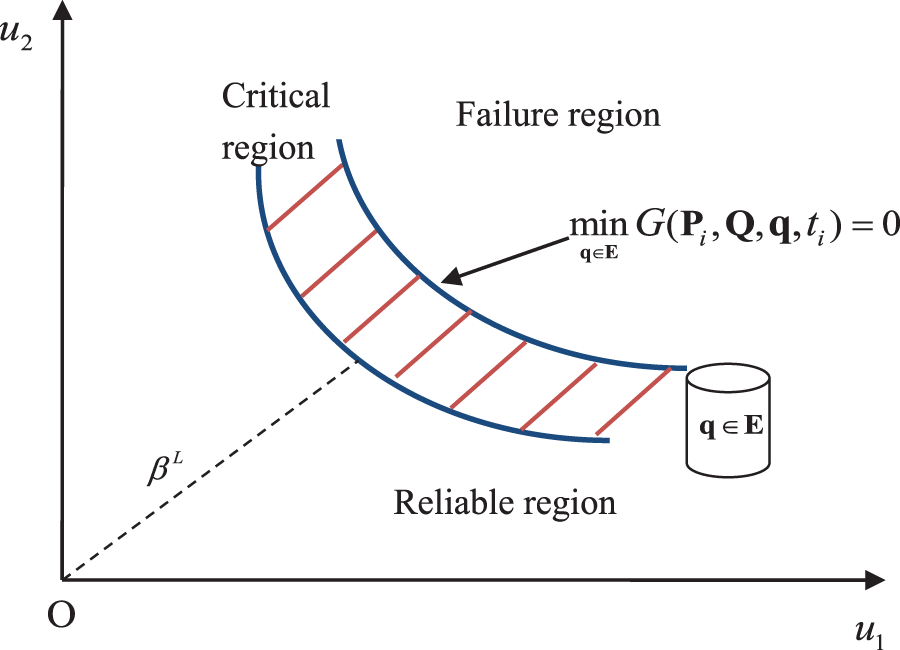
Figure 1: Limit-state strip caused by convex variables

The solution to Eq. (15) yields an most probable point (MPP) (P¯i,Q¯); q~ is the most disadvantageous point (MDP), and it represents an optimal solution to the following optimization problem:

minqG(Pi,Q,q,ti)s.t. qiTqi≤1(i=1,2,…,e)(16)

The hybrid reliability index is defined by Eqs. (15) and (16), which are formulated as nested optimization problems. The outer layer aims to search for the MPP (P¯i,Q¯), while the inner layer focuses on locating the MDP q~. However, it is a challenge to solve the above-mentioned nested optimization problem. Therefore, it is necessary to develop an efficient decoupling algorithm.

4  Proposed Analysis Method of Structural Time-Variant Reliability with Random and Uncertain-But-Bounded Variables

4.1 Establishment of an Equivalent Model

The time-variant reliability analysis based on the probability and ellipsoid model can be mathematically expressed in the form of Eq. (15) using normalized normal random and uncertain-but-bounded variables.

Random variables Pi,Q are retained, whereas an uncertain-but-bounded variable q becomes an independent random variable; namely, a non-probabilistic standardized variable is transformed into a random variable subjected to a uniform distribution, which can be expressed as follows:

qi∼u(qiL,qiR),i=1,2,…,e(17)

qi∈E,i=1,2,…,e(18)

where qiL and qiR are the lower and upper bounds of qi, respectively.

The ith original ellipsoid model in Eq. (17) is transformed into a unit model using spherical coordinate transformation as follows:

qi,1<ρicos⁡αi1qi,2<ρisin⁡αi1cos⁡αi2⋮qi,ni−1<ρisin⁡αi1sin⁡αi2sin⁡αi3⋯sin⁡αi,ni−2cos⁡αi,ni−1qi,ni<ρisin⁡αi1sin⁡αi2sin⁡αi3⋯sin⁡αi,ni−2sin⁡αi,ni−1(19)

with qi,ni as the nth component of qi, the uncertain space of Eq. (17) becomes:

Δi={(ρi,αij)|ρi∈[0,1],αij∈[0,2π],i=1,2,…,e;j=1,2,…,ni−1}(20)

where ρi is the radical coordinate and αi,j is the jth angular coordinate for the ith ellipsoid.

For the convex set of hype ellipsoids, uniformly distributed random numbers need to be generated in the ellipsoid body, which is equivalent to performing the uniform sampling in the unit hypersphere in each Q space, that is, ρi∈[0,1], αij∈[0,2π], which can be expressed as follows:

ρi∼u(ρiL,ρiR)=u(−1,1),i=1,2,…,e(21)

αij∼u(αijL,αijR)=u(0,2π),i=1,2,…,e(22)

where ρiL and ρiR are the lower and upper bounds of ρi, respectively; αijL and αijR are the lower and upper bounds of αij, respectively; u(⋅) represents the uniform distribution.

After substituting variables u = [P,Q] and τ=[ρ,α] into Eq. (15), a reliability problem with mixed variables can be expressed by:

{ βL=minu,τ‖ u ‖2+‖ τ ‖2s.t. G′(u,τ,ti)=0,i=1,2,…,m    τL≤τ≤τR(23)

where G′ represents the transformed limit state function in standard space; τL and τR are the lower and upper bounds of τ, respectively.

4.2 Model Equivalence Proof

By solving Eq. (23), MPP (u¯,τ~) can be obtained. According to the related literature [39,40], the MPP demonstrates the highest level of probability density in comparison to all other points on the limit state function. Therefore, the point (u¯,τ~) represents the solution to the following problem:

{maxu,τfu,τ(u,τ)s.t.g(u,τ,ti)=0,i=1,2,…,m τL≤τ≤τR(24)

fu,τ(u,τ) is the probability density function of the random variables u and τ.

The above-presented optimization problem can be further written as:

{maxu,τfu(u)fτ(τ)s.t.g(u,τ,ti)=0τL≤τ≤τR(25)

Since τ is uniformly distributed, fτ(τ) is constant, so Eq. (25) becomes:

{maxu,τfu(u)s.t.g(u,τ,ti)=0,i=1,2,…,mτL≤τ≤τR(26)

Eq. (26) is an optimization problem with constraints. Based on the KKT (Karush-Kuhn-Tucker) conditions, it can be written that:

{−∇ukfX(u)+λ1∇ukg(u,τ,ti)=0,k=1,2,…,nλ1∇τjg(u,τ,ti)+λ3j−λ2j=0,j=1,2,…,eλ2j(τjL−τj)=0,j=1,2,…,eλ3j(τj−τjR)=0,j=1,2,…,eg(u,τ,ti)=0,i=1,2,…,mτjL≤τj≤τjR,j=1,2,…,e(27)

where λ1, λ2j, λ3j represent Lagrange multipliers.

According to Eq. (15), the MPP point is the solution to the following optimization problems:

{maxufu(u)s.t.minτg(u,τ,ti)=0τL≤τ≤τR(28)

The constraint in Eq. (28) has a suboptimization problem, which satisfies the following KKT necessary conditions:

{∇τig(u,τ,ti)+λ3j−λ2j=0,j=1,2,…,nλ2i(τjL−τj)=0,j=1,2,…,nλ3i(τj−τjR)=0,j=1,2,…,nτjL≤τj≤τjR,j=1,2,…,e(29)

The following expression can be derived by substituting Eq. (29) into Eq. (28):

{maxufu(u)s.t.g(u,τ,ti)=0,j=1,2,…,e∇τig(u,τ,ti)+λ3i−λ2i=0,i=1,2,…,nλ2i(τjL−τj)=0,i=1,2,…,nλ3i(τj−τjR)=0,i=1,2,…,nτjL≤τj≤τjR,j=1,2,…,e(30)

It can be noticed that Eqs. (30) and (27) have the same expression, which mathematically proves that the current equivalent model has the same solution as the original model.

4.3 Linearization of the Limit-State Equation

The limit state function is initially linearized at the MPP to simplify calculations since Eq. (15) incorporates multiple limit state equations. Consequently, Eq. (15) undergoes a transformation as follows:

Ps(T)={∩i=1m[∑j=1n∂Gi∂Pi,j|P¯i,j(Pi,j−P¯i,j)+∑k=1h∂Gi∂Qk|Q¯i,k(Qk−Q¯i,k)+∑l=1n∂Gi∂τl|τ~i,l(τl−τ~i,l)>0]}(31)

where P¯i,j, Q¯k, and τ~l can be obtained from the MPP in the standard space.

Then, Eq. (31) is transformed into:

Ps(T)={∩i=1m[∑j=1n∂Gi∂Pi,j|P¯i,j(−P¯i,j)+∑k=1h∂Gi∂Qk|Q¯i,k(Qk−Q¯i,k)+∑l=1n∂Gi∂τl|τ~i,l(τl−τ~i,l)>−∑j=1n∂Gi∂Pi,j|P¯i,jPi,j]}(32)

Next, define a new random vector ξi as follows:

ξi=−∑j=1n∂Gi∂Pi,j|P¯i,jPi,j,i=1,2,⋯,m(33)

Considering that Pi,j is a random variable following the normal distribution with a standard deviation, it can be deduced that vector ξi also conforms to the normal distribution in m dimensions.

Based on the characteristics of a random vector’s mean vector and covariance matrix, the mean vector μξ and covariance matrix Cξ can be respectively expressed as follows:

(μξ)i=−∑j=1n∂Gi∂Pi,j|P¯i,j μPi,j=0,i=1,2,⋯,m(34)

(Cξ)i,v=∑k=1n∑j=1n∂Gi′∂Pi,j|P¯i,j∂Gv′∂Pv,k|P¯v,kCP((i−1)n+j,(v−1)n+k),i,v=1,2,…,m(35)

The construction of matrix C is explained in detail in [22]. Combined with the m-dimensional normal distribution function, Eq. (35) can be further transformed into:

Ps(T)=∫0+∞∫0+∞⋯∫0+∞ϕm{[∑j=1n∂Gi∂Pi,j|P¯i,j(−P¯i,j)+∑k=1h∂Gi∂Qk|Q¯i,k(Qk−Q¯i,k)+∑l=1n∂Gi∂τl|τ~i,l(τl−τ~i,l)],μθ,Cθ}×fQ(Q)dQ(36)

The problem defined in the above expression is a multivariate integral problem, and a large number of complex operations need to be performed during its numerical calculation. Therefore, a new random variable E is introduced to transform Eq. (36) into:

Ps(T)=∬⋯∫ΩfE(e)fQ(Q)dQde=Prob{FE−1{ϕm{[∑j=1n∂Gi∂Pi,j|P¯i,j(−P¯i,j)+∑k=1h∂Gi∂Qk|Q¯i,k(Qk−Q¯i,k)+∑l=1n∂Gi∂τl|τ~i,l(τl−τ~i,l)],μθ,Cθ}}−E>0}(37)

where Ω denotes the integral boundary, and it is defined by:

Ω={E,Q|E<FE−1{ϕm{[∑j=1n∂Gi∂Pi,j|P¯i,j(−P¯i,j)+∑k=1h∂Gi∂Qk|Q¯i,k(Qk−Q¯i,k)+∑l=1n∂Gi∂τl|τ~i,l(τl−τ~i,l)],μθ,Cθ}}}(38)

where FE′−1(⋅) is the inverse function of FE′(⋅).

Thus, a new function can be defined as follows:

G′(E,τ)=FE−1{ ϕm{ [ ∑j=1n∂Gi∂Pi,j|P¯i,j(−P¯i,j)+∑k=1h∂Gi∂Qk|Q¯i,k(Qk−Q¯i,k)                         +∑l=1n∂Gi∂τl|τ˜i,l(τl−τ˜i,l) ],μθ,Cθ } }−E(39)

The limit state function of the static reliability analysis model with mixed variables is expressed by Eq. (39). The traditional method can be effectively employed to solve the aforementioned equation. The final expression of the limit state equation is observed to be independent of the specific distribution of E. However, for computational convenience in practical engineering problems, it has been common practice to use the normal distribution.

4.4 Procedure

The following steps are to be implemented:

(1) Based on uncertainty information, identify three types of uncertainties in the limit state function as follows: random process variable, random variable, and non-probability variable. Next, input initial points P¯i,j0,Q¯i,k0, and τ~l0, and set the initial iteration number to K = 0;

(2) Discretize the stochastic process in the time-variant limit state function over different time periods and construct the reliability model based on the hybrid variables defined by Eq. (15);

(3) Standardize random variables, random processes, and non-probability variables; transform the non-probability variable into a random variable with uniform distribution;

(4) Design an equivalent model, as shown in Eq. (23), and obtain points P¯i,jK,Q¯i,kK, and τ~lK at each moment;

(5) Linearize the limited state function at points P¯i,jK, Q¯i,kK, and τ~lK, as shown in Eq. (31);

(6) Simplify the static reliability analysis model, as shown in Eq. (39); calculate the transformed reliability model by the FORM;

(7) If the MPP meets the convergence criteria, go to Step 8; otherwise, go to Step 4;

(8) Output P¯i,jK+1, Q¯i,kK+1, τ~lK+1, and β.

5  Numerical Examples

The effectiveness of the proposed method was verified by three numerical examples. To verify the accuracy and efficiency of the presented method, this study used the Monte Carlo (MC) method as a reference for each example. The Expansion Optimal Linear Estimation (EOLE) method was employed to generate random process samples. The sample number ns was set to 100,000.

5.1 Numerical Example 1

The time-variant limit state function was defined as follows:

g(x,a,Y(t),t)=a1a2−5(1+x4)+x1+4.6x2+4.6x3−0.025t+3(40)

where t is a time parameter with a variation range of 1–10.

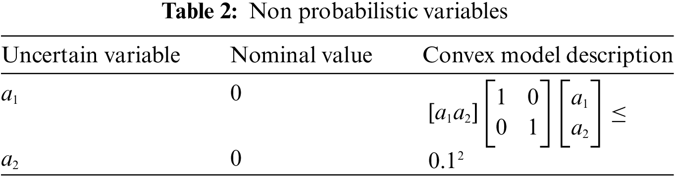
The distributions and values of non-probability parameter a of random parameters are shown in Tables 1 and 2, respectively.

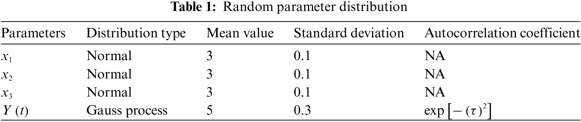
The comparison of the reliability index results of the proposed method and the Monte Carlo method are presented in Table 3 and Fig. 2. The reliability index values obtained by the proposed method were 1.97, 1.73, 1.55, 1.41, 1.29, 1.18, 1.08, 0.99, 0.90, and 0.83; the reliability index values obtained by the Monte Carlo method were 1.84, 1.62, 1.46, 1.34, 1.23, 1.14, 1.05, 0.98, 0.91, and 0.84. The reliability index decreased monotonously with time, which represented the fundamental difference between the time-variant reliability model and the static reliability model. The deviations between the proposed and Monte Carlo methods were 7.07, 6.79, 6.16, 5.22, 4.88, 3.51, 2.86, 1.02, 1.10, and 1.19, having a maximum deviation of only 7.07%. The results calculated by the proposed method were accurate. Regarding the computational efficiency, the Monte Carlo method called the limit-state 53,501,481 times, and the proposed method called the function only 320 times, which indicated the high efficiency of the proposed method.

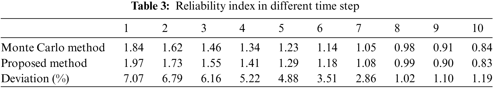
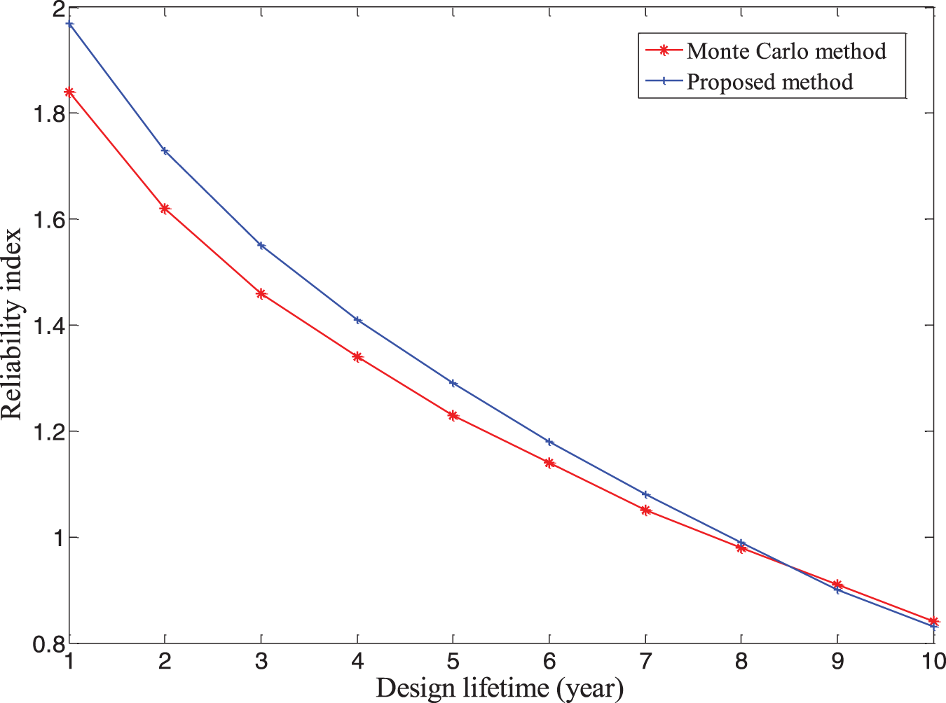
Figure 2: Variation curve of reliability index with time

5.2 Numerical Example 2

The second numerical example was a steel frame simply supported beam, as shown in Fig. 3 [18,22,41]. The cross-section had a rectangular shape with a width of b0 and a height of h0. A simply supported beam was subjected to a concentrated random load Q(t) at its midpoint in addition to a uniformly distributed load Q. The material density was ρ = 7.85 kN/m, and the uniformly distributed load was expressed as ρstb0h0; the yield strength of the material σ.

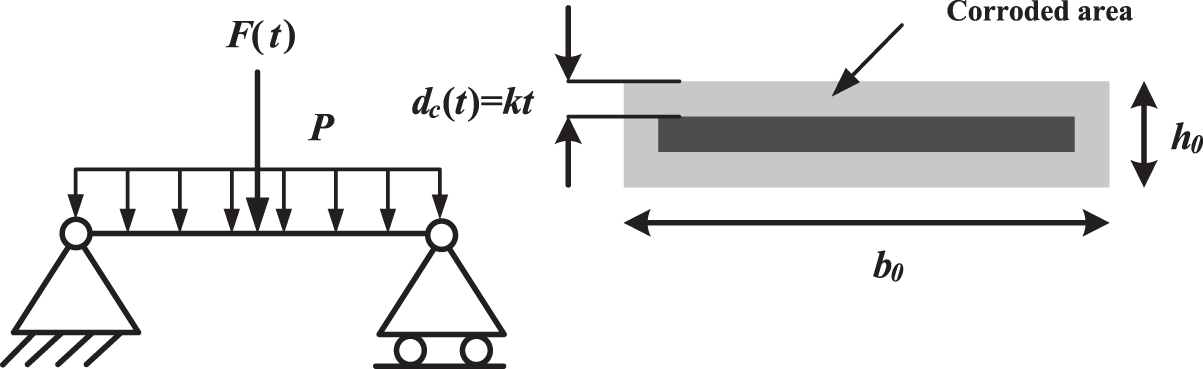
Figure 3: A simply supported steel beam structure [18,22,41]

Assuming that the simply supported beam was subjected to uniform linear corrosion in all directions during the service, and the corroded part completely lost its mechanical strength, the area of the uncorroded area could be expressed by:

A(t)=b(t)×h(t)(41)

where A(t) is the non-corroded area, having the width and height of b(t)=b0−κt and h(t)=h0−κt, respectively; κ is equal to 0.03 mm/year.

When the stress reached the ultimate stress of the material, the simply supported beam failed, and the limit state function was formulated as follows:

G(X,Y(t))=b(t)h2(t)4σ−(Q(t)L4+ρstb0h0L28)(42)

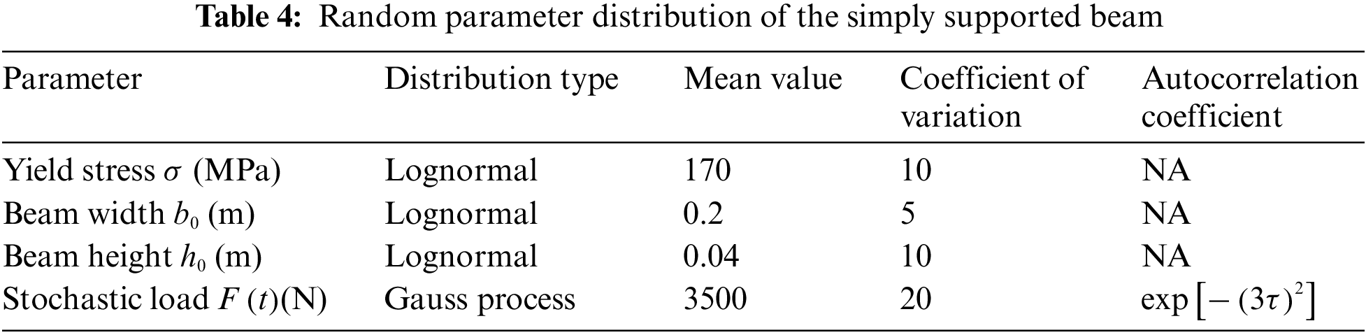
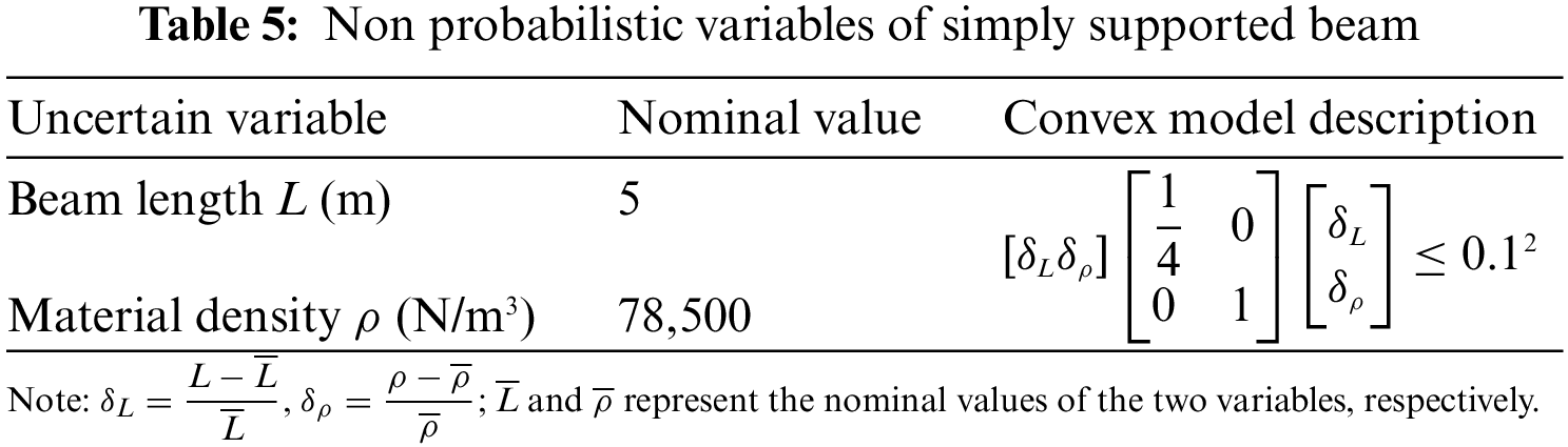
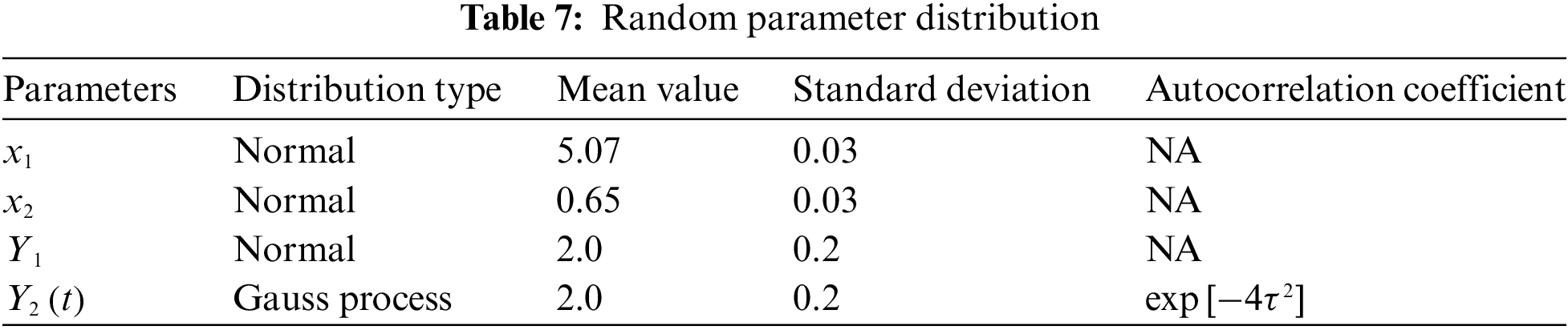
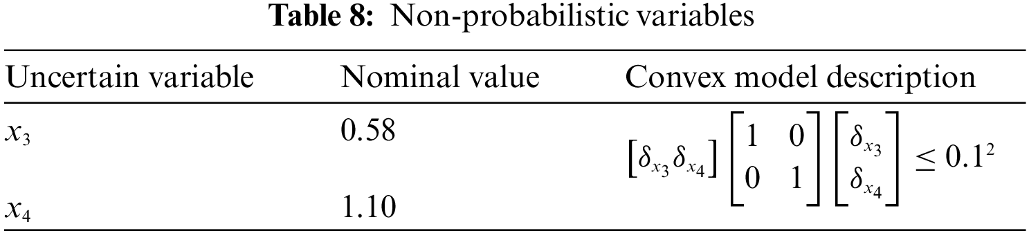
In this example, the random parameter distribution is presented in Table 4. The non probabilistic variables are shown in Table 5.

The reliability index results of the two methods are presented in Table 6, where it can be seen that the reliability indexes obtained by the proposed method were 2.73, 2.56, 2.46, 2.39, 2.33, 2.28, 2.24, 2.20, 2.17, and 2.14. Those obtained by the Monte Carlo method were 2.72, 2.55, 2.45, 2.37, 2.32, 2.27, 2.23, 2.19, 2.16, and 2.13, respectively. A similar conclusion could be drawn from the analysis of the results. As shown in Fig. 4, with the increase in the design service life, the reliability of the structure decreased continuously in the time-varying reliability analysis. The deviations between the two methods were 0.37%, 0.39%, 0.41%, 0.84%, 0.43%, 0.44%, 0.45%, 0.46%, 0.46%, and 0.47%. The time-varying reliability calculated by the proposed method was very close to the results obtained by the Monte Carlo method, and the error was within 0.84%, which indicated that the proposed method had sufficient accuracy. In terms of the calculation cost, the Monte Carlo method required the evaluation of the limit state function 59,433,341 times for each time-variant reliability analysis, whereas the proposed method performed only 2,792 evaluations, which clearly demonstrated that the proposed method had high calculation efficiency.

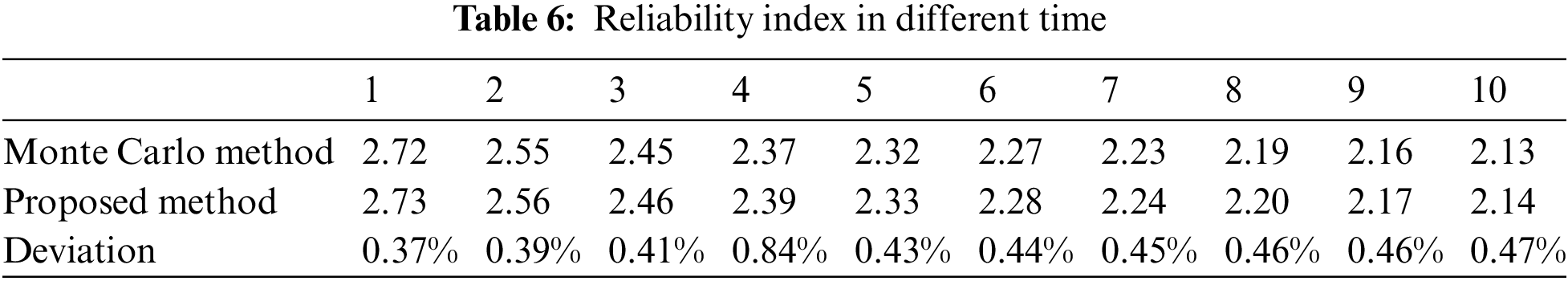
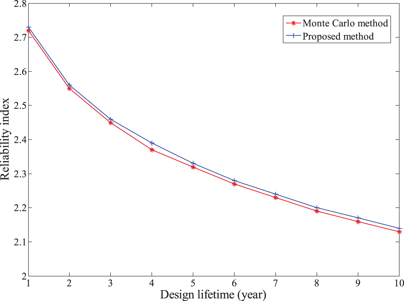
Figure 4: Variation curve of reliability index with time for simply supported beam

5.3 Reliability Prediction of Tablet Computer Structures

At present, electronic equipment has been widely used in industrial fields. A tablet computer is a quintessential consumer electronic device [36,42,43], and its Performance requirements such as high temperature environments, accidental drops, and operational safety have been usually considered. Therefore, it is necessary to analyze its reliability in the whole life cycle. The operational temperature of a tablet affects its working performance. In a high temperature environment, the operating temperature of the tablet used in this study was set at 45°C. The temperature TCH of a chip on the motherboard should not exceed its rated operating temperature T0CH = 65°C. As shown in Fig. 5, the tablet used in this experiment mainly consisted of a touch screen, a display screen, a battery, the mainboard, support, a front shell, and a back shell. The thickness of the front shell x1, the thickness of the touch screen x2, and the power consumption of the mainboard Y1 were treated as random variables.

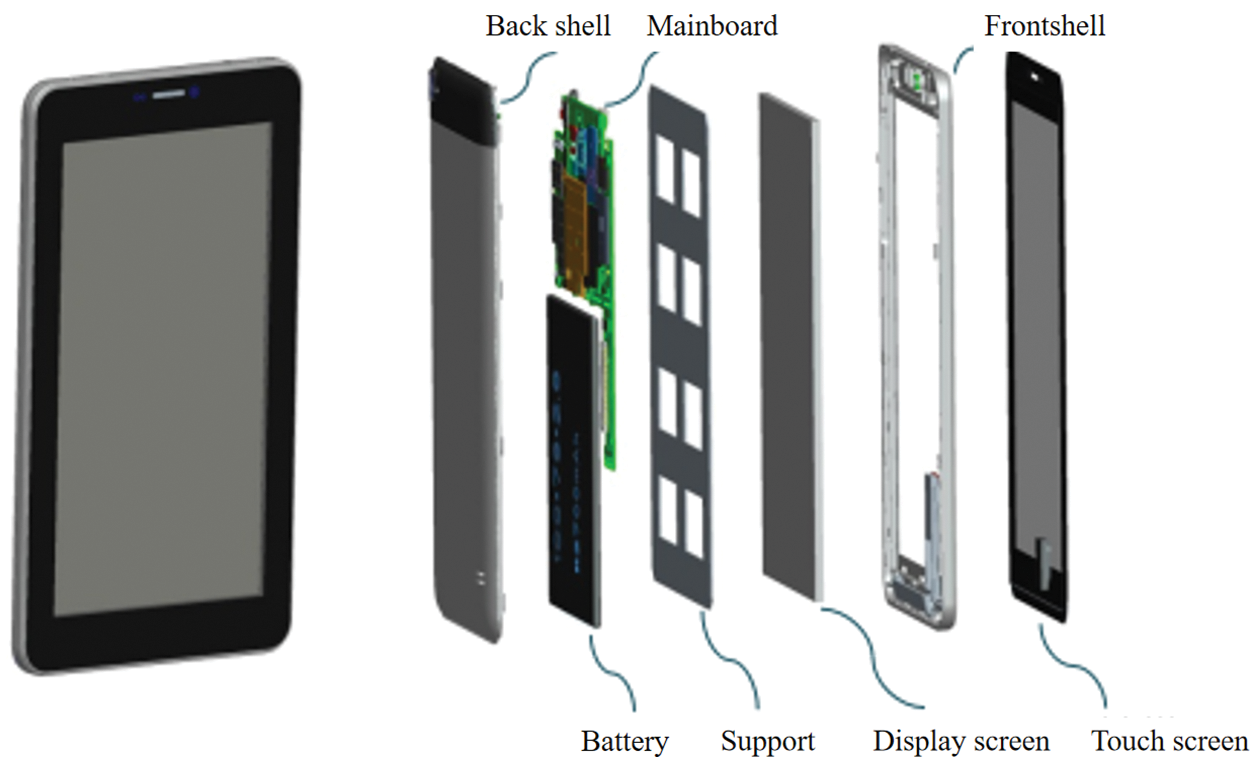
Figure 5: The structure of a tablet

The power consumption Y2(t) of the display screen was considered a stochastic process. The rated operating temperature decayed with time during service, and the decay function was defined by T0C=T0CHe−0.001t. The distribution parameters of random variables and processes are presented in Table 7. The thickness x3 of the support and the thickness x4 of the back shell were considered non-probabilistic variables, as shown in Table 8.

Thus, the reliability model of the actual problem could be constructed as follows:

g(t)=T0C−TCH(x1,x2,x3,x4,Y1,Y2(t))(43)

In the finite element analysis and calculation, 86,650 eight-node hexahedrons were used. To improve the calculation efficiency, the second-order response surface for TCH was constructed as follows [36,42]:

TCH(x1,x2,x3,x4,Y1,Y2(t))=−0.6330Y1(t)2+0.02776Y1(t)Y2(t)−0.2823Y1(t)X2+7.119Y1(t)+0.6486Y2(t)2−0.1774X12+1.767X1−0.03070X22−0.2237X32−0.1057X42+44.18(44)

In this example, the Monte Carlo method and the proposed method were used to conduct the time-varying reliability analysis. The analysis results are presented in Table 9 and Fig. 6, with a time step of 0.5 years. The tablet’s reliability changed over time and tended to decrease. As shown in Fig. 7, in the first year, the reliability index was 2.23, and the corresponding failure probability was 1.29 × 10−2; in the 10th year, the reliability index decreased to 1.20, and the corresponding failure probability was 1.15 × 10−1, which was more than eight times of the initial failure probability. Therefore, when designing a tablet computer, its performance in the whole life cycle should be considered, and a certain margin should be provided in the reliability design. The comparison results of the proposed method and the Monte Carlo method demonstrated that the proposed method was accurate, and the maximum deviation between the two methods was only 9.09%. In terms of the calculation cost, the proposed method called the performance function only 320 times.

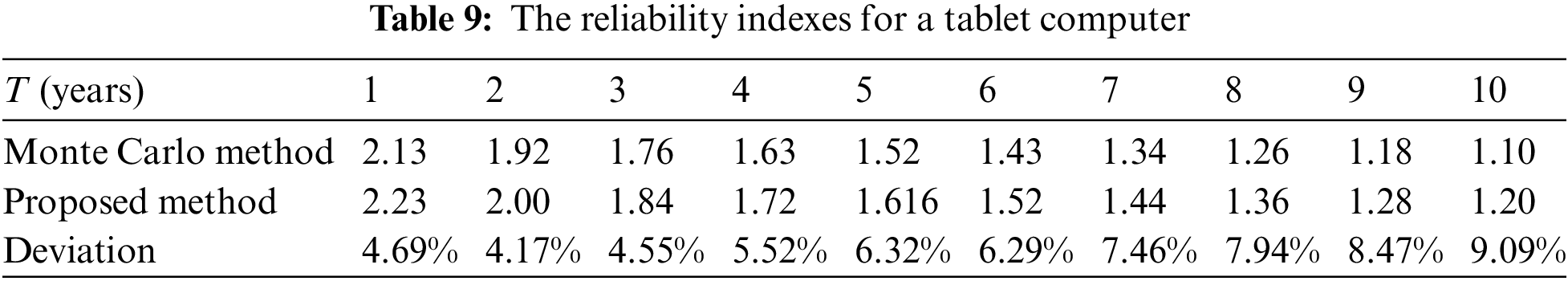
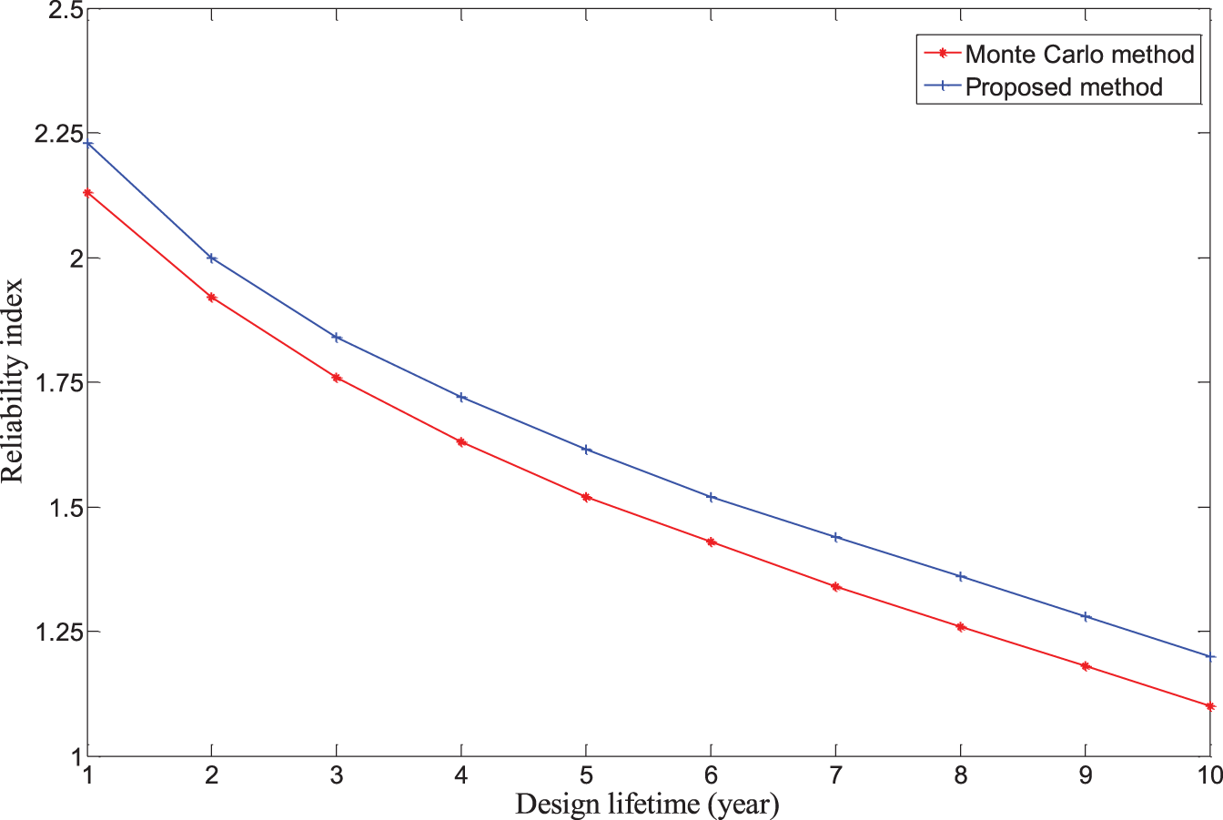
Figure 6: The reliability index over time for the structure of a tablet

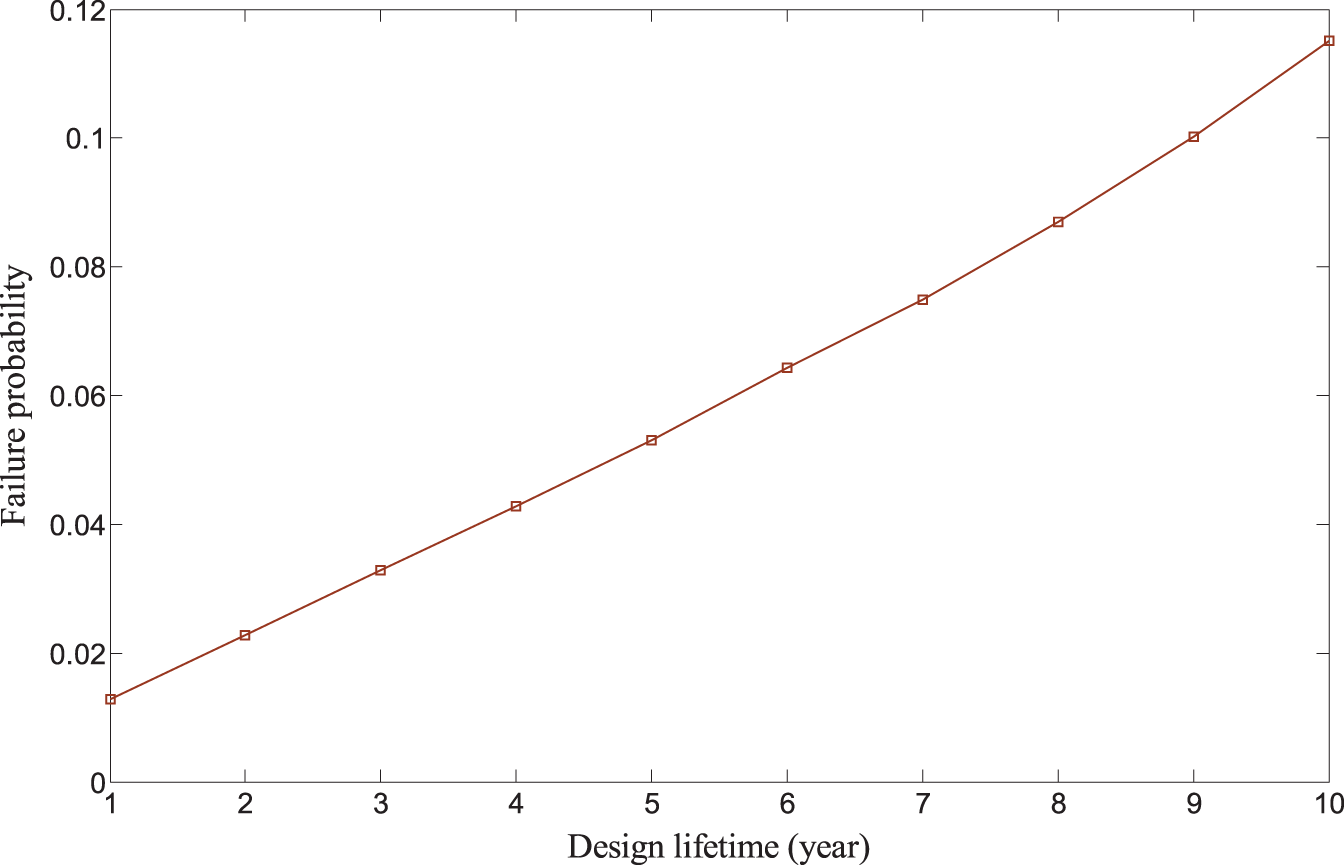
Figure 7: The failure probability for the structure of a tablet

6  Conclusion

This study proposes an innovative sequential iterative method to obtain the time-varying reliability index using a hybrid model that integrates the probabilistic and multi-ellipsoid convex models. The objective of this study is to solve a multi-layer nested optimization problem. The proposed method can solve the reliability problems when the resistance and load vary with time, and uncertain parameters have non-probabilistic uncertain parameters. The existing formulas and numerical techniques are used to develop a method for time-variant reliability assessment affected by random and bounded variations. Numerical examples show that the results of the proposed method are very close to those of the Monte Carlo method, but its computational efficiency is significantly improved. The structural analysis of the tablet shows that power degradation over time can decrease device reliability and, thus, should not be ignored in the device design process. The hybrid modeling theory can better evaluate the reliability of tablet computer structures when multiple sources of uncertain parameters are input. This study provides a complementary attempt for this field.

The decoupling framework has the limitation that it relies on gradient-based algorithms to solve the reliability problem, which requires small changes in variables between successive iterations to ensure the accuracy of the solution. Therefore, it is crucial to investigate robust algorithms for time variant reliability analysis to address significant fluctuations in variables. In addition, the adaptive surrogate model could be integrated into the decoupling framework to improve its efficiency, thus providing a potential approach to solve the problem of inefficiency in the reliability analysis of complex structures. Finally, future work could focus on developing advanced reliability analysis methods for time-dependent problems with high and strong nonlinearity.

Acknowledgement: Thank all the authors for their contributions to the paper.

Funding Statement: This work was partially supported by the National Natural Science Foundation of China (52375238), Science and Technology Program of Guangzhou (202201020213, 202201020193, 202201010399), and GZHU-HKUST Joint Research Fund (YH202109).

Author Contributions: The authors confirm contribution to the paper as follows: study conception and design: Fangyi Li; data collection: Fangyi Li, Dachang Zhu; analysis and interpretation of results: Huimin Shi, Dachang Zhu; manuscript writing: Fangyi Li, Dachang Zhu, Huimin Shi; manuscript review and editing: Fangyi Li. All authors reviewed the results and approved the final version of the manuscript.

Availability of Data and Materials: The authors do not have permission to share data.

Conflicts of Interest: The authors declare that they have no conflicts of interest to report regarding the present study.

References

1. Li, F., Liu, J., Wen, G., Rong, J. (2019). Extending SORA method for reliability-based design optimization using probability and convex set mixed models. Structural and Multidisciplinary Optimization, 59(4), 1163–1179. [Google Scholar]

2. Huang, Z. L., Jiang, C., Li, X. M., Wei, X. P., Fang, T. et al. (2017). A single-loop approach for time-variant reliability-based design optimization. IEEE Transactions on Reliability, 66(3), 651–661. [Google Scholar]

3. Li, F. Y., Wang, R. K., Zheng, Z. J., Liu, J. (2022). A time-variant reliability analysis framework for selective laser melting fabricated lattice structures probability and convex hybrid models. Virtual and Physical Prototyping, 17(4), 841–853. [Google Scholar]

4. Wen, G., Zhang, S., Wang, H., Wang, Z. P., He, J. et al. (2022). Origami-based acoustic metamaterial for tunable and broadband sound attenuation. International Journal of Mechanical Sciences, 239, 107872. [Google Scholar]

5. Wen, G., Chen, G., Long, K., Wang, X., Liu, J. et al. (2021). Stacked-origami mechanical metamaterial with tailored multistage stiffness. Materials & Design, 212, 110203. [Google Scholar]

6. Du, X. (2014). Time-dependent mechanism reliability analysis with envelope functions and first-order approximation. Journal of Mechanical Design, 136(8), 081010. [Google Scholar]

7. Rice, S. O. (1945). Mathematical analysis of random noise. The Bell System Technical Journal, 24(1), 46–156. [Google Scholar]

8. Sundar, V. S., Manohar, C. S. (2013). Time variant reliability model updating in instrumented dynamical systems based on Girsanov’s transformation. International Journal of Non-Linear Mechanics, 52, 32–40. [Google Scholar]

9. Breitung, K., Rackwitz, R. (1982). Nonlinear combination of load processes. Journal of Structural Mechanics, 10(2), 145–166. [Google Scholar]

10. Zayed, A., Garbatov, Y., Guedes Soares, C. (2013). Time variant reliability assessment of ship structures with fast integration techniques. Probabilistic Engineering Mechanics, 32, 93–102. [Google Scholar]

11. Andrieu-Renaud, C., Sudret, B., Lemaire, M. (2004). The PHI2 method: A way to compute time-variant reliability. Reliability Engineering & System Safety, 84(1), 75–86. [Google Scholar]

12. Sudret, B. (2008). Analytical derivation of the outcrossing rate in time-variant reliability problems. Structure and Infrastructure Engineering, 4(5), 353–362. [Google Scholar]

13. Wang, J., Gao, X., Cao, R., Sun, Z. (2021). A multilevel Monte Carlo method for performing time-variant reliability analysis. IEEE Access, 9, 31773–31781. [Google Scholar]

14. Wang, J., Cao, R. A., Sun, Z. L. (2021). Importance sampling for time-variant reliability analysis. IEEE Access, 9, 20933–20941. [Google Scholar]

15. Singh, A., Mourelatos, Z. P., Nikolaidis, E. (2011). An importance sampling approach for time-dependent reliability. Proceedings of the ASME International Design Engineering Technical Conferences and Computers and Information in Engineering Conference, 5, 1077–1088. [Google Scholar]

16. Li, H. S., Wang, T., Yuan, J. Y., Zhang, H. (2019). A sampling-based method for high-dimensional time-variant reliability analysis. Mechanical Systems and Signal Processing, 126, 505–520. [Google Scholar]

17. Du, W., Luo, Y., Wang, Y. (2019). Time-variant reliability analysis using the parallel subset simulation. Reliability Engineering & System Safety, 182, 250–257. [Google Scholar]

18. Zhang, D., Han, X., Jiang, C., Liu, J., Li, Q. (2017). Time-dependent reliability analysis through response surface method. Journal of Mechanical Design, 139(4), 041404. [Google Scholar]

19. Wang, Z., Wang, P. (2013). A new approach for reliability analysis with time-variant performance characteristics. Reliability Engineering & System Safety, 115, 70–81. [Google Scholar]

20. Hu, Y., Lu, Z., Wei, N., Zhou, C. (2020). A single-loop Kriging surrogate model method by considering the first failure instant for time-dependent reliability analysis and safety lifetime analysis. Mechanical Systems and Signal Processing, 145, 106963. [Google Scholar]

21. Hawchar, L., El Soueidy, C. P., Schoefs, F. (2017). Principal component analysis and polynomial chaos expansion for time-variant reliability problems. Reliability Engineering & System Safety, 167, 406–416. [Google Scholar]

22. Jiang, C., Huang, X., Han, X., Zhang, D. (2014). A time-variant reliability analysis method based on stochastic process discretization. Journal of Mechanical Design, 136(9), 091009. [Google Scholar]

23. Gong, J. X., Zhao, G. F. (1998). Reliability analysis for deteriortation structures. Journal of Build Structure, 19(5), 43–51 (In Chinese). [Google Scholar]

24. Jiang, C., Wei, X. P., Wu, B., Huang, Z. L. (2018). An improved TRPD method for time-variant reliability analysis. Structural and Multidisciplinary Optimization, 58(5), 1935–1946. [Google Scholar]

25. Ben-Haim, Y. (1994). A non-probabilistic concept of reliability. Structural Safety, 14(4), 227–245. [Google Scholar]

26. Muscolino, G., Santoro, R., Sofi, A. (2016). Reliability analysis of structures with interval uncertainties under stationary stochastic excitations. Computer Methods in Applied Mechanics and Engineering, 300, 47–69. [Google Scholar]

27. Jiang, C., Zhang, Q. F., Han, X., Liu, J., Hu, D. A. (2015). Multidimensional parallelepiped model—A new type of non-probabilistic convex model for structural uncertainty analysis. International Journal for Numerical Methods in Engineering, 103(1), 31–59. [Google Scholar]

28. Meng, Z., Zhang, Z., Zhou, H. (2020). A novel experimental data-driven exponential convex model for reliability assessment with uncertain-but-bounded parameters. Applied Mathematical Modelling, 77, 773–787. [Google Scholar]

29. Zhang, J., Xiao, M., Gao, L., Fu, J. (2018). A novel projection outline based active learning method and its combination with Kriging metamodel for hybrid reliability analysis with random and interval variables. Computer Methods in Applied Mechanics and Engineering, 341, 32–52. [Google Scholar]

30. Chen, N., Xia, S., Yu, D., Liu, J., Beer, M. (2019). Hybrid interval and random analysis for structural-acoustic systems including periodical composites and multi-scale bounded hybrid uncertain parameters. Mechanical Systems and Signal Processing, 115, 524–544. [Google Scholar]

31. Luo, Y., Kang, Z., Li, A. (2009). Structural reliability assessment based on probability and convex set mixed model. Computers & Structures, 87(21–22), 1408–1415. [Google Scholar]

32. Wang, C., Qiu, Z. P., Xu, M. H., Li, Y. L. (2017). Novel reliability-based optimization method for thermal structure with hybrid random, interval and fuzzy parameters. Applied Mathematical Modelling, 47, 573–586. [Google Scholar]

33. Guo, J., Du, X. (2009). Reliability sensitivity analysis with random and interval variables. International Journal for Numerical Methods in Engineering, 78(13), 1585–1617. [Google Scholar]

34. Li, F., Liu, J., Yan, Y., Rong, J., Yi, J. et al. (2020). A time-variant reliability analysis method for non-linear limit-state functions with the mixture of random and interval variables. Engineering Structures, 213, 110588. [Google Scholar]

35. Meng, Z., Guo, L., Hao, P., Liu, Z. (2021). On the use of probabilistic and non-probabilistic super parametric hybrid models for time-variant reliability analysis. Computer Methods in Applied Mechanics and Engineering, 386, 114113. [Google Scholar]

36. Shi, Y., Lu, Z. Z., Huang, Z. L. (2020). Time-dependent reliability-based design optimization with probabilistic and interval uncertainties. Applied Mathematical Modelling, 80, 268–289. [Google Scholar]

37. Liu, P. L., der Kiureghian, A. (1986). Multivariate distribution models with prescribed marginals and covariances. Probabilistic Engineering Mechanics, 1(2), 105–112. [Google Scholar]

38. Kang, Z., Luo, Y. J. (2010). Reliability-based structural optimization with probability and convex set hybrid models. Structural and Multidisciplinary Optimization, 42(1), 89–102. [Google Scholar]

39. Madsen, H. O. (1985). First order vs. second order reliability analysis of series structures. Structural Safety, 2(3), 207–214. [Google Scholar]

40. Breitung, K. (1989). Asymptotic approximations for probability integrals. Probabilistic Engineering Mechanics, 4(4), 187–190. [Google Scholar]

41. Ling, C., Lu, Z. (2020). Adaptive Kriging coupled with importance sampling strategies for time-variant hybrid reliability analysis. Applied Mathematical Modelling, 77, 1820–1841. [Google Scholar]

42. Liu, J., Chen, Z., Wen, G., He, J., Wang, H. et al. (2023). Origami chomper-based flexible gripper with superior gripping performances. Advanced Intelligent Systems, 5(10), 2300238. [Google Scholar]

43. Huang, Z. L., Jiang, C., Zhou, Y. S., Zheng, J., Long, X. Y. (2017). Reliability-based design optimization for problems with interval distribution parameters. Structural and Multidisciplinary Optimization, 55(2), 513–528. [Google Scholar]