
 Submit a Paper
 Propose a Special lssue
 Open Access
ARTICLE

Interaction Mechanisms between Natural Debris Flow and Rigid Barrier Deflectors: A New Perspective for Rational Design and Optimal Arrangement
1 Department of Geotechnical Engineering, College of Civil Engineering, Tongji University, Shanghai, 200092, China
2 Department of Hydraulic Engineering, College of Civil Engineering, Tongji University, Shanghai, 200092, China
* Corresponding Author: Dianlei Feng. Email:
(This article belongs to the Special Issue: Recent Advances in Computational Methods for Performance Assessment of Engineering Structures and Materials against Dynamic Loadings)
Computer Modeling in Engineering & Sciences 2024, 139(2), 1679-1699. https://doi.org/10.32604/cmes.2023.044094
Received 20 July 2023; Accepted 31 October 2023; Issue published 29 January 2024
 View Full Text
 Download PDF
Abstract
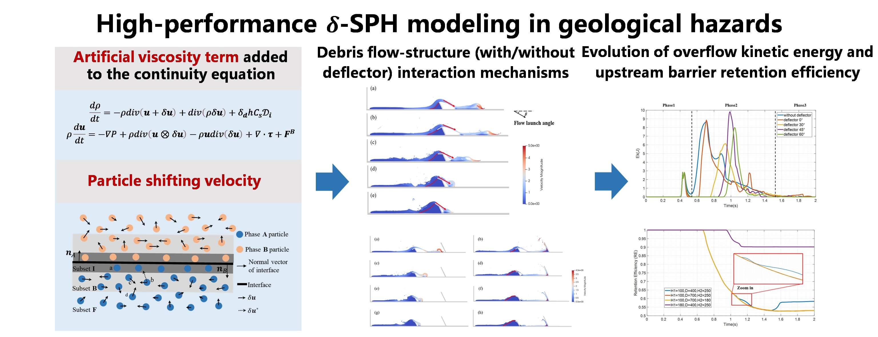
Rigid barrier deflectors can effectively prevent overspilling landslides, and can satisfy disaster prevention requirements. However, the mechanisms of interaction between natural granular flow and rigid barrier deflectors require further investigation. To date, few studies have investigated the impact of deflectors on controlling viscous debris flows for geological disaster prevention. To investigate the effect of rigid barrier deflectors on impact mechanisms, a numerical model using the smoothed particle hydrodynamics (SPH) method with the Herschel–Bulkley model is proposed to simulate the interaction between natural viscous flow and single/dual barriers with and without deflectors. This model was validated using laboratory flume test data from the literature. Then, the model was used to investigate the influence of the deflector angle and multi-barrier arrangements. The optimal configuration of multi-barriers was analyzed with consideration to the barrier height and distance between the barriers, because these metrics have a significant impact on the viscous flow pile-up, run-up, and overflow mechanisms. The investigation considered the energy dissipation process, retention efficiency, and dead-zone formation. Compared with bare barriers with similar geometric characteristics and spatial distribution, rigid barriers with deflectors exhibit superior effectiveness in preventing the overflow and overspilling of viscous debris flow. Recommendations for the rational design of deflectors and the optimal arrangement of multi-barriers are provided to mitigate geological disasters.Graphic Abstract
Keywords
Rigid barriers can effectively prevent natural hazards caused by mass-wasting debris flows in mountainous regions [1,2]. In large-scale natural debris flow disasters, bare barriers cannot retain flow material, and do not satisfy existing disaster protection requirements. Many design recommendations have been proposed to prevent debris flows from overflowing and overspilling [3,4]. For mitigation purposes, deflectors positioned atop the wall stem can redirect debris flows. The parapets in coastal structures are prototypes of these deflectors, and were initially designed to minimize water overspill and splash back [5,6]. The reduction factor quantifies the effectiveness of deflectors by measuring the discharge that overtops a barrier with a deflector in place and dividing this amount by the discharge that overtops a barrier without a deflector [7]. The comparison of bare barriers and rigid barriers with deflectors is shown in detail in Fig. 1, where
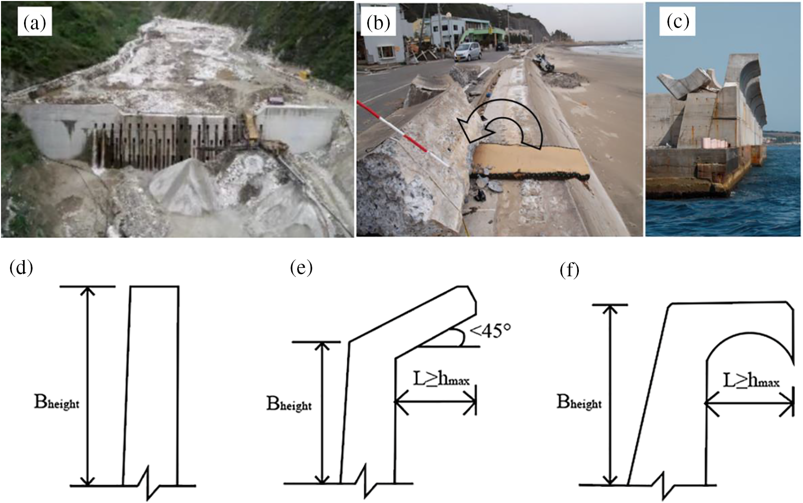
Figure 1: Countermeasures in hazard mitigation: (a) dredging of blocking structures in in the Qipan gully (China) [9]; (b) parapet failure in Toyoma Coast, Fukushima (Japan) [10]; (c) damages that occurred at Civitavecchia Port, Lazio, Italy [11]; (d) bare rigid barrier; (e) rigid barrier with inclined deflector; (f) rigid barrier with curved orthogonal deflector, modified from [8]
The interactions between debris flows and deflectors have been investigated using both physical and numerical models. Choi et al. [12] conducted preliminary small-scale flume experiments to investigate dry granular flow interaction with deflectors that had different angles. Ng et al. [4] conducted flume tests to investigate the flow kinematics of dry sand flows and the energy dissipation under the influence of deflectors. The results obtained by previous studies have revealed that conditions for adverse overflow strongly depend on the effective barrier height and length, and deflector angle. Notably, the flow characteristics of viscous debris flow differ significantly to those of dry granular flow, resulting in overspilling and hydrodynamic dead-zone formation [13–15]. Ng et al. [16] discussed the impact kinematics of fluids, including water and slurry, under different deflector geometries. A modified impact equation considering the flow-deflector interactions has been proposed. The impact, run-up, and pile-up mechanisms of saturated debris flow exhibit significant differences compared with those of dry granular flows in flow–barrier interactions. Consequently, research on the influence of deflectors on natural debris flow remains limited. Moreover, an appropriate constitutive model is required to capture the dynamic behavior of natural debris flow accurately and elucidate the flow–deflector interaction mechanisms.
Natural debris flow, which is a typical non-Newtonian fluid, has the characteristics of shear thinning or shear thickening behavior [17]. Various non-Newtonian rheological models, such as the Bingham model [18,19], power-law model [20], and Herschel–Bulkley model [21,22], have been proposed. Moreover, the constant threshold of yield stress (
The grid-based method and particle-based method are often used for modeling flow–structure interactions. For large-deformation debris flows, mesh-free methods can avoid the grid distortion in grid-based methods. Methods such as the discrete element method (DEM) [24], coupled computational fluid dynamics and discrete element method (CFD-DEM) [25], material point method (MPM) [26], and smoothed particle hydrodynamics (SPH) [27] are typical particle-based methods for capturing the complicated flow–barrier interactions of classic geomechanical problems. Among them, the SPH method has many advantages in solving large deformation problems over traditional grid-based methods [24–26]. This method has become widespread owing to its accuracy and stability under complex boundary conditions for the quantitative analysis of the mechanisms of dynamic interaction between natural debris flows and rigid barriers [27–29]. Wang et al. [30] investigated the flow behavior of debris flows using SPH, focusing on the propagation analysis of debris flows in terms of run-out distance and flow velocity. Dai et al. [31] used SPH to investigate the interaction between debris flows and structures, and estimated the impact force. Sun et al. [32,33] proposed the particle shifting technique (PST) to maintain the numerical stability and accuracy of the δ-plus-SPH scheme. Notably, the δ-SPH scheme introduces an artificial diffusive term to improve the high-frequency noise in the pressure field. Relevant results have revealed that δ-plus-SPH is feasible and reliable for investigating the dynamic interaction between debris flows and structures.
This study developed a δ-plus-SPH method and used it to investigate the influence of deflectors on the dynamic behavior of viscous debris flow. The primary objective of this study was to investigate the influence of deflector angles on viscous debris flow in both single-barrier and dual-barrier systems. The presentation and validation of the numerical results are obtained by using the δ-plus-SPH model, followed by the discussion of energy dissipation process, retention efficiency, and run-up and overflow mechanisms of viscous debris flow in rigid barriers with and without deflectors.
In the domain of computational fluid dynamics, the SPH method has emerged as a prominent mesh-free Lagrangian approach [28]. Central to the SPH method is the utilization of kernel functions to compute particle interactions, ensuring both consistency and stability in the numerical representation. This subsection presents the fundamental principles and mathematical formulations of the SPH method. Each equation is systematically introduced, accompanied by a rigorous exposition of its derivation, underlying assumptions, and its role within the overarching SPH framework.
The governing equations (Eq. (1)) include the mass and momentum balance, and require numerical solutions.
Eq. (1) has the derivative form of density and velocity;
Recently, the SPH method has been widely used to simulate large-deformation natural debris flows, because it can capture free surfaces and large deformable geomaterial boundaries [34]. By using the SPH method, the governing equations can be efficiently solved. The physical properties carried by the arbitrarily distributed discrete particles of debris flow are based on the distributed particles within a smoothing length. The field function
where
In Eqs. (3) and (4),
In Eq. (5),
In this study, the particle shifting technique (PST) and
In two-dimensional problems, the coefficient of the viscous term
where
The PST method is used to avoid arbitrary particle configuration, and the shifting velocity
In Eq. (9),
In Eq. (11),
This study employed the generalized wall boundary method and 4th-order Runge–Kutta time-integration technique to model intricate geometries. Notably, dummy particles can be used to model the interactions between the fluid phase and a solid boundary [42].
2.2 Numerical Model Setup and Rheological Model
Because deflectors are an efficient debris flow deflection method, a previous study [12] conducted flume tests to investigate the influence of different rigid barrier deflector angles. The overflow mechanisms are characterized by viscous flow launching off ramp-like dead zones, launch length
The setup of the 3D numerical flume models of the single barrier with deflectors and dual-barrier system are illustrated in Figs. 2a and 2b, and the detailed geometry of the 2D dual-barrier system with deflectors is shown in Fig. 2c. A rigid barrier with a 65-mm-long deflector (

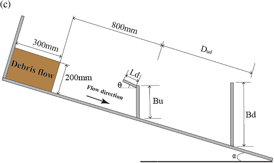
Figure 2: Numerical model setup: (a) 3D single barrier with deflectors; (b) 3D dual-barrier system; (c) 2D dual-barrier system with deflectors
The Herschel–Bulkley (HB) model was used to model the debris flow. The HB model has been widely used to investigate the rheological behavior of natural debris flow [47,48]. The deviatoric viscous stress tensor τ is expressed as follows:
In Eq. (12),
The apparent viscosity
The above model is singular in the static state when
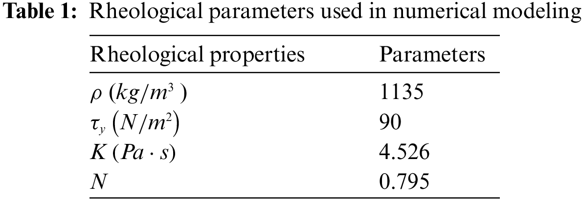
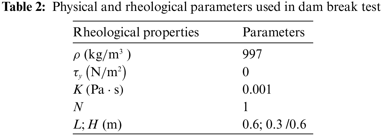
The dam break test reported by a previous study [50] was first used to calibrate the proposed numerical models. Fig. 3 shows the geometry of the dam break test and monitoring locations H1 and H4. Additionally, the physical and rheological parameters of the test fluid are listed in Table 2. As mentioned in the description of the rheological model in the Subsection 2.2, the debris flow viscosity is calculated by
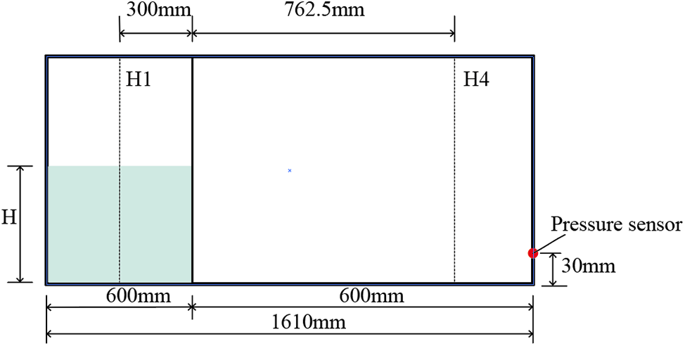
Figure 3: Dam break model test
The simulated results obtained by the proposed model were compared to the experimental results and are presented in Figs. 4 and 5. Fig. 4 mainly compares the relative flow elevation (
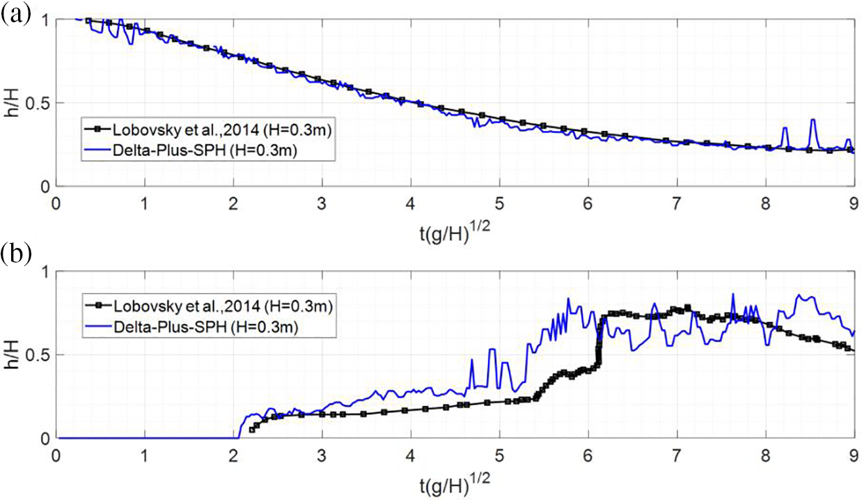
Figure 4: (a) Fluid level elevations at location H1 and (b) Fluid level elevations at location H4, compared with literature data [50]
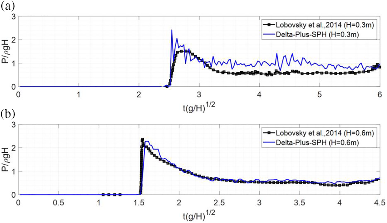
Figure 5: (a)
Unlike water, when a viscous debris flow collides with an obstacle, the flow velocity decreases dramatically, leading to an approximately triangular zone of a fluid at rest forming upstream of the obstacle. This deposited zone is referred to as a “dead zone” in mudflow [51]. The ensuing flow mounts this dead zone and expends part of its energy before hitting the barrier [1,24,52]. When the barrier’s retention capacity is reached, an overflow effect occurs: the debris flow material begins to escape from the barrier and flows forward through the barrier crest [53]. A dimensionless parameter
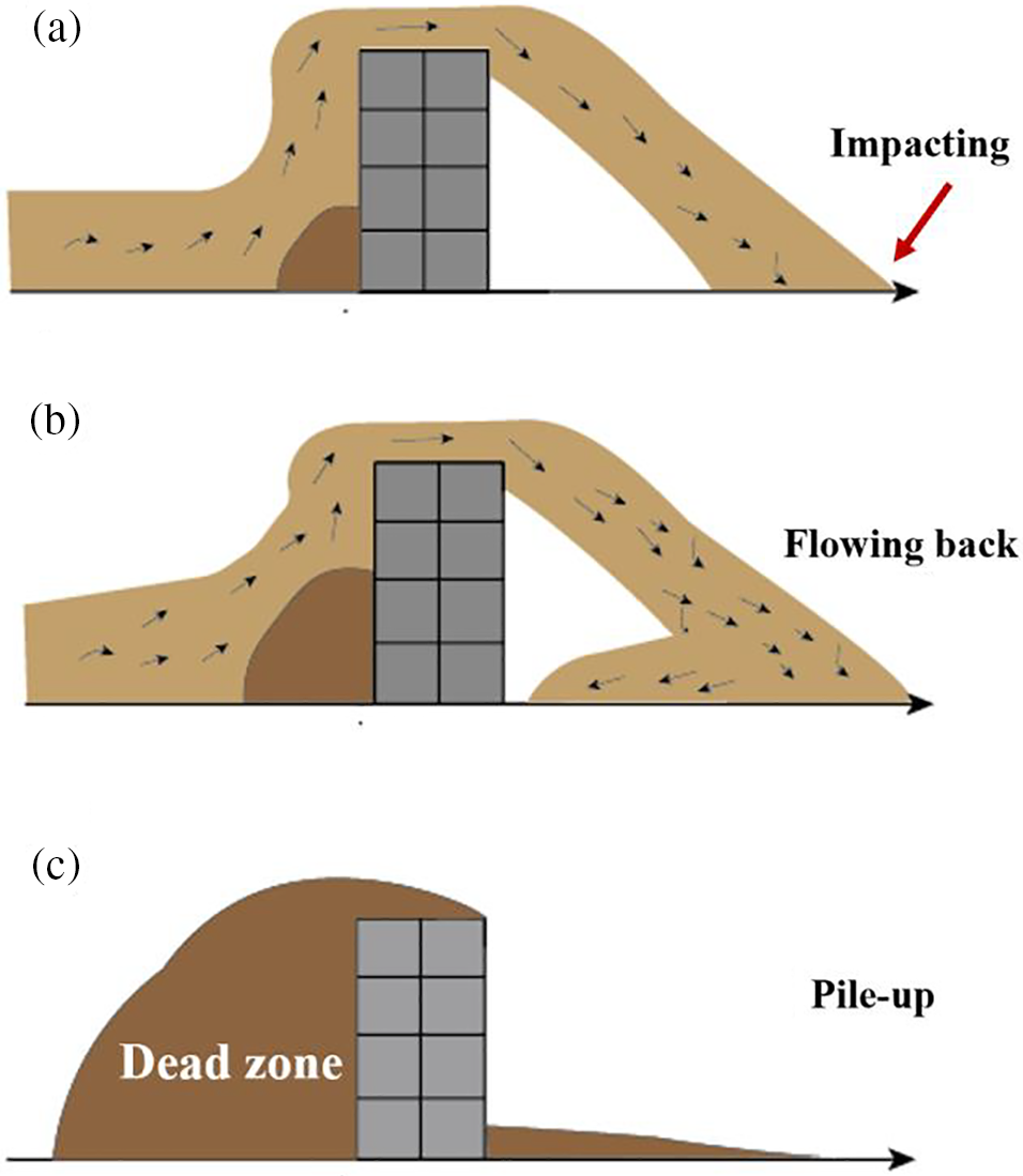
Figure 6: Schematic diagram of viscous debris overflow barrier (a) before and (b) after impact on flume base; (c) dead-zone formation
To gain a better understanding of the deflector’s robustness against disasters, the kinetic energy
Here,
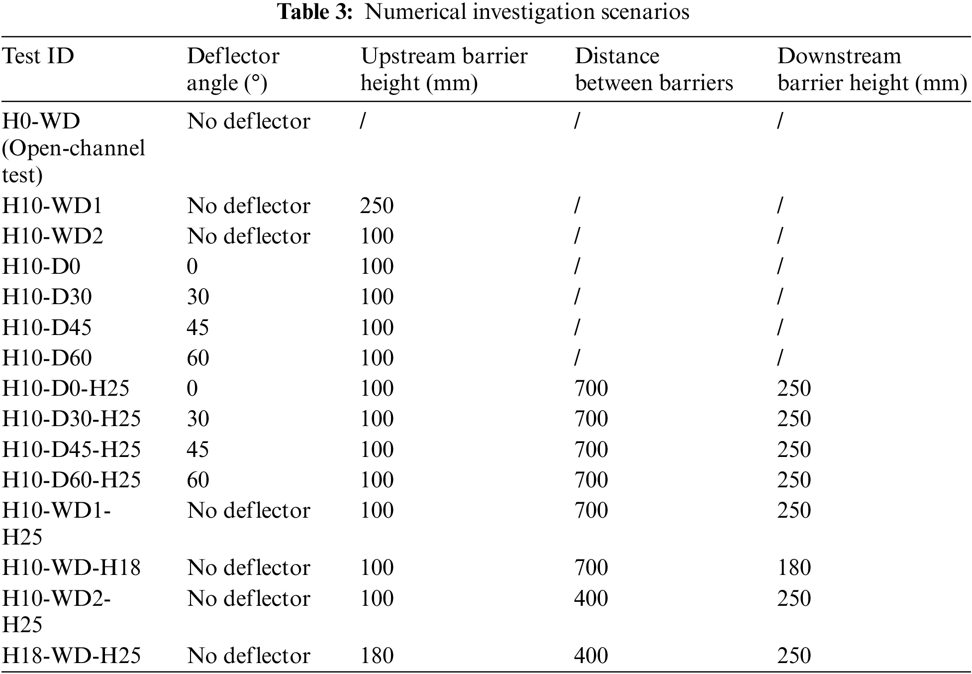
This study investigated the effect of single and dual-barrier systems with a deflector angle of 26° on viscous debris flow. To investigate the interaction between the viscous debris flow and the dual-barrier system, upstream and downstream barriers with different heights (
At the upstream barrier position, the flow thickness and front flow velocity were measured in the open-channel test (H0-WD) to calculate
Figure 7: Open-channel test (
Based on the simulation results, the rest of this paper focuses on the overflow pattern and pile-up mechanisms, and discusses the energy dissipation under the influence of the deflector angles, dead zone, and retention ability of the barrier with different barrier heights and location setups.
3.1 Overflow Pattern and Energy Dissipation
Fig. 8 illustrates the dynamic behavior of viscous flow overflow with and without deflectors. A single barrier with a height of 100 mm and deflector angles ranging from 0° to 60° was considered. Orthogonal deflectors (0°) and 30° deflectors caused the viscous flow to overflow the barrier quickly, resulting in higher velocity magnitude. The distance traveled by the overflow and its points of impact on the channel base are defined as the launch length (
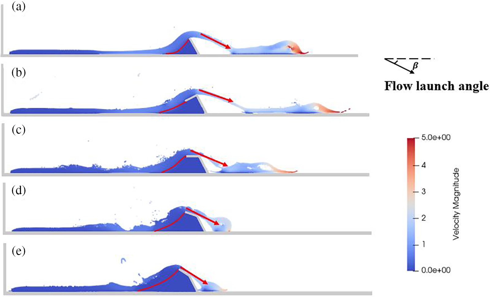
Figure 8: Overflow mechanisms: (a) without deflector (H10-WD2:
Deflectors with larger angles lead to a shorter launch length and larger launch angles when the viscous debris flow overflows the barrier and lands on the flume base. As shown in Fig. 9a, the launch length decreased from 1.845 to 1.273 m as the deflector angle increased from zero to 45°. However, the effect was less pronounced when the deflector angle exceeded 45°. The launch length of a barrier without deflectors (1.715 m) is marginally shorter compared with that of orthogonal deflectors (0°). The launch angle increased from approximately 20° to 35° as the deflector’s angles (ranging from 0° to 60°) increased (Fig. 9b).
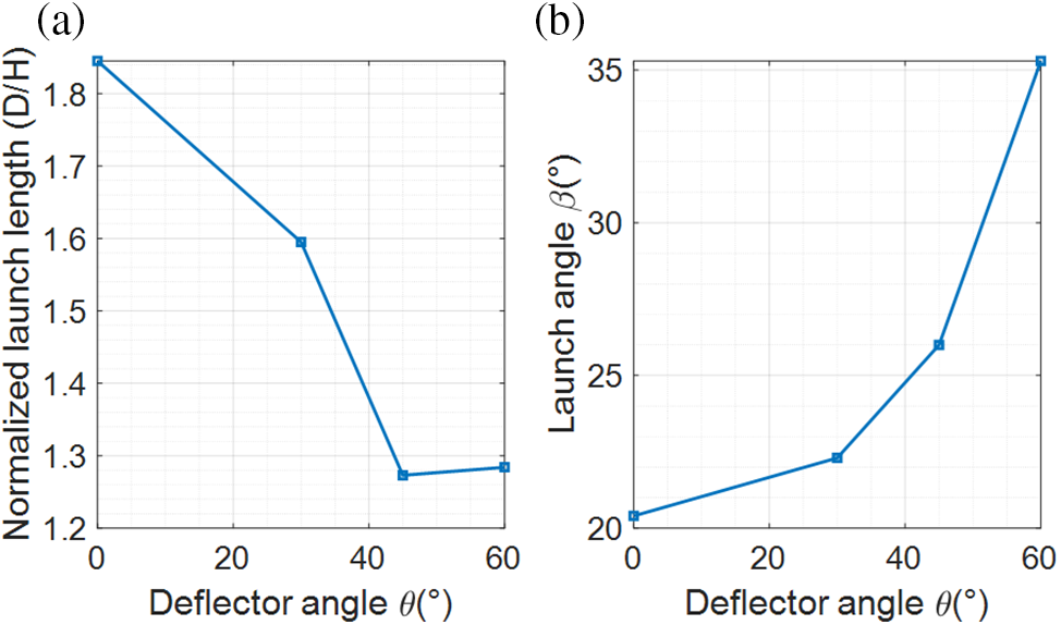
Figure 9: Influence of deflector angles on (a) launch length and (b) launch angle
In Fig. 10, the size of the dead-zone area markedly increases with the introduction of a barrier equipped with deflectors. Additionally, the dimensionless length of the dead-zone is positively correlated with the deflector angles. When the deflector angle exceeds 30°, the dimensionless length of the dead-zone increases significantly, reaching values above 3.5.
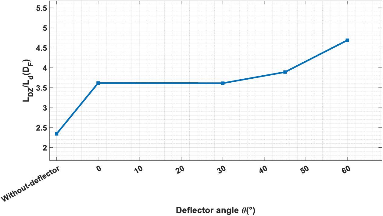
Figure 10: Influence of deflector angles on dimensionless length of dead-zone (
Fig. 11 illustrates the general evolution of overflow kinetic energy with various deflector angles, which can be categorized into three phases. Before impacting on the barrier, there is a kinetic energy peak in the process, owing to the acceleration of the debris flow. Phase 2 involves the dissipation process of the kinetic energy induced by the deflectors. Compared with barriers with deflectors, the kinetic energy of barriers without deflectors immediately increases, indicating a significant increase in the particle velocity. However, barriers with deflectors experience a period of zero kinetic energy when entering Phase 2 of dissipation, primarily because the deflectors directly intercept the impacting particles and then create a dead zone.
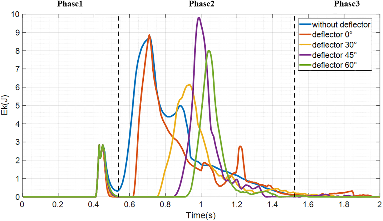
Figure 11: Evolution of overflow kinetic energy with different deflector angles
The overflow velocity magnitude and viscous debris direction are largely influenced by the deflector angles. The barrier with orthogonal deflectors exhibits a dissipation process similar to that of a barrier without a deflector, leading to the longest launch length. Although the 45° deflector significantly reduces the launch length, its capability of energy dissipation is inferior to that of the 60° and 30° deflectors within the monitored section. In the H10-D45 test program (Fig. 12), the dead zone starts to form when the flow impacts the barrier, and gradually grows and controls the overflow behavior observed around
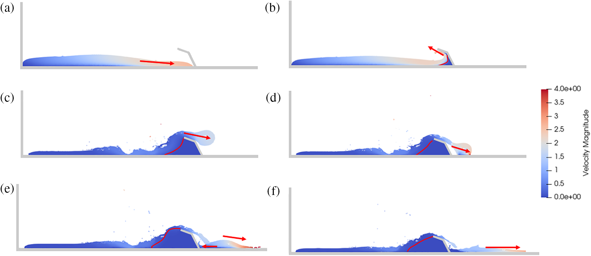
Figure 12: Flow–barrier interaction mechanisms under deflector angle
The energy dissipation of the dual-barrier system exhibits characteristics similar to the three stages observed in the single barrier structure described earlier (Fig. 13). The energy accumulation phase follows a pattern of initial increase and subsequent decrease. Compared with the upstream barrier with a height of 100 mm, the barrier with a height of 180 mm exhibits a zero-energy zone owing to the formation of a larger dead zone. The distance between barriers affects the energy dissipation process. A shorter distance results in a larger proportion of particles flowing back to the upstream barrier with higher velocity. In contrast, the downstream barrier with a height of 180 mm effectively intercepts the released viscous debris flow.
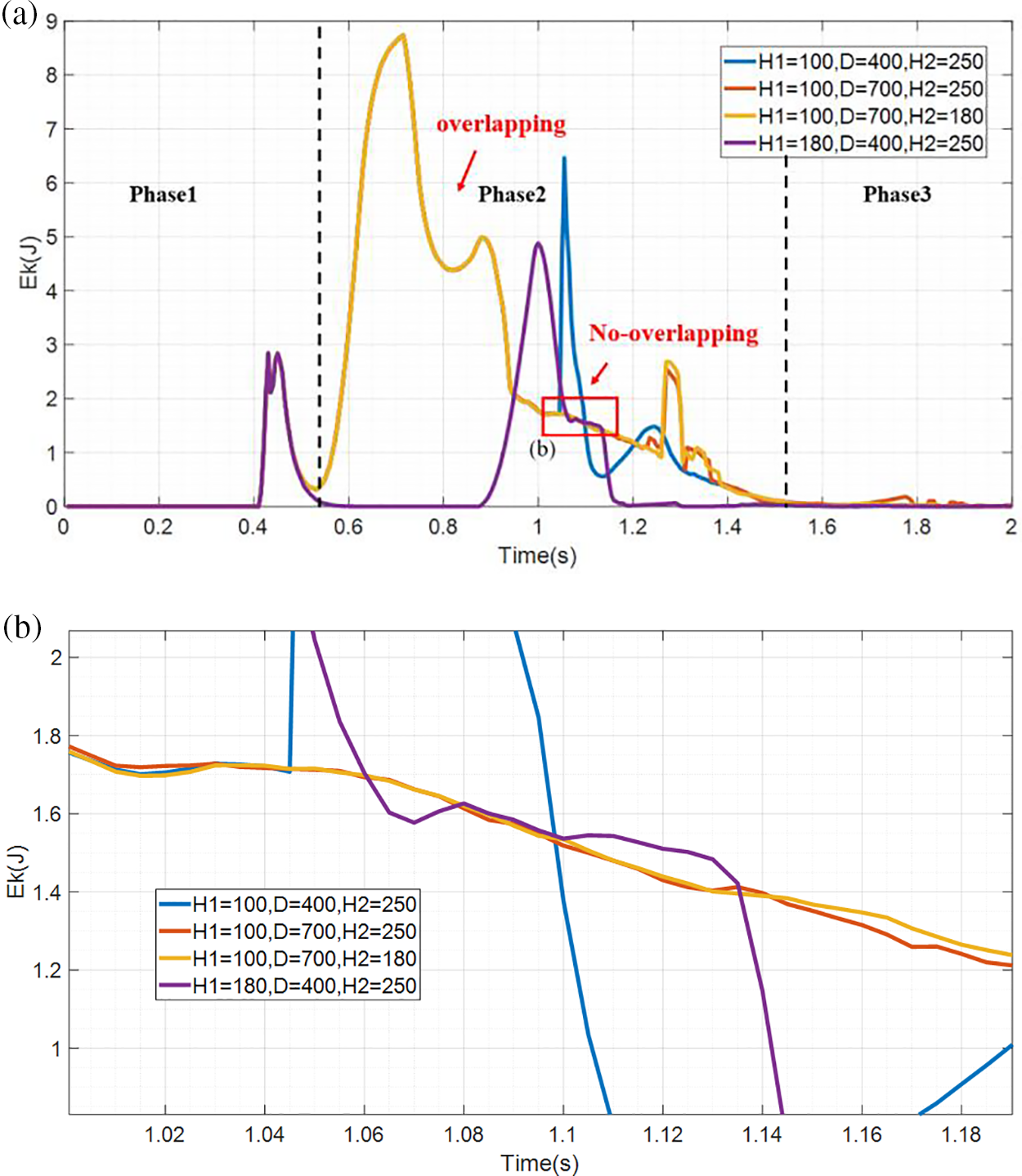
Figure 13: Evolution of overflow kinetic energy under different conditions of dual-barrier system: (a) global; (b) detail
3.2 Pile-Up Mechanism and Retention Efficiency
The barrier height, barrier location, and deflector angles greatly influence the control of the dynamic behavior of viscous flow. As shown in Fig. 14, increasing the height of a single barrier from 100 mm (
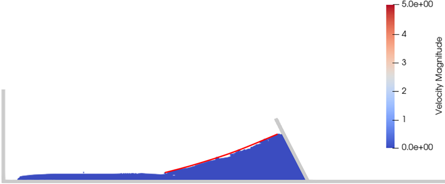
Figure 14: Pile-up mechanism of barrier with height of 250 mm (H10-WD1:
In this study, barriers with heights of 100 and 180 mm were investigated at distances of 400 and 700 mm, respectively. When the upstream barrier was equipped with deflectors, a downstream barrier height of 250 mm could intercept the entire debris volume in four test programs. The deflector angle influenced the formation of the dead zone near the deflectors, with larger angles resulting in more pronounced ramp-like dead zones. The results are presented in Fig. 15, illustrating that the dead zone serves as cushion layer at the upstream barrier. The impact of the overflowing debris flow on the downstream barrier results in the formation of dead zones with different sizes. Particularly, the upstream barrier equipped with an orthogonal deflector exhibits the highest momentum, leading to the rapid interception of viscous flow by the downstream barrier.
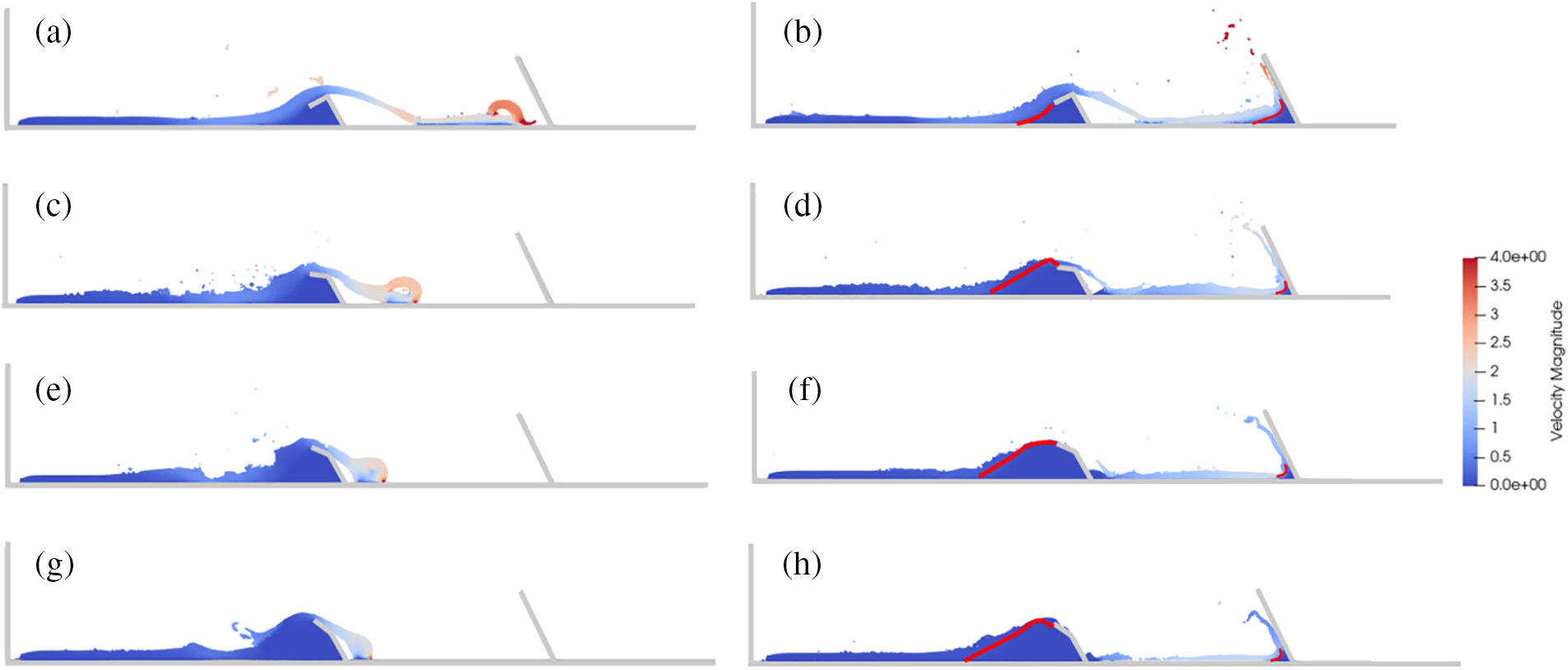
Figure 15: Pile-up mechanisms under influence of deflector angles: H10-D0-H25 (a)
Larger deflector angles can effectively retain a larger amount of debris flow. Fig. 16 shows that the deflector’s debris flow interception capability increases and then stabilizes starting from approximately 1.5 s. As shown in Fig. 17, when the deflector angle
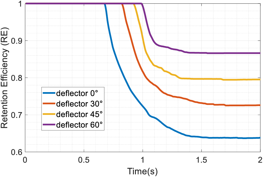
Figure 16: Time series of retention efficiency under influence of deflector angles
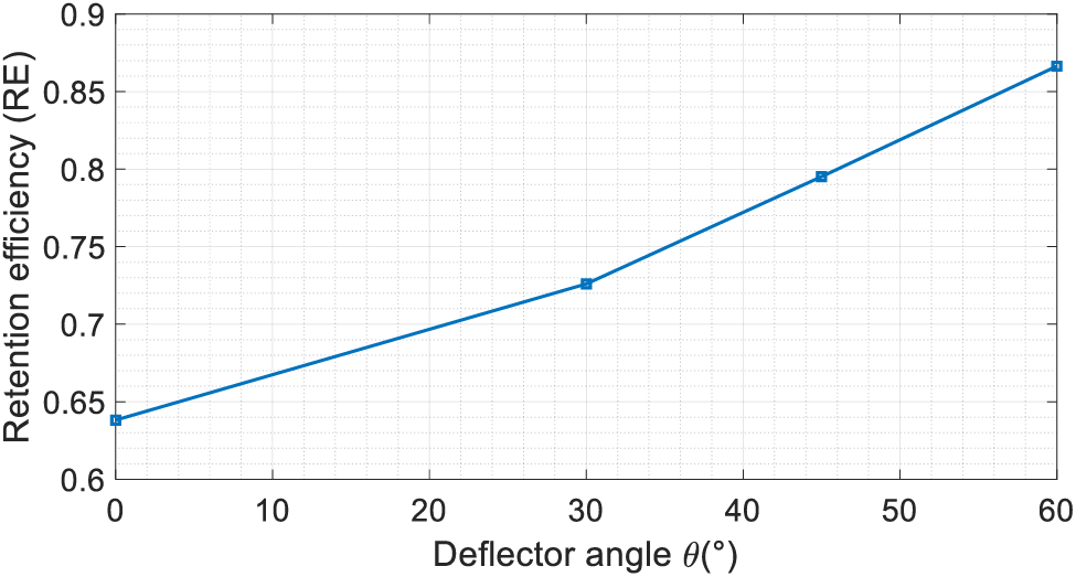
Figure 17: Influence of deflector angle on retention efficiency
In a dual-barrier system without deflectors, the ramp-like dead zones become steeper as the height of the upstream barrier increases (Fig. 18). Although the barrier distance is reduced by 42.9% to 300 mm, the downstream barrier retains the highest debris flow volume. Compared with the single barrier with retention efficiency (Fig. 19), the upstream barrier with a height of 180 mm intercepted over 90% of the debris flow, exceeding the interception of approximately 40% achieved by the upstream barrier with a height of 100 mm.
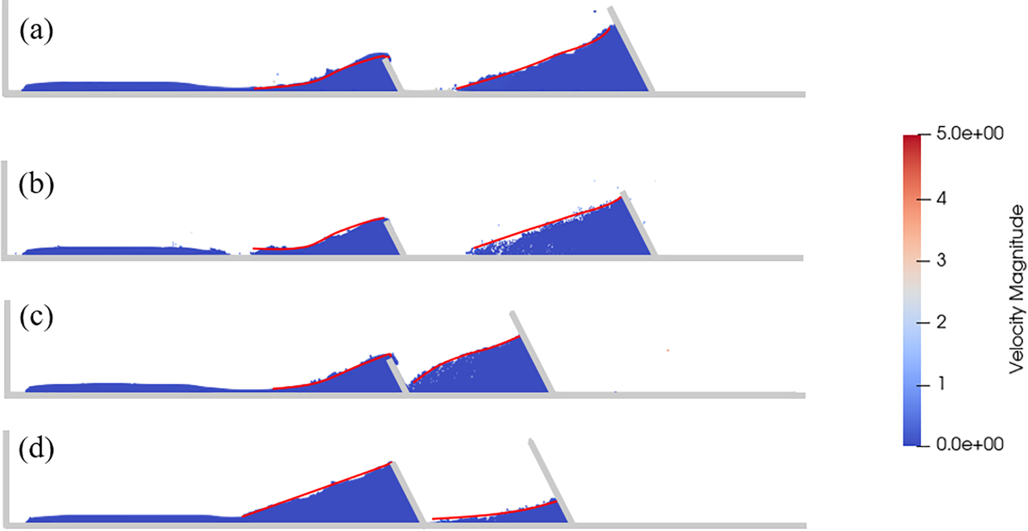
Figure 18: Pile-up mechanisms: (a) H10-WD-H25:
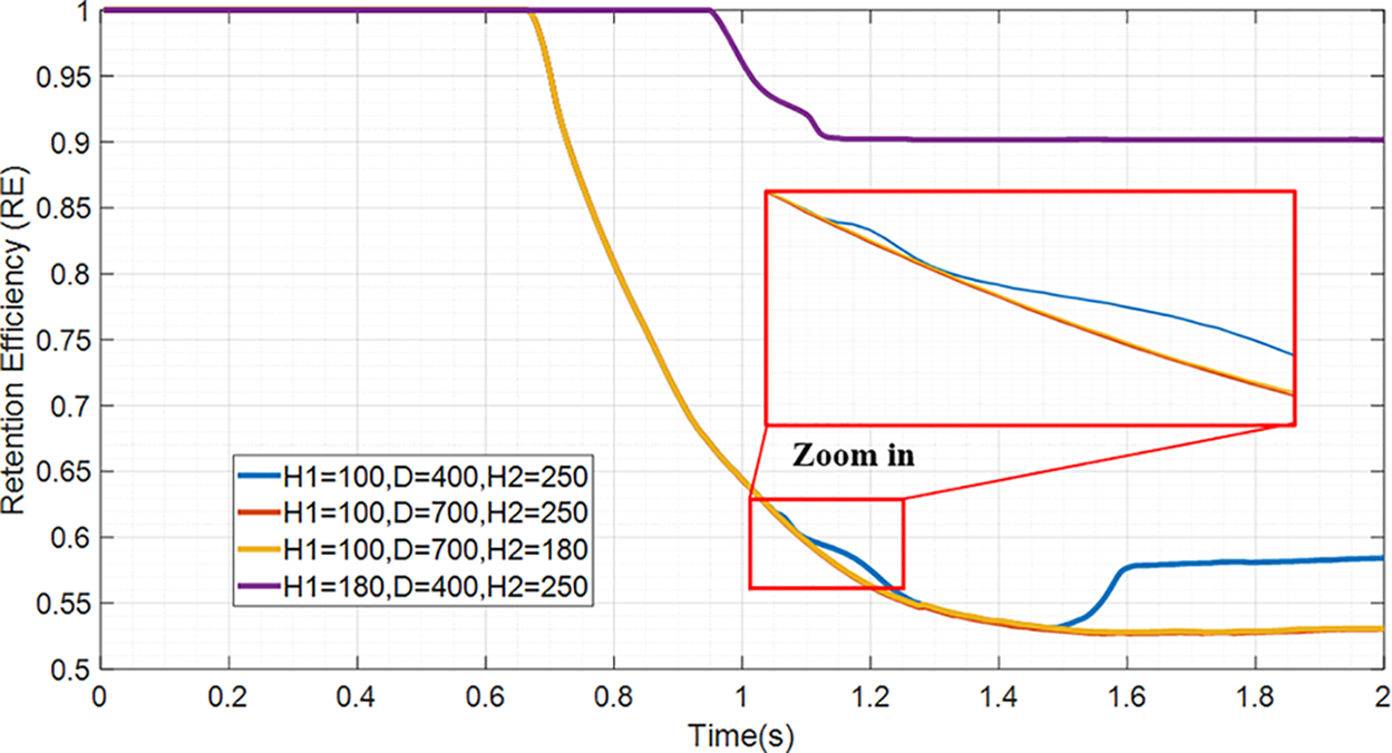
Figure 19: Time series of upstream barrier retention efficiency under different dual-barrier system conditions
This study investigated the interaction of viscous debris flow with barriers that have different deflector angles, and the impact of a dual-barrier system with different barrier heights and distances. The main conclusions are as follows:
(1) The interaction between viscous debris flows and barriers is largely determined by the deflector angles. Specifically, a deflector angle below 45° forms shallow ramp-like zones, promoting a thick and high-speed overflow downstream. The dimensionless length of the dead zone increases significantly when the deflector angle exceeds 30°. Moreover, the overflow mechanisms vary owing to the intricacies of viscous debris flows, with back-flows becoming more obvious when the flow velocity increases and the launch length decreases. There are three stages of energy in the dissipation process: the cumulative phase, interaction phase, and plateau phase.
(2) The barrier’s height and downstream positioning profoundly influence the effectiveness of single barriers in retaining flows. For instance, a barrier height decreasing from 250 to 180 mm cuts the retained flow volume by approximately one tenth, while a height reduction to 100 mm decreases the volume by approximately 40%. In dual-barrier systems, the spacing between the barriers also affects the dead-zone formation.
Although this study provides insights into the role of deflectors and dual-barrier systems against debris flows, further research into other influencing factors and the three-dimensional effects during viscous debris flow–structure interactions is required.
Acknowledgement: The authors thank the editor and the reviewers for their help to improve the quality of our manuscript.
Funding Statement: This study was supported by the National Natural Science Foundation of China (Grant Nos. 42120104008 and 42207198).
Author Contributions: Conceptualization, Y.H. and D.F.; methodology, B.L. and H.S.; formal analysis, B.L. and H.S.; investigation, B.L.; writing—original draft preparation, B.L.; writing—review and editing, Y.H. and D.F.; visualization, B.L.; supervision, D.F.; funding acquisition, Y.H. and D.F. All authors have read and agreed to the published version of the manuscript.
Availability of Data and Materials: The data sets used and analysed during this study are available from the corresponding author upon reasonable request.
Conflicts of Interest: The authors declare that they have no conflicts of interest to report regarding the present study.
References
1. Koo, R. C. H., Kwan, J. S. H., Ng, C. W. W., Lam, C., Choi, C. E. et al. (2017). Velocity attenuation of debris flows and a new momentum-based load model for rigid barriers. Landslides, 14(2), 617–629. [Google Scholar]
2. Pan, H., Wang, R., Huang, J., Ou, G. (2013). Study on the ultimate depth of scour pit downstream of debris flow sabo dam based on the energy method. Engineering Geology, 160, 103–109. [Google Scholar]
3. Hungr, O., Leroueil, S., Picarelli, L. (2014). The Varnes classification of landslide types, an update. Landslides, 11(2), 167–194. [Google Scholar]
4. Ng, C. W. W., Choi, C. E., Goodwin, S. R., Cheung, W. W. (2017). Interaction between dry granular flow and deflectors. Landslides, 14(4), 1375–1387. [Google Scholar]
5. Schoonees, T. (2014). Impermeable recurve seawalls to reduce wave overtopping (Ph.D. Thesis). Stellenbosch University. [Google Scholar]
6. Kortenhaus, A., Pearson, J., Bruce, T., Allsop, N. W. H., van der Meer, J. W. (2003). Influence of parapets and recurves on wave overtopping and wave loading of complex vertical walls. Coastal Structures, 2003, 369–381. [Google Scholar]
7. Verwaest, T., Vanpoucke, P., Willems, M., de Mulder, T. (2011). Waves overtopping a wide-crested dike. Coastal Engineering Proceedings, 1(32). [Google Scholar]
8. Kwan, J. S. H. (2012). Supplementary technical guidance on design of rigid debris-resisting barriers. Geotechnical Engineering Office, HKSAR. GEO Report, 270. [Google Scholar]
9. Su, N., Xu, L., Yang, B., Li, Y., Gu, F. (2023). Risk assessment of single-gully debris flow based on dynamic changes in provenance in the wenchuan earthquake zone: A case study of the qipan gully. Sustainability, 15(15), 12098. [Google Scholar]
10. Kato, F., Suwa, Y., Watanabe, K., Hatogai, S. (2012). Mechanisms of coastal dike failure induced by the Great East Japan Earthquake Tsunami. Coastal Engineering Proceedings, 1(33). [Google Scholar]
11. Castellino, M., Sammarco, P., Romano, A., Martinelli, L., Ruol, P. et al. (2018). Large impulsive forces on recurved parapets under non-breaking waves. A numerical study. Coastal Engineering, 136, 1–15. [Google Scholar]
12. Choi, C. E., Ng, C. W. W., Goodwin, S. R., Liu, L. H. D., Cheung, W. W. (2016). Flume investigation of the influence of rigid barrier deflector angle on dry granular overflow mechanisms. Canadian Geotechnical Journal, 53(10), 1751–1759. [Google Scholar]
13. Takahashi, T., Das, D. K. (2014). Debris flow: Mechanics, prediction and countermeasures, 2nd edition. UK:CRC Press. [Google Scholar]
14. Wang, T., Chen, X., Li, K., Chen, J., You, Y. (2018). Experimental study of viscous debris flow characteristics in drainage channel with oblique symmetrical sills. Engineering Geology, 233, 55–62. [Google Scholar]
15. Kong, Y., Zhao, J., Li, X. (2021). Hydrodynamic dead zone in multiphase geophysical flows impacting a rigid obstacle. Powder Technology, 386, 335–349. [Google Scholar]
16. Ng, C. W. W., Li, Z., Wang, Y. D., Liu, H., Poudyal, S. et al. (2023). Influence of deflector on the impact dynamics of debris flow against rigid barrier. Engineering Geology, 321, 107135. [Google Scholar]
17. Huang, X., García, M. H. (1998). A Herschel-Bulkley model for mud flow down a slope. Journal of Fluid Mechanics, 374, 305–333. [Google Scholar]
18. Schippa, L. (2020). Modeling the effect of sediment concentration on the flow-like behavior of natural debris flow. International Journal of Sediment Research, 35(4), 315–327. [Google Scholar]
19. Huang, Y., Jin, X., Ji, J. (2022). Effects of barrier stiffness on debris flow dynamic impact—II: Numerical simulation. Water, 14(2), 182. [Google Scholar]
20. Zanuttigh, B., Lamberti, A. (2007). Instability and surge development in debris flows. Reviews of Geophysics, 45(3), RG3006. [Google Scholar]
21. Coussot, P., Laigle, D., Arattano, M., Deganutti, A., Marchi, L. (1998). Direct determination of rheological characteristics of debris flow. Journal of Hydraulic Engineering, 124(8), 865–868. [Google Scholar]
22. Ren, Z., Zhao, X., Liu, H. (2019). Numerical study of the landslide tsunami in the South China Sea using Herschel-Bulkley rheological theory. Physics of Fluids, 31(5), 056601. [Google Scholar]
23. Shi, H., Huang, Y. (2022). A GPU-based δ-plus-SPH model for non-newtonian multiphase flows. Water, 14(11), 1734. [Google Scholar]
24. Zhang, B., Huang, Y. (2021). Unsteady overflow behavior of polydisperse granular flows against closed type barrier. Engineering Geology, 280, 105959. [Google Scholar]
25. Li, X., Zhao, J. (2018). A unified CFD-DEM approach for modeling of debris flow impacts on flexible barriers. International Journal for Numerical and Analytical Methods in Geomechanics, 42(14), 1643–1670. [Google Scholar]
26. Vicari, H., Tran, Q. A., Nordal, S., Thakur, V. (2022). MPM modelling of debris flow entrainment and interaction with an upstream flexible barrier. Landslides, 19(9), 2101–2115. [Google Scholar]
27. Bui, H. H., Sako, K., Fukagawa, R., Wells, J. (2008). SPH-based numerical simulations for large deformation of geomaterial considering soil-structure interaction. The 12th International Conference of International Association for Computer Methods and Advances in Geomechanics (IACMAG), pp. 570–578. Goa, India. [Google Scholar]
28. Bui, H. H., Nguyen, G. D. (2021). Smoothed particle hydrodynamics (SPH) and its applications in geomechanics: From solid fracture to granular behaviour and multiphase flows in porous media. Computers and Geotechnics, 138, 104315. [Google Scholar]
29. Fan, X. J., Tanner, R. I., Zheng, R. (2010). Smoothed particle hydrodynamics simulation of non-Newtonian moulding flow. Journal of Non-Newtonian Fluid Mechanics, 165(5), 219–226. [Google Scholar]
30. Wang, W., Chen, G., Han, Z., Zhou, S., Zhang, H. et al. (2016). 3D numerical simulation of debris-flow motion using SPH method incorporating non-Newtonian fluid behavior. Natural Hazards, 81(3), 1981–1998. [Google Scholar]
31. Dai, Z., Huang, Y., Cheng, H., Xu, Q. (2017). SPH model for fluid-structure interaction and its application to debris flow impact estimation. Landslides, 14(3), 917–928. [Google Scholar]
32. Sun, P. N., Colagrossi, A., Marrone, S., Antuono, M., Zhang, A. M. (2019). A consistent approach to particle shifting in the δ-Plus-SPH model. Computer Methods in Applied Mechanics and Engineering, 348, 912–934. [Google Scholar]
33. Sun, P. N., Le Touzé, D., Oger, G., Zhang, AM. (2021). An accurate FSI-SPH modeling of challenging fluid-structure interaction problems in two and three dimensions. Ocean Engineering, 221, 108552. [Google Scholar]
34. Laigle, D., Lachamp, P., Naaim, M. (2007). SPH-based numerical investigation of mudflow and other complex fluid flow interactions with structures. Computational Geosciences, 11(4), 297–306. [Google Scholar]
35. Liu, G. R., Liu, M. B. (2003). Smoothed particle hydrodynamics: A meshfree particle method. Singapore: World Scientific. [Google Scholar]
36. Wendland, H. (1995). Piecewise polynomial, positive definite and compactly supported radial functions of minimal degree. Advances in Computational Mathematics, 4(1), 389–396. [Google Scholar]
37. Lind, S. J., Xu, R., Stansby, P. K., Rogers, B. D. (2012). Incompressible smoothed particle hydrodynamics for free-surface flows: A generalised diffusion-based algorithm for stability and validations for impulsive flows and propagating waves. Journal of Computational Physics, 231(4), 1499–1523. [Google Scholar]
38. Yang, L., Rakhsha, M., Hu, W., Negrut, D. (2022). A consistent multiphase flow model with a generalized particle shifting scheme resolved via incompressible SPH. Journal of Computational Physics, 458, 111079. [Google Scholar]
39. Antuono, M., Marrone, S., di Mascio, A., Colagrossi, A. (2021). Smoothed particle hydrodynamics method from a large eddy simulation perspective. Generalization to a quasi-Lagrangian model. Physics of Fluids, 33(1), 015102. [Google Scholar]
40. Hu, X. Y., Adams, N. A. (2007). An incompressible multi-phase SPH method. Journal of Computational Physics, 227(1), 264–278. [Google Scholar]
41. Sun, P. N., Colagrossi, A., Marrone, S., Zhang, A. M. (2017). The δplus-SPH model: Simple procedures for a further improvement of the SPH scheme. Computer Methods in Applied Mechanics and Engineering, 315, 25–49. [Google Scholar]
42. Adami, S., Hu, X. Y., Adams, N. A. (2012). A generalized wall boundary condition for smoothed particle hydrodynamics. Journal of Computational Physics, 231(21), 7057–7075. [Google Scholar]
43. Ng, C. W. W., Choi, C. E., Koo, R. C. H., Goodwin, S. R., Song, D. et al. (2018). Dry granular flow interaction with dual-barrier systems. Géotechnique, 68(5), 386–399. [Google Scholar]
44. Zhang, B., Huang, Y. (2022). Effect of unsteady flow dynamics on the impact of monodisperse and bidisperse granular flow. Bulletin of Engineering Geology and the Environment, 81(2), 77. [Google Scholar]
45. Kong, Y., Li, X., Zhao, J., Guan, M. (2023). Load–deflection of flexible ring-net barrier in resisting debris flows. In: Géotechnique, pp. 1–13. https://doi.org/10.1680/jgeot.22.00135 [Google Scholar] [CrossRef]
46. Li, Y., Liu, J., Su, F., Xie, J., Wang, B. (2015). Relationship between grain composition and debris flow characteristics: A case study of the Jiangjia Gully in China. Landslides, 12(1), 19–28. [Google Scholar]
47. Guo, T., Zhao, K., Zhang, Z., Gao, X., Qi, X. (2017). Rheology study on low-sugar apple jam by a new nonlinear regression method of Herschel-Bulkley model. Journal of Food Processing and Preservation, 41(2), e12810. [Google Scholar]
48. Kang, D. H., Hong, M., Jeong, S. (2021). A simplified depth-averaged debris flow model with Herschel-Bulkley rheology for tracking density evolution: A finite volume formulation. Bulletin of Engineering Geology and the Environment, 80(7), 5331–5346. [Google Scholar]
49. Shi, H., Huang, Y., Feng, D. (2022). Numerical investigation on the role of check dams with bottom outlets in debris flow mobility by 2D SPH. Scientific Reports, 12(1), 20456. [Google Scholar] [PubMed]
50. Lobovský, L., Botia-Vera, E., Castellana, F., Mas-Soler, J., Souto-Iglesias, A. (2014). Experimental investigation of dynamic pressure loads during dam break. Journal of Fluids and Structures, 48, 407–434. [Google Scholar]
51. Kong, Y., Guan, M., Li, X., Zhao, J., Yan, H. (2022). How flexible, slit and rigid barriers mitigate two-phase geophysical mass flows: A numerical appraisal. Journal of Geophysical Research: Earth Surface, 127(6), e2021JF006587. [Google Scholar]
52. Song, D., Zhou, G. G. D., Xu, M., Choi, C. E., Li, S. et al. (2019). Quantitative analysis of debris-flow flexible barrier capacity from momentum and energy perspectives. Engineering Geology, 251, 81–92. [Google Scholar]
53. Ren, M., Shu, X. (2020). A novel approach for the numerical simulation of fluid-structure interaction problems in the presence of debris. Fluid Dynamics & Materials Processing, 16(5), 979–991. https://doi.org/10.32604/fdmp.2020.09563 [Google Scholar] [CrossRef]
54. Laigle, D., Labbe, M. (2017). SPH-based numerical study of the impact of mudflows on obstacles. International Journal of Erosion Control Engineering, 10(1), 56–66. [Google Scholar]
55. Faug, T., Lachamp, P., Naaim, M. (2002). Experimental investigation on steady granular flows interacting with an obstacle down an inclined channel: Study of the dead zone upstream from the obstacle. Application to interaction between dense snow avalanches and defence structures. Natural Hazards and Earth System Sciences, 3(4), 187–191. [Google Scholar]
56. Shen, W., Luo, G., Zhao, X. (2022). On the impact of dry granular flow against a rigid barrier with basal clearance via discrete element method. Landslides, 19(2), 479–489. [Google Scholar]
Cite This Article
 Copyright © 2024 The Author(s). Published by Tech Science Press.
This work is licensed under a Creative Commons Attribution 4.0 International License , which permits unrestricted use, distribution, and reproduction in any medium, provided the original work is properly cited.
 Downloads
 Citation Tools