
 Submit a Paper
 Propose a Special lssue
 Open Access
ARTICLE

Novel Investigation of Stochastic Fractional Differential Equations Measles Model via the White Noise and Global Derivative Operator Depending on Mittag-Leffler Kernel
1 Department of Mathematics, Government College University, Faisalabad, 38000, Pakistan
2 Department of Natural Sciences, School of Arts and Sciences, Lebanese American University, Beirut, 11022801, Lebanon
3 Department of Mathematics, Faculty of Arts and Science, Çankaya University, Ankara, 06790, Turkey
4 Department of Medical Research, China Medical University, Taichung, 40402, Taiwan
* Corresponding Author: Saima Rashid. Email:
(This article belongs to the Special Issue: Recent Developments on Computational Biology-I)
Computer Modeling in Engineering & Sciences 2024, 139(3), 2289-2327. https://doi.org/10.32604/cmes.2023.028773
Received 06 January 2023; Accepted 09 June 2023; Issue published 11 March 2024
 View Full Text
 Download PDF
Abstract
Because of the features involved with their varied kernels, differential operators relying on convolution formulations have been acknowledged as effective mathematical resources for modeling real-world issues. In this paper, we constructed a stochastic fractional framework of measles spreading mechanisms with dual medication immunization considering the exponential decay and Mittag-Leffler kernels. In this approach, the overall population was separated into five cohorts. Furthermore, the descriptive behavior of the system was investigated, including prerequisites for the positivity of solutions, invariant domain of the solution, presence and stability of equilibrium points, and sensitivity analysis. We included a stochastic element in every cohort and employed linear growth and Lipschitz criteria to show the existence and uniqueness of solutions. Several numerical simulations for various fractional orders and randomization intensities are illustrated.Keywords
Measles is among the highly contagious airborne infections in humans, and it can result in significant sickness, life-long problems, and even fatality [1]. Paramyxovirus causes measles, an abrupt and deadly infectious infection. This infection can be transferred mostly through atmospheric spraying to mucosa in the pulmonary system, and it can survive in the phlegm of a contaminated person’s nasal passages. When an infectious individual coughs or has respiratory secretions, it can be communicated via exposure to a contaminated nasopharynx. Only individuals are intermediate victims of the measles infection. It is split into four rounds of disease, including implantation, prodrome, erythema, and recuperation [2], see Fig. 1.

Figure 1: Measles virus cycle
Measles complications seem to be particularly likely in children under the age of five and people over the age of twenty. Tuberculosis, eardrum, and nostril problems, ulcerations, chronic diarrhea, jaundice, conjunctivitis, starvation, and cognitive impairment are just a few of them [3].
Measles is highly contagious, with an infection rate of more than 90 percent among those who are susceptible. It is, indeed, a global health issue. Several underdeveloped nations, notably Asian countries, are affected. According to the WHO, measles affects over 20 million people each year, with developing countries accounting for more than 95 percent of fatalities [4], particularly in Sub-Saharan Africa, where the disease accounts for 15 percent of all fatalities. The simplest method to avoid acquiring measles is to be immunized. It is risk-free, productive, and affordable. Youngsters who have not been inoculated and expectant mothers are more vulnerable to measles and its ramifications, which can include mortality. Immunization from measles acquired by inoculation has been proven to last about two decades and is widely considered to be a reality among healthy humans. At 9–11 months after birth, vaccine effectiveness is estimated to be 85 percent, increasing to 97 percent with a one-year intravenous infusion [4].
The goal of medication is to relieve anxiety unless the ailment is cleared by the adaptive defensive mechanism. The diagnosis of acute is not killed by any therapeutic intervention. Meditation and basic fever-reduction treatments are usually all that is required for a swift comeback. Measles patients require hospitalization, hydration, temperature and anxiety relief, skin rash, as well as medicine [2], see Fig. 2. The technique of depicting important considerations employing quantitative concepts and formulas is known as numerical simulation. On the basis of foresight, mathematical formulation can be divided into stochastic and deterministic systems. Since the beginning of the nineteenth century, numerical simulations have been used to investigate contagious infections. Various deterministic and probabilistic epidemiological approaches have been used to comprehend contagious illnesses, including measles [5], diarrhea [6], the SIRC model [7], chikungunya spread [8], and henceforth.

Figure 2: Measles impact on immune system
In the numerical techniques of microbiological contamination, the deterministic methodology has had significant disadvantages. They are easily interpretative, however, supply fewer insights and are difficult to estimate, so they are not stochastic and generally require modeling from very similar modeling outcomes around one manifestation. The stochastic description of a dynamic reflects the system’s unpredictability in evolution. Variation, which is key to the development of the multiverse, and carelessness, which is a hallmark of people, both contribute to unpredictability. As a consequence, the random variable should specifically contain both levels of variation in order to depict ambiguity in a straightforward fashion [9]. Stochastic approaches are important in many interdisciplinary fields, notably measles prevalence and distribution, as they convey a higher sense of authenticity than deterministic approaches [10].
Owing to the robust computational formulas including index law, decay, and inversion from growth rate to index law, which can encapsulate perhaps concealed intricacies of existence, the concepts of fractional formulations have lately been coupled to generate innovative differentiation operators in several serious challenges. These novel formulations have the distinctive bonus of being able to describe phenomena that satisfy the index law, exponential decay kernel, and generalized Mittag-Leffler (M-L) kernels at the same time [11–13]. Because of their exceptional capabilities, these novel operators are well suited to modeling a wide range of complicated real-world concerns. Researchers have devised a framework known as Brownian motion, or stochastic elements, to express unpredictability [14]. This concept has been successfully implemented in a variety of disciplines in recent years, including neuroscience, automation, and epidemiology. While both have shown efficiency in simulating dynamic behavior on their own, it is important to note that differential operators, having mentioned kernels, as well as Brownian movements or stochastic ideas, never account for index law, fading memory, or overlapping influences [15–17]. However, we must keep in mind that several situations in existence are capable of exhibiting both mechanisms. Consequently, neither fractional differential operators nor stochastic techniques adequately explain them. The propagation of any contagious disease could be fully comprehended using straightforward mathematical formulae since multiple aspects influence its transmission among individuals [18–21]. Several researchers proposed various investigations for controlling the epidemics and their eradication. For example, Qureshi et al. [5] discussed the monotonic reduction of measles spread via Atangana-Baleanu-Caputo derivative operator, Qureshi et al. [6] represented the nonlinear dynamics of diarrhoea transmission via fractal-fractional operator, Rihan et al. [7] contemplated the SIRC model via Caputo fractional derivative operator, and Rashid et al. [22] investigated the oncolytic effectiveness model with M1 virus via Atangana-Baleanu fractional derivative operator.
Adopting the above propensity, we consider the transmission of the measles infection via stochastic fractional derivative operators in the Antagana-Baleanu and Caputo-Fabrizio sense. In the past decade, only a handful of important studies on the prevalence and distribution of measles have been conducted. A SIR mathematical formulation of measles incorporating inoculation and two periods of transmissibility was used in the investigation. Their research discovered that if all vulnerable people were inoculated, the ailment would be eradicated. They proposed that the measles vaccine be implemented immediately, as no child should be permitted to join a classroom lacking proof of at least two doses of measles immunization. Stochastic modeling of measles emergence and spread involving inoculation intervention was investigated in [23,24]. In comparison to a deterministic approach, stochastic interpretation proved to be more productive in investigating the evolution of measles. Furthermore, Edward et al. [25] developed a quantitative framework for controlling and eliminating measles disease propagation. Measles eradication necessitates keeping the efficient reproductive count below 1 and establishing moderate concentrations of vulnerability. In this analysis, we aim to generate stochastic and deterministic differential equation (DE) systems of measles outbreaks while taking the overall community and immunization regime into account via the fractional derivative operator techniques. For small sensitive community densities, simulated findings indicate that the probabilistic model’s responses will have considerable stochastic features. For greater vulnerable population levels, the deterministic framework’s result is a restriction of the stochastic counterpart’s alternatives. The presence, originality, consistency, and simulation studies of a mathematical framework for measles transmission are also investigated. We verified the model’s consistency, as well as the existence and uniqueness of the model’s findings via the linear growth and Lipschitiz conditions. The system is numerically solved using the Newton interpolating technique. All of the aforementioned investigations have created deterministic and stochastic mathematical formulas for measles propagation and prevention. To the best of the researchers’ expertise, no investigation has been performed on a stochastic framework of measles prevalence and distribution with dual dosage vaccination by segregating first and second treatment immunized groups. However, we must be certain of the interval specified.
In this part, we will review several essential concepts for fractional calculus involving singular and non-singular kernels.
Definition 2.1. ([26]) For
Definition 2.2. ([26]) For
Definition 2.3. ([27]) Suppose there be a function
where
If
Theorem 2.4. ([27]) For
has a unique solution by implementing the inverse Laplace transform and convolution theorem described as
Definition 2.5. ([28]) Suppose there be a function
where
Definition 2.6. ([28]) Suppose there be a function
Definition 2.7. ([28]) For
Theorem 2.8. For
has a unique solution by implementing the inverse Laplace transform and convolution theorem described as
It is worth noting that Atangana established the aforementioned concepts with the global notion quite early. In his study [29], he offered a description of the global derivative. Let us have a glance at a few different variations of it.
Definition 2.9. ([29]) For
where ∗ denotes the convolution operator.
Next, we present the concept of fractional global derivative (GD) in Caputo form, Riemann-Liouville form, Caputo-Fabrizio form, and Atanagana-Baleanu form, respectively, which is mainly by Atangana [29].
Definition 2.10. ([29]) For
Definition 2.11. ([29]) For
Definition 2.12. ([29]) For
Definition 2.13. ([29]) For
Definition 2.14. ([29]) For
Integral representations of the derivatives here are employed in numerical demonstrations, hence integral operators with GD in the Riemann-Liouville form are supplied as:
Definition 2.15. ([29]) For
Definition 2.16. ([29]) For
Definition 2.17. ([29]) For
Definition 2.18. ([29]) For
3 Configuration of Stochastic Measles Epidemic Model
Despite the fact that deterministic DEs have been frequently employed to simulate the transmission of several contagious ailments, daily information gathering revealed that their distribution occasionally follows non-locality and unpredictability. This shows that neither fractional DEs nor stochastic differential equations (SDEs) can duplicate such a dispersion. However, SDEs are appropriate for simulating complex issues if the dissemination maintains random noise. Some examples of studies conducted that involve SDEs are [30–33]. The following is a brief description of how to differentiate when considering unpredictability:
where
Therefore, the aforesaid (23) can be transformed into Itôs type SDEs, by inserting of noise environment.
supplemented with initial conditions (ICs)
Susceptible class
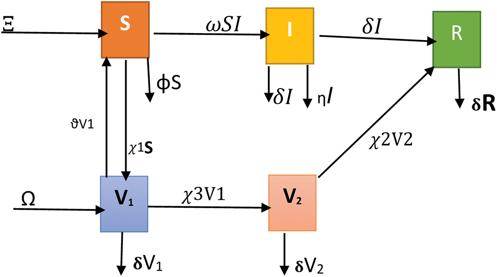
Figure 3: Flow chart for measles infection model
3.1 Qualitative Aspects of Measles Epidemic Model
Here, we will use the structural evaluation of deterministic dynamics to analyze the evolution of stochastic frameworks in this part. Additionally, the (23) solution pertains to the (24) mean. To get equilibria, we first investigate a measles epidemic model (23), and then we examine adequate requirements wherein the equilibria are locally stable.
Theorem 3.1. If there be a viable domain
Proof. Considering, the overall population in the system under discussion is provided by
After differentiation with respect to
Simple computations yield
It follows that
Assume that
Hence,
3.2 Disease-Free Equilibrium Point (DFEP)
In order to find the EP at which the outbreak is eliminated from the community is found in this section. Allowing the right hand sides of (23) to zero and
After simplification, we have
i.e., is the phase where no disease exists in the environment.
3.3 Stochastic Fundamental Reproductive Number
Here, the fundamental reproductive number for (24) can be evaluated by employing Itôs formula for twice differentiable mapping on
Now, by means of system (24), we have
It follows that
Higher order differentials
Taking into account the next-generation matrix, we computed
Hence, the stochastic fundamental reproductive number is
For the (24), we deliver an analogous stochastic eradication of transmission. In the long term, if
Theorem 3.2. If there be
Proof. By means of (23), we have
Performing integration from
It follows that
Assume that
In view of strong law, we have
arrives at
This leads to
If
At DFE, we have
This concludes that
3.5 Endemic Equilibrium Point (EEP)
Here, the equilibrium point at which the infection survives in the population is determined in this part. By putting all of the systems equations equal to zero, the EEP of model (23) can be determined as
After simplifying, then system (23) has the EEP as follows:
This section determines the importance of each component in the spread and prevention of measles infection through sensitivity evaluation. When a criterion improves, the investigation can help measure and compare the variation in a factor. This data is critical for studying the disease’s emergence and spread. With regard to a factor
The sensitivity values of the components of the measles illness framework are shown in the aforementioned evaluation. The following is a summary of sensitivity index comprehension.
The fundamental reproducing number’s responsiveness levels to the essential factors are addressed and presented in the previous analysis. As a result, the factors
4 A Fractional Stochastic Model of Measles Epidemic
Next, we investigate a generic measles stochastic model in which the standard temporal derivative is transformed into the global derivative in this part. It is specified as the GD of a differentiable mapping
In fact, if
Considering the system (24), we can simply evaluate the disease’s elimination and prevalence. For this, we assume the system (24) with respect to the global derivative as follows:
Since
It is important to mention that the framework is simple to determine if the ambient noise
Taking the integral on both sides, we have
In view of the Brownian motion, we have
With the classic GD, we obtain the complex stochastic equation below. Let us describe the requirement in which the nonlinear problem has a specific value, based on Atangana’s work [29,35].
Theorem 4.1. Assume there be positive constants
(a)
(b)
Proof. By means of model (29), we prove the Lipschitz condition for the proposed system as follows:
where,
Let us introducing the norm
then for all
where
where
Furthermore, we show that for all
where
Again, we show that for all
where
Now, we find for all
where
where
Now, we find for all
where
Next, in order to prove the linear growth conditions for model (29). To do this, for all
under supposition
Moreover,
under supposition
Furthermore, we have
under supposition
Again, we have
under supposition
Again, we have
under supposition
Now, we have
under supposition
Also, we have
under supposition
Clearly, we see that both assumptions are satisfied. Hence, according to the given hypothesis, the measles epidemic model (29) has a unique solution.
In what follows, the elimination of specific groups is discussed in this part. We did this by specifying
We shall begin using class
Multiplying both sides by
It follows that
Thus, we have
Considering the class
This leads to
Thus, we have
Analogously, we have
4.2 Numerical Scheme for Stochastic Model via Global Derivative
In this part, we use the Toufik et al. [36] technique to develop a numerical scheme for the stochastic framework (29) as follows:
Assuming that
Since
At
Again, at
Letting the difference of the two successive terms as follows:
Taking
Observe that
Furthermore, implementing the interpolation
Also, we have
Inserting the values of
and
5 Numerical Scheme for Fractional Stochastic Model via Global Derivative
The simulation tool for addressing the fractional order measles stochastic model involving GD is described in this section. We shall employ kernels of the exponential decay law and the M-L law to construct a highly meaningful approach. We shall employ Toufik et al. [36] numerical criteria to create the numerical results (29).
5.1 Caputo-Fabrizio Fractional Derivative Operator
First we demonstrate the numerical scheme for the Caputo-Fabrizio derivative operator:
Since
By making the use of Caputo-Fabrizio integral, we apply
Since
At
Further, at
For the sake of simplicity, we have
Furthermore, implementing the interpolation
Also, we have
Now, the interpolation polynomials are
It follows that
where,
After rearranging all expressions, we have
Now we can employ (43) technique on measles epidemics stochastic model:
and
5.2 Atangana-Baleanu Fractional Derivative Operator
Here, we illustrate the numerical scheme for the Atangana-Baleanu derivative operator:
Since
By making the use of Atangana-Baleanu integral, we apply
Since
At
For the sake of simplicity, we have
Furthermore, implementing the interpolation
Also, we have
Now, the interpolation polynomials are
Thus, we have
In view of the Lagrange interpolation polynomial technique, we have
After plugging the values of
Now we can employ (43) technique on measles epidemics stochastic model:
and
In what follows, we describe and investigate the system’s input variables, as well as simulation studies. We applied input variables from Table 1 further to simulate the constructed framework. The fractional stochastic mathematical formulation is expressed in the context of global derivative operators in terms of Caputo differential operators of visualizations developed with MATLAB via multiple fractional orders. This investigation is being carried out to determine the mechanisms of measles spreading in the community. Taking into account the technique of Toufik et al. [36], is utilized to determine the numerical configurations.

Figs. 4–6 demonstrate the stochastic behavior for different fractional orders in terms of global derivative in the Caputo-Fabrizio sense, demonstrating that the number of vulnerable, contaminated individuals diminishes from the beginning stage until a specific period
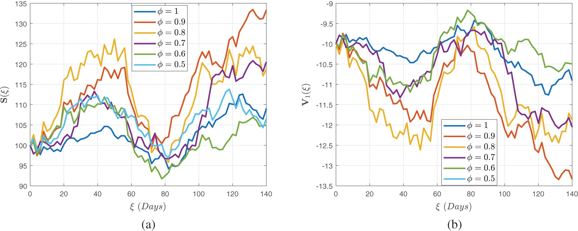
Figure 4: Stochastic behavior of the susceptible class
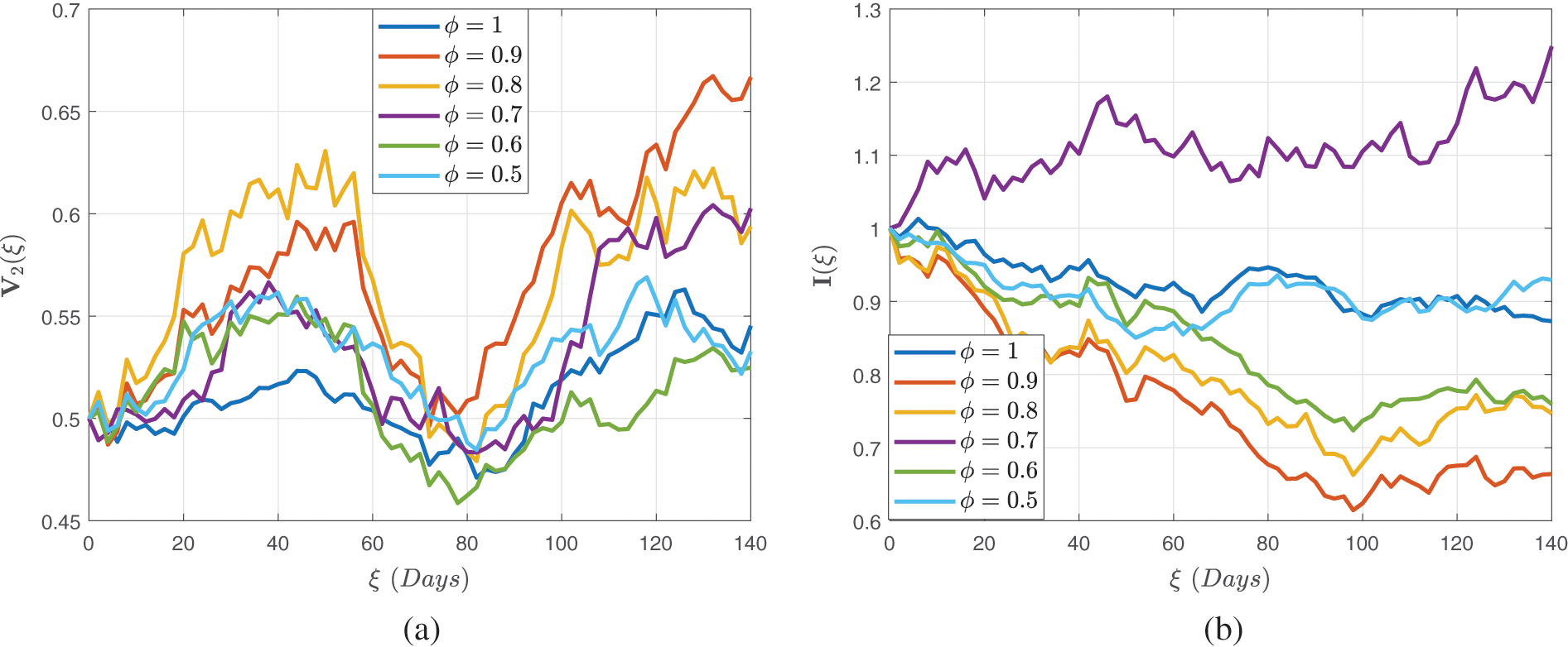
Figure 5: Stochastic behaviour of the dual dose vaccination group
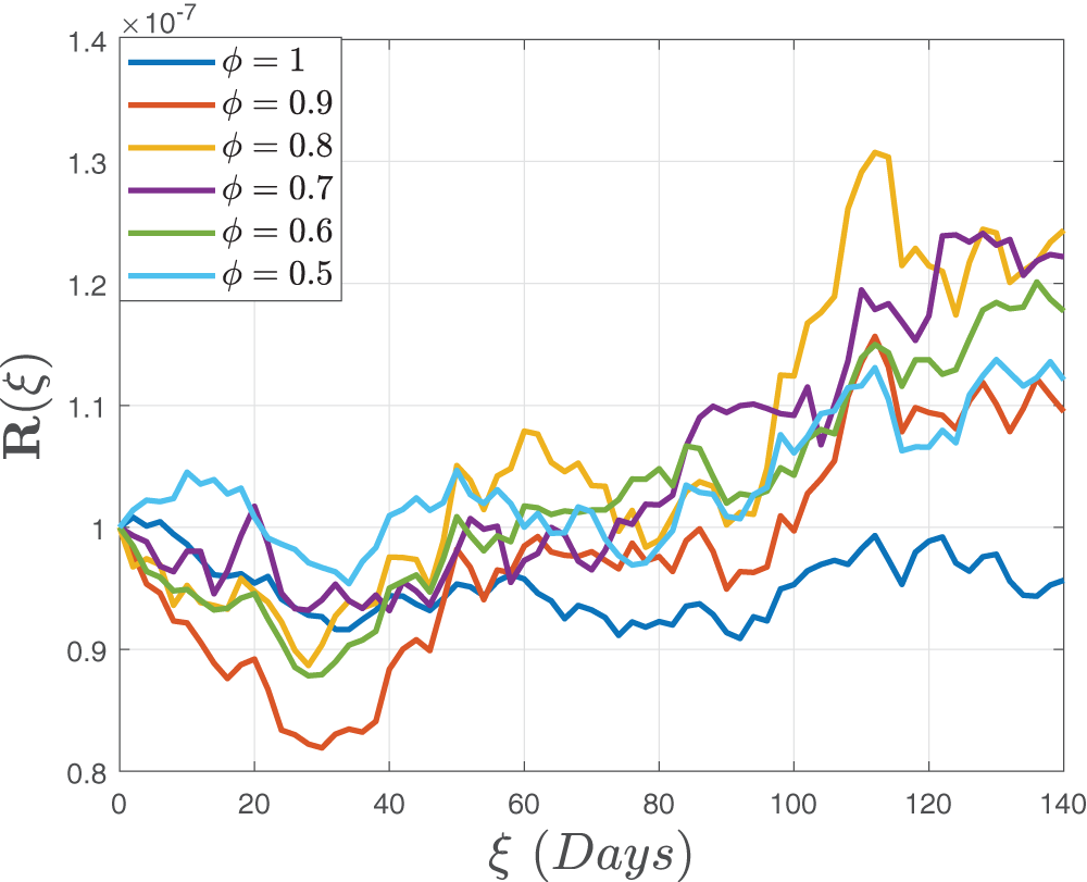
Figure 6: Stochastic behavior of the recovered class
In Figs. 7–9, we attempted to demonstrate how the interaction rate
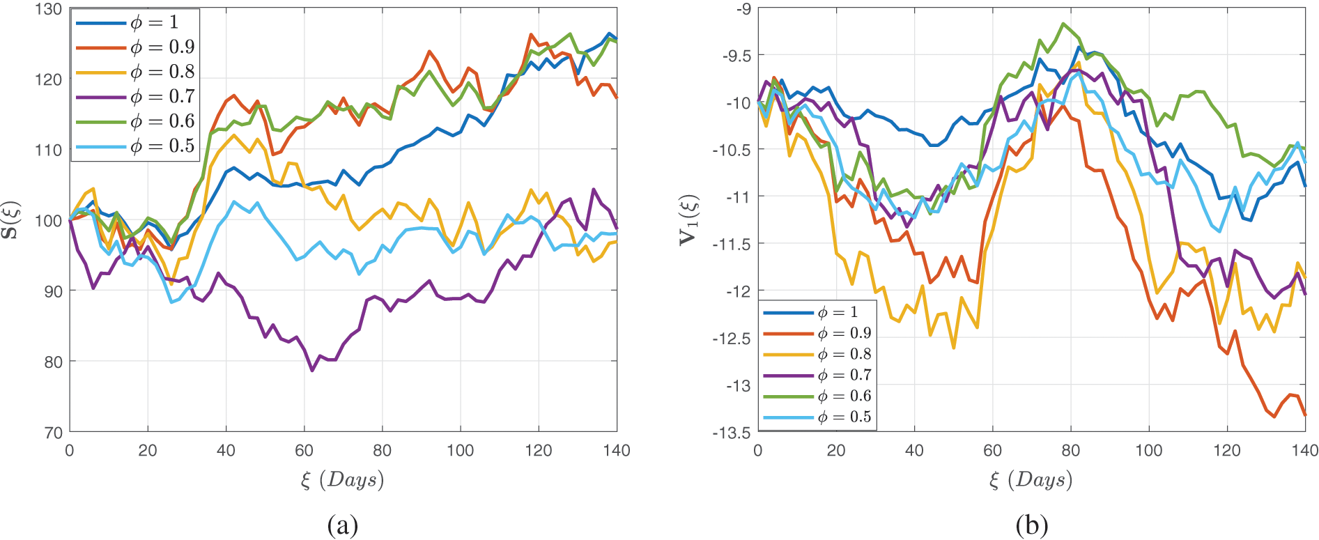
Figure 7: Stochastic behavior of the dual dose vaccination group
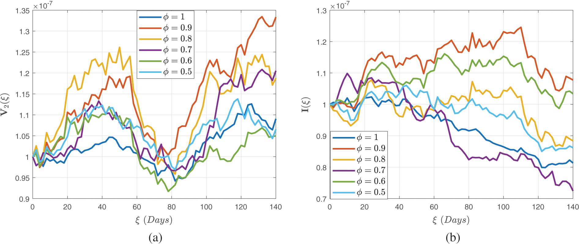
Figure 8: Stochastic behavior of the dual dose vaccination group
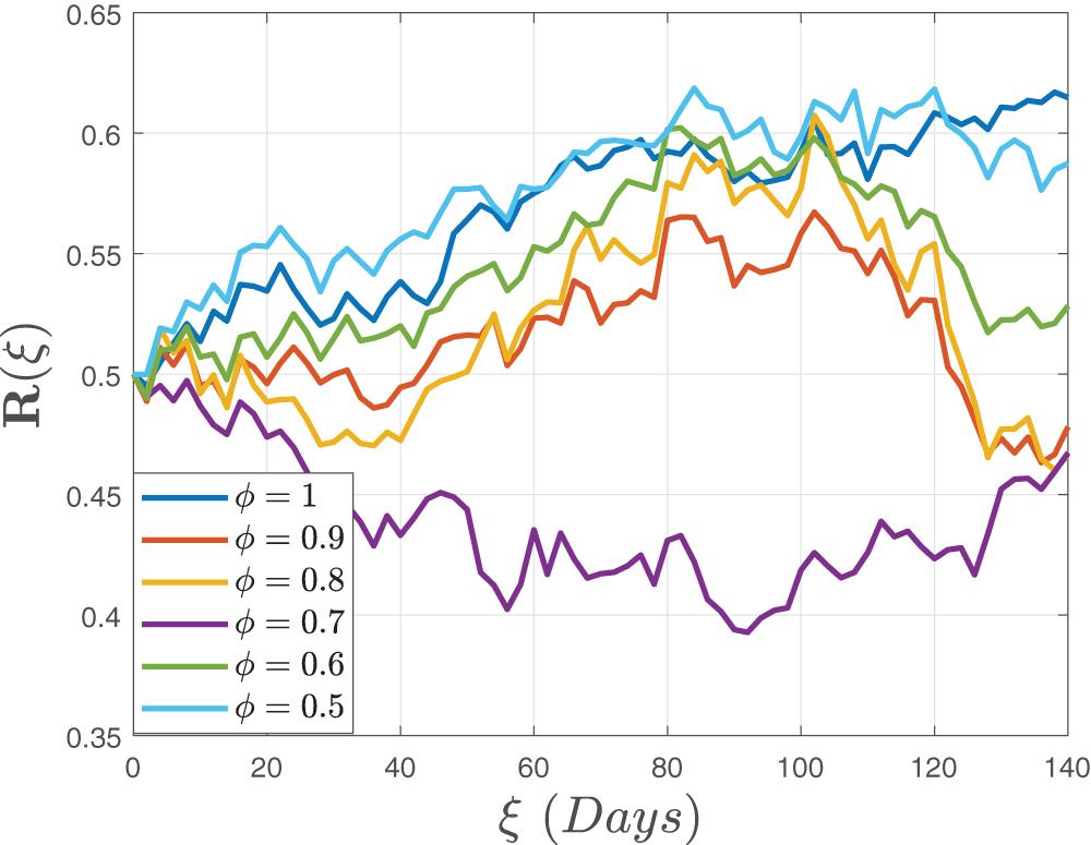
Figure 9: Stochastic behavior of the recovered class
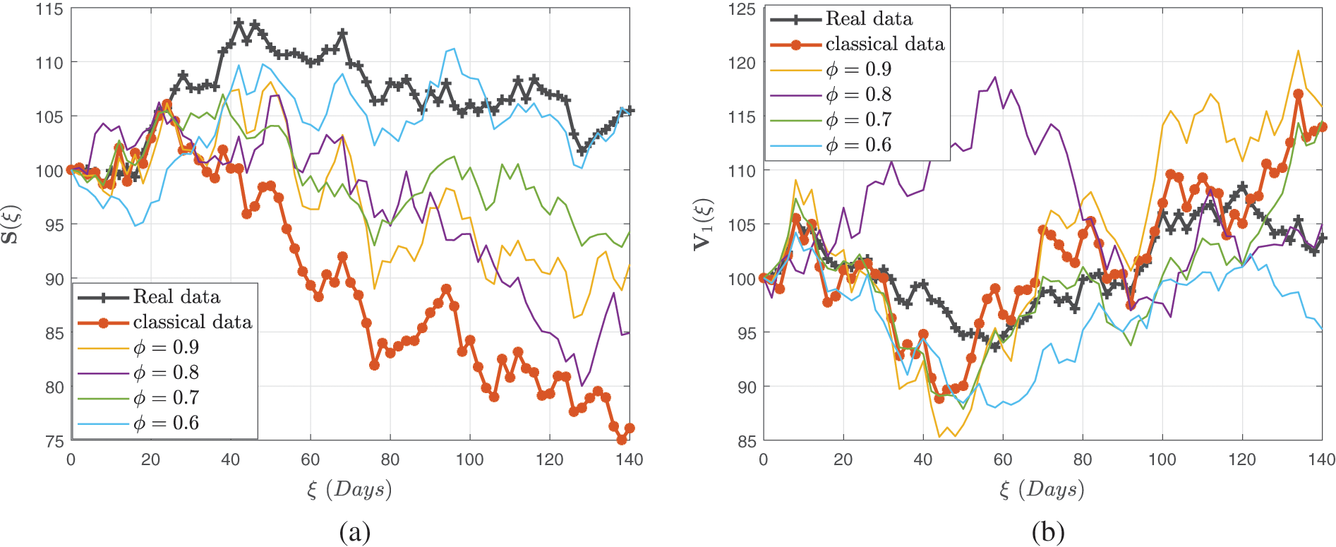
Figure 10: Stochastic behavior of the dual dose vaccination group
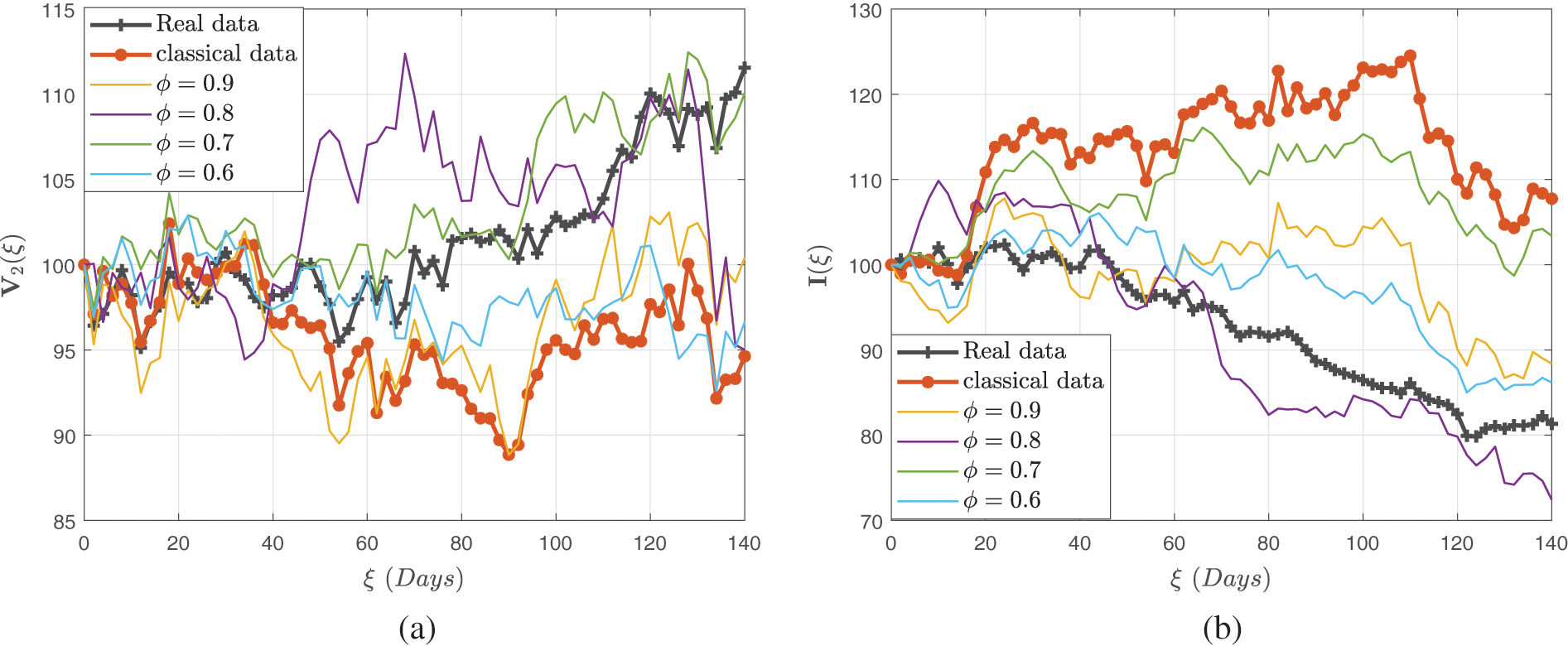
Figure 11: Stochastic behavior of the dual dose vaccination group

Figure 12: Stochastic behavior of the recovered class
This achievement was realized through meticulous verification of settings, which facilitated the observation of linear growth patterns and Lipschitz quadratic characteristics. With a numerical technique predicated on the Newton polynomial, each version was addressed differently. The influence of fractional-order and stochastic elements was demonstrated through modeling. Owing to the modeling studies via fractional operators, serious concerns like infection are not computationally intensive, so integrating fractional stochastic influences into the system makes modeling measles outbreaks considerably more authentic than the deterministic case. Our findings underscore the superior efficiency of a randomized model approach over a deterministic model in capturing the nuances of measles transmission dynamics, especially when considering dual-dose immunization strategies. As a result, we recommend using a stochastic approach to evaluate communicable disease trends; reducing interaction between vulnerable and infectious agent populations; increasing double-dose immunization penetration; and combining understanding and acceptance with therapy to eradicate measles in communities.
Acknowledgement: The researchers would like to thank the reviewers and editors for helping to improve this article.
Funding Statement: The authors received no specific funding for this study.
Author Contributions: The authors confirm their contribution to the paper as follows: study conception and design: S. Rashid and F. Jarad; data collection: S. Rashid; analysis and interpretation of results: S. Rashid and F. Jarad; draft manuscript preparation: S. Rashid and F. Jarad; software: F. Jarad; validation: S. Rashid. All authors reviewed the results and approved the final version of the manuscript.
Availability of Data and Materials: The datasets used and/or analyzed during the current study available from the corresponding author on reasonable request.
Conflicts of Interest: The authors declare that they have no conflicts of interest to report regarding the present study.
References
1. Moss, W. J., Griffin, D. E. (2012). Measles. Lancet, 379, 153–164. [Google Scholar] [PubMed]
2. CDC (Center of Disease Control) (2012). Progress in global measles control, 2000–2010. Morbidity and Mortality Weekly Report (MMWR), 61(4), 73–78. [Google Scholar]
3. Relief, D. (2012). The Global Measles Epidemic Isn’t (Just) about Measles. https://reliefweb.int/report/world/global-measles-epidemic-isn-t-just-about-measles (accessed on 21/04/2022). [Google Scholar]
4. Center of Disease Control and Prevention. Global Measles Outbreaks. https://www.cdc.gov/globalhealth/measles/data/global-measles-outbreaks.html (accessed on 12/06/2022). [Google Scholar]
5. Qureshi, S., Memon, Z. U. N. (2019). Monotonically decreasing behavior of measles epidemic well captured by Atangana-Baleanu-Caputo fractional operator under real measles data of Pakistan. Chaos Solitons Fractals, 131, 109478. [Google Scholar]
6. Qureshi, S., Atangana, A. (2020). Fractal-fractional differentiation for the modeling and mathematical analysis of nonlinear diarrhea transmission dynamics under the use of real data. Chaos, Solitons Fractals, 136, 109812. [Google Scholar]
7. Rihan, F. A., Baleanu, D., Lakshmanan, S., Rakkiyappan, R. (2014). On fractional SIRC model with Salmonella bacterial infection. Abstract and Applied Analysis, 2014, 136263. [Google Scholar]
8. Alkahtani, B. S. T., Alzaid, S. S. (2021). Stochastic mathematical model of Chikungunya spread with the global derivative. Results in Physics, 20, 103680. [Google Scholar]
9. Sans, W., Zhai, X., Sen, S., Collani, E. V. (2006). A note on nature and significance of stochastic models. Economic Quality Control, 21, 183–197. [Google Scholar]
10. Kermack, W. O., McKendrick, A. G. (1927). A contribution to the mathematical theory of epidemics. Proceedings of the Royal Society of London, 115, 700–721. [Google Scholar]
11. Atangana, A., Jain, S. (2018). A new numerical approximation of the fractal ordinary differential equation. The European Physical Journal Plus, 133, 37. https://doi.org/10.1140/epjp/i2018-11895-1 [Google Scholar] [CrossRef]
12. Atangana, A. (2017). Fractal-fractional differentiation and integration: Connecting fractal calculus and fractional calculus to predict complex system. Chaos Solitons Fractals, 102, 396–406. [Google Scholar]
13. Atangana, A., Rashid, S. (2022). Analysis of a deterministic-stochastic oncolytic M1 model involving immune response via crossover behaviour: Ergodic stationary distribution and extinction. AIMS Mathematics, 8, 3236–3268. [Google Scholar]
14. Atangana, A., Jain, S. (2019). Models of fluid flowing in non-conventional media: New numerical analysis. Discrete and Continuous Dynamical Systems Series S, 13(3), 467–484. https://doi.org/10.3934/dcdss.2020026 [Google Scholar] [CrossRef]
15. Lu, J. G. (2006). Chaotic dynamics of the fractional order Ikeda delay system and its synchronization. Chinese Physics, 15, 1–5. [Google Scholar]
16. Bhalekar, S. (2016). Stability and bifurcation analysis of a generalized scalar delay differential equation. Chaos, 26, 1–10. [Google Scholar]
17. Jain, S. (2018). Numerical analysis for the fractional diffusion and fractional Buckmaster’s equation by two-step Adam-Bashforth method. The European Physical Journal Plus, 133, 19. https://doi.org/10.1140/epjp/i2018-11854-x [Google Scholar] [CrossRef]
18. Iqbal, M. S., Yasin, M. W., Ahmed, N., Akgül, A., Rafiq, M. et al. (2023). Numerical simulations of nonlinear stochastic Newell-Whitehead-Segel equation and its measurable properties. Journal of Computational and Applied Mathematics, 418, 114618. [Google Scholar]
19. Attia, N., Akgül, A., Seba, D., Nour, A., Asad, J. (2022). A novel method for fractal-fractional differential equations. Alexandria Engineering Journal, 61, 9733–9748. [Google Scholar]
20. Bilal, S., Shah, I. A., Akgül, A., Tekin, M. T., Botmart, T. et al. (2022). A comprehensive mathematical structuring of magnetically effected Sutterby fluid flow immersed in dually stratified medium under boundary layer approximations over a linearly stretched surface. Alexandria Engineering Journal, 61, 11889–11898. [Google Scholar]
21. Saidu, A., Koyunbakan, H. (2022). Inverse fractional Sturm-Liouville problem with eigenparameter in the boundary conditions. Mathematical Methods in the Applied Sciences, 45, 11003–11012. [Google Scholar]
22. Rashid, S., Khalid, A., Sultana, S., Jarad, F., Abualnaja, K. M. et al. (2022). Novel numerical investigation of the fractional oncolytic effectiveness model with M1 virus via generalized fractional derivative with optimal criterion. Results in Physics, 37, 105553. [Google Scholar]
23. Christopher, O., Ibrahim, I. A., Shamaki, T. A. (2017). Mathematical model for the dynamics of Measles under the combined effect of vaccination and measles therapy. International Journal of Science and Technology, 31, 31–66. [Google Scholar]
24. Arqub, O. A., Okutachi, A. M. (2017). Simulating deterministic and stochastic differential equation models of measles outbreak considering population size and initial vaccination regime. Journal of Scientific and Engineering Research, 4, 271–282. [Google Scholar]
25. Edward, S., Raymond, K. E., Gabriel, K. T., Nestory, F., Godfrey, M. G. et al. (2015). A mathematical model for control and elimination of the transmission dynamics of measles. Applied and Computational Mathematics, 4, 396–408. [Google Scholar]
26. Podlubny, I. (1999). Fractional differential equations. New York: Academic Press. [Google Scholar]
27. Caputo, M., Fabrizio, M. (2015). A new definition of fractional derivative without singular kernel. Progress in Fractional Differentiation and Applications, 1, 73–85. [Google Scholar]
28. Atangana, A., Baleanu, D. (2016). New fractional derivatives with non-local and non-singular kernel. Theory and application to heat transfer model. Thermal Science, 20, 763–769. [Google Scholar]
29. Atangana, A. (2020). Extension of rate of change concept: From local to nonlocal operators with applications. Results in Physics, 19, 103515. [Google Scholar]
30. Tornatore, E., Buccellato, S. M., Vetro, P. (2005). Stability of a stochastic SIR system. Physica A: Statistical Mechanics and its Applications, 354, 111–126. [Google Scholar]
31. Iannelli, M. (1985). Mathematical problems in the description of age structured populations. In: Capasso, V., Grosso, E., Paveri-Fontana, S. L. (Eds.). Mathematics in biology and medicine, pp. 19–32. Berlin, Heidelberg: Springer. https://doi.org/10.1007/978-3-642-93287-8_3. [Google Scholar] [CrossRef]
32. Anderson, R. M., May, R. M. (1979). Population biology of infectious diseases, part I. Nature, 280, 361–367. [Google Scholar] [PubMed]
33. Gray, A., Greenhalgh, D., Hu, L., Mao, X., Pan, J. (2011). A stochastic differential equation SIS epidemic model. SIAM Journal on Applied Mathematics, 71, 876–902. [Google Scholar]
34. Mao, X. (1997). Stochastic differential equations and applications. Horwood Publishing Chichester. [Google Scholar]
35. Atangana, A. (2020). Modelling the spread of COVID-19 with new fractal-fractional operators: Can the lockdown save mankind before vaccination? Chaos Solitons Fractals, 136, 109860. [Google Scholar] [PubMed]
36. Toufik, M., Atangana, A. (2017). New numerical approximation of fractional derivative with non-local and non-singular kernel: Application to chaotic models. The European Physical Journal Plus, 132, 444. [Google Scholar]
37. Raymond, K. (2016). Stochastic modeling of the transmission dynamics of measles with vaccination control. International Journal of Theoretical and Applied Methematics, 2, 60–73. [Google Scholar]
Cite This Article
 Copyright © 2024 The Author(s). Published by Tech Science Press.
This work is licensed under a Creative Commons Attribution 4.0 International License , which permits unrestricted use, distribution, and reproduction in any medium, provided the original work is properly cited.
 Downloads
 Citation Tools