
 Submit a Paper
 Propose a Special lssue
 Open Access
ARTICLE

Novelty of Different Distance Approach for Multi-Criteria Decision-Making Challenges Using q-Rung Vague Sets
1 Saveetha School of Engineering, Saveetha Institute of Medical and Technical Sciences, Chennai, 602105, India
2 Department of Mathematics, Faculty of Arts and Science, Yildiz Technical University, Esenler, Istanbul, 34220, Turkey
3 Department of Operations Research and Statistics, Faculty of Organizational Sciences, University of Belgrade, Belgrade, 11000, Serbia
4 College of Engineering, Yuan Ze University, Taoyuan City, 320315, Taiwan
5 Department of Applied Data Science, Noroff University College, Kristiansand, 4612, Norway
6 Artificial Intelligence Research Center (AIRC), Ajman University, Ajman, 346, United Arab Emirates
7 Department of Electrical and Computer Engineering, Lebanese American University, Byblos, 1102-2801, Lebanon
8 ICT Convergence Research Center, Soonchunhyang University, Asan, 31538, South Korea
9 Department of Computer Science and Engineering, Soonchunhyang University, Asan, 31538, South Korea
* Corresponding Authors: Nasreen Kausar. Email: ; Seifedine Kadry. Email:
(This article belongs to the Special Issue: Advances in Ambient Intelligence and Social Computing under uncertainty and indeterminacy: From Theory to Applications)
Computer Modeling in Engineering & Sciences 2024, 139(3), 3353-3385. https://doi.org/10.32604/cmes.2024.031439
Received 16 June 2023; Accepted 06 September 2023; Issue published 11 March 2024
 View Full Text
 Download PDF
Abstract
In this article, multiple attribute decision-making problems are solved using the vague normal set (VNS). It is possible to generalize the vague set (VS) and q-rung fuzzy set (FS) into the q-rung vague set (VS). A log q-rung normal vague weighted averaging (log q-rung NVWA), a log q-rung normal vague weighted geometric (log q-rung NVWG), a log generalized q-rung normal vague weighted averaging (log Gq-rung NVWA), and a log generalized q-rung normal vague weighted geometric (log Gq-rung NVWG) operator are discussed in this article. A description is provided of the scoring function, accuracy function and operational laws of the log q-rung VS. The algorithms underlying these functions are also described. A numerical example is provided to extend the Euclidean distance and the Humming distance. Additionally, idempotency, boundedness, commutativity, and monotonicity of the log q-rung VS are examined as they facilitate recognizing the optimal alternative more quickly and help clarify conceptualization. We chose five anemia patients with four types of symptoms including seizures, emotional shock or hysteria, brain cause, and high fever, who had either retrograde amnesia, anterograde amnesia, transient global amnesia, post-traumatic amnesia, or infantile amnesia. Natural numbers q are used to express the results of the models. To demonstrate the effectiveness and accuracy of the models we are investigating, we compare several existing models with those that have been developed.Keywords
Abbreviations
| DM | Decision-making |
| MADM | Multiple-attribute decision-making |
| MCDM | Multi-criteria decision-making |
| TOPSIS | Technique for order of preference by similarity to ideal solution |
| FS | Fuzzy set |
| IFS | Intuitionistic fuzzy set |
| PyFS | Pythagorean fuzzy set |
| PyIVFS | Pythagorean interval-valued fuzzy set |
| NSS | Neutrosophic set |
| SFS | Spherical fuzzy set |
| VS | Vague set |
| TMG | Truth membership grade |
| IMG | Indeterminacy membership grade |
| FMG | False membership grade |
| ED | Euclidean distance |
| HD | Hamming distance |
| AO | Aggregating operator |
| q-ROFS | q-rung orthogonal pair fuzzy set |
| q-ROFWABM | q-rung orthopair fuzzy weighted Archimedean Bonferroni mean |
| q-ROFABM | q-rung orthopair fuzzy Archimedean Bonferroni mean |
| q-ROFPA | q-rung orthopair fuzzy power averaging |
| q-ROFPWA | q-rung orthopair fuzzy power weighted average |
| q-ROFPWMSM | q-rung orthopair fuzzy power weighted Maclaurin symmetric mean |
| q-ROFWA | q-rung orthopair fuzzy weighted average |
| q-ROFWG | q-rung orthopair fuzzy weighted geometric |
| log q-rung VNN | log q-rung vague normal number |
| log q-rung NVWA | log q-rung normal vague weighted average |
| log q-rung NVWG | log q-rung normal vague weighted geometric |
| log G q-rung NVWA | log generalized q-rung normal vague weighted average |
| log G q-rung NVWG | log generalized q-rung normal vague weighted geometric |
Decision-makers find it increasingly difficult to identify the optimal solution as real-world systems become increasingly complex. Selecting the best option is possible difficulty of deciding between the alternatives. Opportunities, objectives, and viewpoint constraints are challenging to create for many firms. In line with this, when decisions making (DM), individuals or groups should consider multiple objectives at the same time. A wide variety of MADM-related issues are dealt with every day. Our DM abilities need to be improved as a result. This field of study has been studied by a variety of researchers using a variety of methods. There are several uncertain theories proposed by them to deal with the uncertainties, including fuzzy set (FS) [1], intuitionistic fuzzy set (IFS) [2], interval valued FS (IVFS) [3], vague set [4], Pythagorean fuzzy set (PFS) [5], IVPFS [6], spherical FS (SFS) [7]. A membership grade (MG) indicates how well an FS fits into the specified set with ranging from 0 to one. An IFS was defined by Atanassov [2] as having a total of membership grade (MG) and non-membership grade (NMG) less than one. The sum of the MG and NMG is sometimes greater than one when a DM method is applied. Yager [5] developed PFS, which is characterized by a square sum of its MG and NMG not exceeding one. In order to generalize IFS, Yager used PFS to build a model. A new concept has been proposed by Yager [8] in light of society’s continuous complexity and theory development. The MG and NMG in the q-rung orthogonal pair FS (q-ROFS) have power q, but the sum can never exceed one. The IFSs and PFSs can all be considered special cases of q-ROFSs, therefore they are general. There are more orthopairs that meet the bounding constraint as rung q increases, and as rung q increases, the space of acceptable orthopairs increases. The use of q-ROFSs can thus express fuzzy information in a broader range. Because the parameter q can be adjusted, q-ROFSs are flexible and better suited to uncertain environments. An increase in q can be made as ambiguity in decision information increases. It is possible that some experts are influenced by both their own desires and their surroundings. Therefore, they may have an MDG of 0.95 and an NMG of 0.55 when evaluating certain decision-making things. The fuzzy information cannot be described by IFNs and PFNs, but q-ROFNs can be described if parameter q is increased. Due to this, the q-ROFS is more flexible and suitable for describing uncertain data.
A discussion of the q-Rung Orthopair fuzzy weighted Archimedean Bonferroni mean (q-ROFWABM) and q-Rung Orthopair fuzzy Archimedean Bonferroni mean (q-ROFABM) operators was given in Liu et al. [9]. Liu et al. [10] proposed a concept of q-rung orthopair fuzzy power averaging (q-ROFPA), q-rung orthopair fuzzy power weighted average (q-ROFPWA), q-ROFPMSM and q-rung orthopair fuzzy power weighted MSM (q-ROFPWMSM) operators for q-ROFNs, describing their properties. Liu et al. [11] discussed the q-rung orthopair fuzzy weighted average (q-ROFWA) and q-rung orthopair fuzzy weighted geometric (q-ROFWG) operators are introduced and their basic properties are discussed. The concept of an incomplete probabilistic linguistic preference relation (InPLPR) was introduced by Wang et al. [12]. In 2013, Liu et al. [13] presented the concept of unit cost consensus adjustment based on a group consensus decision model based on InPLPR that takes into account social trust networks, consistency, and social trust networks. In a recent study, Zhang et al. [14] discussed three types of multi-granularity q-rung orthopair fuzzy preference relations (PRS) as well as their interesting properties. With the MAGDM algorithm based on q-ROF multi-attribute rules, the MG-3WD approach can also be applied to q-ROF complex information systems. Zhang et al. [15] analyzed a UCI dataset using MGq-ROF PRSs, the MULTIMOORA method, and the TPOP method using the MAGDM method. Zhang et al. [16] discussed neutosophic fusion of RST based on basic models and soft sets models. Based on fuzzy granularity spaces with properties that correspond to fuzzy knowledge distances, Lian et al. [17] discussed fuzzy relative knowledge distances. Furthermore, it has been demonstrated that fuzzy knowledge distances contain different structure information than precise knowledge distances. The hybridization of archimedean copulas and generalized MSM operators, based on q-rung probabilistic dual hesitant fuzzy sets, was discussed by Anusha et al. [18]. Multi-attribute decision-making (MADM) [19,20] offers an efficient means of evaluating multiple alternatives based on their evaluation values. Usually, MADM problems can be solved in one of two ways. Traditional approaches, such as TOPSIS, VIKOR, ELECTRE, are examples. Information integration problems are more effectively solved by AOs than by traditional approaches. In contrast to traditional approaches, AOs provide comprehensive values of all alternatives, rather than ranking results only. In his article, Bairagi [21] used extended TOPSIS to select homogeneous groups of robotic systems.
This is insufficient for demonstrating neutrality (neither favor nor disfavor). It was developed by Cuong et al. [22] with a total grade no higher than one for three pointers such as positive, neutral, and negative. As a result, it would be appropriate for the DM method to use this set over IFS or PFS for selective applications. Liu et al. first presented the concept of an aggregation operator (AO) in generalized PFS [23]. A PIVFS algorithm for the problem of identifying truth membership grades (TMGs), indeterminacy membership grades (IMGs) and false membership grades (FMGs) with AOs [6,24–26] have the feature that the sum of the three grades (TMG, IMG, and FMG) is greater than one. It has been suggested by Ashraf et al. [7] that the SFS should contain the following graph: this diagram shows that the sum of the squares of the TMG, IMG and FMG should be not exceeds one. To analyze the idea of SFS, Fatmaa et al. [27] used the TOPSIS technique as part of their study. There have been several different concepts of q-Rung picture FS with AO for DM that have been demonstrated by Liu et al. [28]. In addition to Biswas [4], there is a concept of VSs VS is called to the two functions TMG
As an alternative to algebraic operations, a log q-rung arithmetic operation can provide a smooth estimate quality that is similar to that of a continuous algebraic operation when compared with its smoothness. Compared to the log q-rung arithmetic operations on the IFS and PFS only a limited research has been done on log q-rung arithmetic operations. Our method of VS is based on log q-rung arithmetic AOs within VSs rather than using log q-rung arithmetic operations. The use of spherical fuzzy q-rung arithmetic AOs based on entropy in DM, as well as their real-life application to the problem, were introduced by Jin et al. [40]. Ashraf et al. [41] proposed by that linear-logarithmic hybrid AOs be used for single-valued neutrosophic sets. Palanikumar et al. have examined the new type Pythagorean fuzzy set with AO [42]. Yager [5] has also presented an average and geometric AO using PFS weighted and weighted power cases. A number of basic PFS features were discussed by Peng et al. [43]. A generalized PFS under AO has been developed by Liu et al. [23]. Adak et al. dicussed the concept of spherical distance measurement method for solving MCDM problems under PFS [44]. Some picture fuzzy mean operators and their applications in DM is discussed by Hasan et al. [45]. Mishra et al. [46] discussed the new concept of Pythagorean and Fermatean fuzzy sub-group redefined in context of T-norm and S-conorm. DM analysis of minimizing the death rate due to COVID-19 by using q-rung orthopair fuzzy soft bonferroni mean operator discussed by Abbas et al. [47]. Yaman et al. [48] discussed the new approach for warehouse location decisions changed in medical sector after pandemic study. Recently, FS and its extension including q-rung orthopair fuzzy set, T-spherical fuzzy set based on decision making approach [49–55]. The log q-rung information about the VNS was obtained utilizing OAs. Section 2 explains the given information about the FS and VS components. Section 3 explains the definition of q-rung vague sets as well as the different operations involved with them. There is a discussion on ED and HD in Section 4 using the log q-rung vague normal number (log q-rung VNN). A MADM connection is established through the Section 5 using log q-rung VNNs. Section 6 contains a numerical example and a description of log q-rung VS as well as the insert algorithm and log q-rung VS application. We provide a conclusion in Section 7. An overview of the key things that were taken into account during the research process is given below:
1. As a result of log-rung VNSs, ED and HD were introduced.
2. The log q-rung VNVWA, log q-rung VNVWG, log Gq-rung VNVWA, and log Gq-rung VNVWG operators were suggestions.
3. A log-rung VNS is used in order to explore the MADM technique.
4. We evaluate log q-rung VNVWA, log q-rung VNVWG, log Gq-rung VNVWA and log Gq-rung VNVWG in order to establish optimal value parameters.
5. An analysis of the proposed and early investigations is presented along with a comparative analysis.
6. DM outcomes for natural numbers with a value of q.
We will introduce some basic literature on Pythagorean fuzzy set, Pythagorean interval-valued fuzzy set, vague set and spherical fuzzy set in the section, which will be useful in later section. Additionally, the basic operating rules and zero vague and unit vague set of these concepts are discussed.
Definition 2.1. [5] Let U be the universal, PFS M in U is
Definition 2.2. [6] The PIVFS M in U is
For
Definition 2.3. [4] (i) A VS M in U is a pair
(ii)
Definition 2.4. [4] (i) A VS M is contained in VS
(ii) Union of M and
(iii) Intersection of M and
Definition 2.5. [4] A VS M of
(i)
(ii)
Definition 2.6. [38] The fuzzy number
Definition 2.7. [39] Let
3 log q-rung NVN and Its Basic Operations
In this section, we develop some novel logarithmic operational laws for normal vague numbers and discuss their properties. The main purpose of this section is to propose novel logarithmic aggregation operators based on normal vague information. The logarithmic function offers versatility in supporting the decision experts choices during object appraisal due to its periodic and symmetric character. An important fundamental operation of the log q-rung normal number is defined.
Definition 3.1. The log VS M in U is
Definition 3.2. Let
Definition 3.3. Let
The score function of M is
The accuracy function of M is
where
Definition 3.4. Let
1.
2.
3.
4.
4 Distance between log q-rung Normal Vague Numbers
The Euclidean distance and Hamming distance are useful technique for calculating the distance between two elements, two sets, etc. In order to define the Euclidean distance and Hamming distance, first, we will define a distance measure. Basically, a distance measure has to accomplish the following properties. This study examined the mathematical properties of log q-rung NVNs and measured the expectation of ED and HD.
Definition 4.1. Let
and HD between
Theorem 4.1. Let
1.
2.
3.
Corollary 4.1. Let
1.
2.
3.
5 log q-rung Normal Vague Number Using AOs
We will introduce the novel concepts of log q-rung NVWA, log q-rung NVWG, log G q-rung NVWA, and log G q-rung NVWG operators utilizing log q-rung NVN.
Definition 5.1. Let
Theorem 5.1. Let
Theorem 5.2. (idempotency property) If all
Theorem 5.3. (boundedness property) Let
Then,
where
Theorem 5.4. (monotonicity property) Let
Definition 5.2. Let
Theorem 5.5. Let
Theorem 5.6. If all
Corollary 5.1. Boundness and monotonicity properties can be satisfied using the log q-rung NVWG operator.
5.3 log G q-rung NVWA Operator
Definition 5.3. Let
Theorem 5.7. Let
Theorem 5.8. If all
Corollary 5.2. By using log G q-rung NVWA operators, it is possible to satisfy bounding and monotonicity properties.
5.4 log G q-rung NVWG Operator
Definition 5.4. Let
Theorem 5.9. Let
The log G q-rung NVWG operations are modified to be log q-rung NVWG operations with q = 1.
Corollary 5.3. The log G q-rung NVWG operator is able to satisfy properties such as boundness and monotonicity.
Corollary 5.4. If all
6 log q-rung NVN Based on MADM
Let
Let
Since
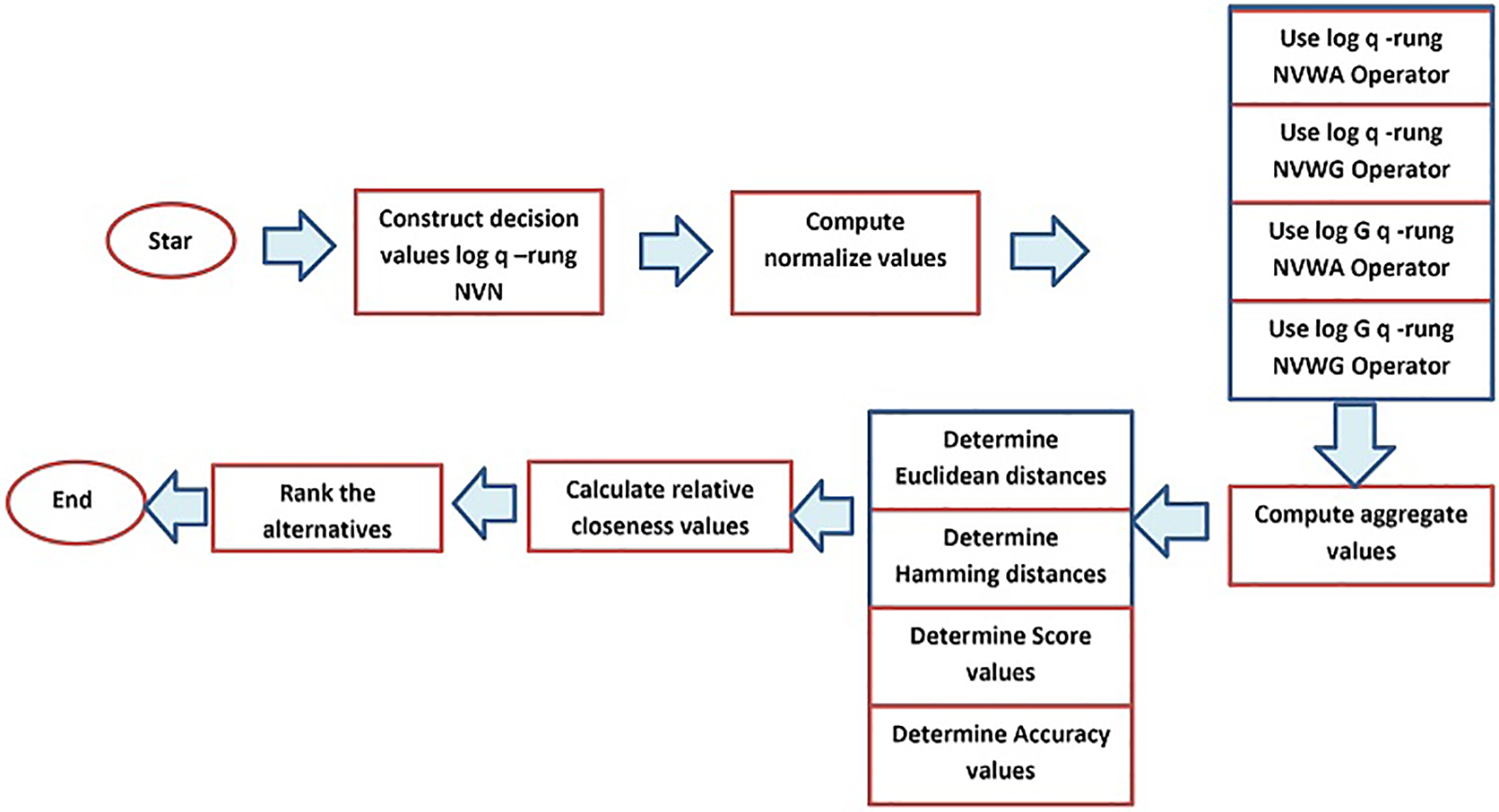
Figure 1: Flowchart of the MADM algorithm
Step-1: The log q-rung NVN values that can be input.
Step-2: Calculate the normalized values for the DM. The decision matrix n × m as
Step-3: By utilizing log q-rung NVN, you can determine the aggregate values for all alternative based on AOs, attribute
Step-4: Calculate the positive and negative ideal values for each case as follows:
Step-5: Determine the EDs between the alternatives with a positive and a negative ideal value so as to determine the value of each alternative as
Step-6: It is possible to calculate the relative closeness values by using the following formula:
Step-7: The optimal value is
6.2 Selection of Amnesia Patients
A person with anemia has insufficient or malfunctioning red blood cells. A man is diagnosed with anemia when his hemoglobin value is below 13.5 gm/dl, while a woman is diagnosed with anemia when her hemoglobin value is below 12.0 gm/dl. There are a variety of normal values for children depending on their age. Memory strategies are used to help deal with amnesia. Taking care of underlying diseases that cause amnesia is also important. An occupational therapist may help the person learn new information and replace what they have lost. Taking in new information may be based on intact memories. Additionally, memory training can help organize information to make it easier to remember and to better understand when you are speaking with others. Smartphones and hand held tablets are often used by people with amnesia. A simple electronic organizer can help even people who suffer from severe amnesia stay on top of their daily activities with a little training and practice. A person with amnesia may benefit from psychological therapy or cognitive behavioral therapy (CBT). When it comes to recalling forgotten memories, hypnosis can be very effective. It is important to retrieve memories and deal with psychological issues that may have contributed to amnesia as part of treatment for amnesia. A person may be able to retrieve forgotten memories through meditation and related mindfulness activities. It is also imperative to have your family's support. Playing familiar music, showing them photographs from the past, and exposing them to familiar scents may be helpful. Blood buildup in the brain may cause amnesia in people who have been injured in head trauma. Anti-inflammatory medications may be needed by people with encephalitis. If you cycle, skate, ski, or play contact sports, you may be at greater risk of developing amnesia due to headgear. It is important to consume a diet rich in leafy green vegetables and avoid saturated fats to prevent cardiovascular diseases that can negatively affect memory. Brain regulation is achieved through the Bilateral Sounds method. As well as relieving stress and symptoms of PCS and PTSD, it is excellent for reeducating the left and right hemispheres. There are some commonly used bilateral sounds available for this purpose through Psych Innovations, a web-based company.
1. Retrograde amnesia (A):A person suffering from retrograde amnesia is incapable of recalling past events. Memory loss usually affects memories made recently, not ones from years ago. You can experience amnesia if you lose the ability to make, store, and retrieve memories. Memory formation prior to amnesia onset is affected by retrograde amnesia. After a traumatic brain injury, a person may develop retrograde amnesia, which prevents him or her from remembering what happened decades earlier. A variety of brain regions can be damaged, causing retrograde amnesia to occur.
2. Anterograde amnesia (B):The type of amnesia that causes this is when you forget anything that has happened since your amnesia began. Even if you have a state of amnesia, you can still recall information you recall before the amnesia occurred. Unlike retrograde amnesia, this occurs more frequently. During an amnesia-inducing event, there is no memory creation after anterograde amnesia occurs. It is possible to suffer from anterograde amnesia either to the extent of being unable to remember events only partially or completely. In this case, a person with amnesia has retained long-term memories from the time before the incident occurred. In anterograde amnesia, new memories cannot be encoded (or possibly retrieved). As well as different severity levels of anterograde amnesia, some individuals forget recent events such as meals or phone numbers, while others forget what they were doing a few seconds ago. Memory is also affected by the difficulty of a task, with more complex tasks being harder to remember than simpler tasks that do not require as much mental energy.
3. Transient global amnesia (TGA) (C):It tends to resolve within 24 h if it is a temporary amnesia. Adults over the age of middle age and those who are older are more likely to experience it. It is rare for such amnesia to recur once it has resolved. Someone who is otherwise alert may experience transient global amnesia, which manifests itself suddenly as confusion. A person with transient global amnesia cannot create new memories, so the memory of recent events is lost. This condition is not caused by something more common, such as epilepsy or stroke. Neither you nor how you got here can be recalled. What’s going on right now may not be clear to you. The answers you have just been given may not stick in your memory, so you keep repeating the same questions. Similarly, it is possible to lose track of events from a month ago if you are asked to recall them. People in their middle and older years are most likely to suffer from this condition. Transient global amnesia also leaves you recognizing people you know and remembering who you are. There are always a few hours of recovery time after an episode of transient global amnesia. Your memory may begin to return during recovery. It is not dangerous, but transient global amnesia can still be frightening.
4. Post-traumatic (D):Amnesia can occur either anterogradely or retrogradely after an injury to the head. Post-traumatic amnesia is a type of memory loss that occurs immediately after a traumatic brain injury (TBI). This state is characterized by disorientation and inability to remember past events. An individual may be incapable of stating their name, location, and time. It is considered that PTA has been resolved when continuous memory returns. The memory is not able to store new events during PTA. The memory of some incidents is only recalled by one third of patients with mild head injuries. There is a “clouding” of consciousness experienced by the patient during PTA. It has been proposed as an alternative term for PTA since it includes confusion along with the memory loss typically associated with amnesia.
5. Infantile amnesia (E):Children often have difficulty recalling early childhood memories, which is referred to as childhood amnesia. The brains of young children are still developing, so they are incapable of consolidating memories. The ailment of being unable to recall episodic memories in adults younger than two to four years of age is known as childhood amnesia. During these years, the recollection of early childhood memories may also be scarce or fragmented, especially if they occurred between the ages of 2 and 6. Others believe that early memories are encoded and stored differently when a cognitive self is developed. The onset of childhood amnesia has differed between psychologists, but some research shows that children can recall things before they are two years old. As children grow, their memories may decline. An individual can recall their first memory at a certain age, according to some definitions. As a general rule, it occurs at the age of two to four, but this can vary from child to child.
The four factors are
1. Seizures (
2. Emotional shock or hysteria (
3. Brain cause (
4. High fever (
Suppose that five anemia patients as
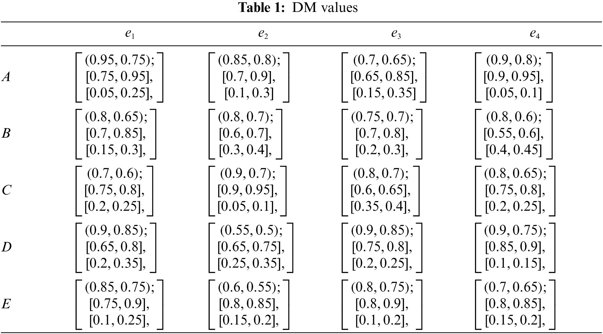
Step 1: Table 1 represents the DM values.
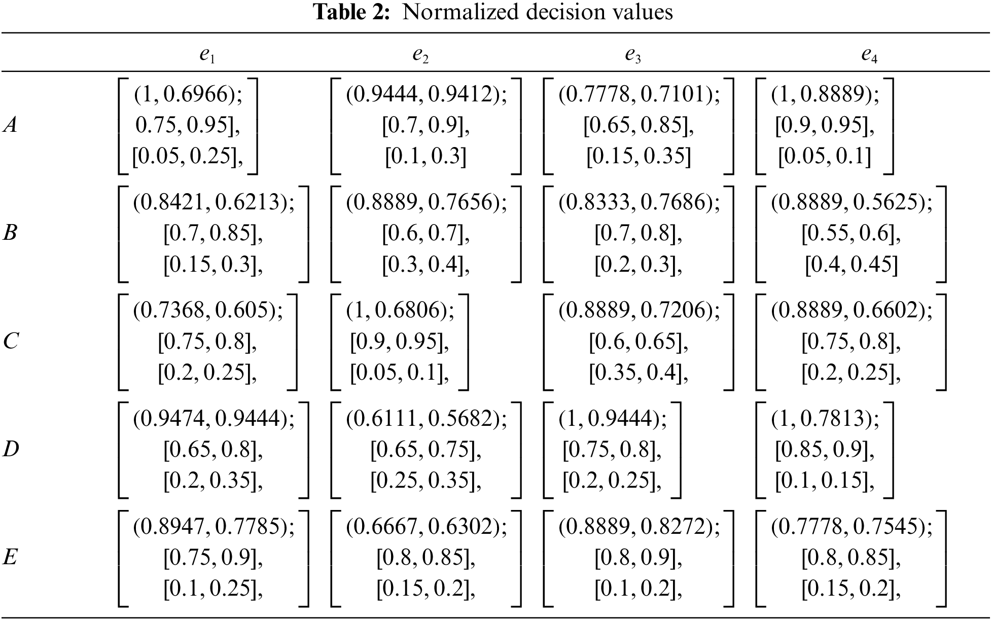
Step 2: Obtain normalized decision matrix: Table 2 represents the normalized decision values.
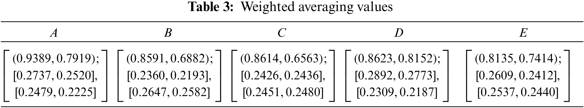
Step 3: For every alternative (q = 1), the aggregated information will be derived using log q-rung NVWA operators. Table 3 represents the weighted averaging values.
Step 4: Both of the ideal values for all alternative are as follows:
and
Step 5: The HD between for all alternative with a different ideal value is as follows:
and
Step 6: Relative closeness values are
Step 7: Ranking of alternatives are
Therefore A is a very urgent need for treatment.
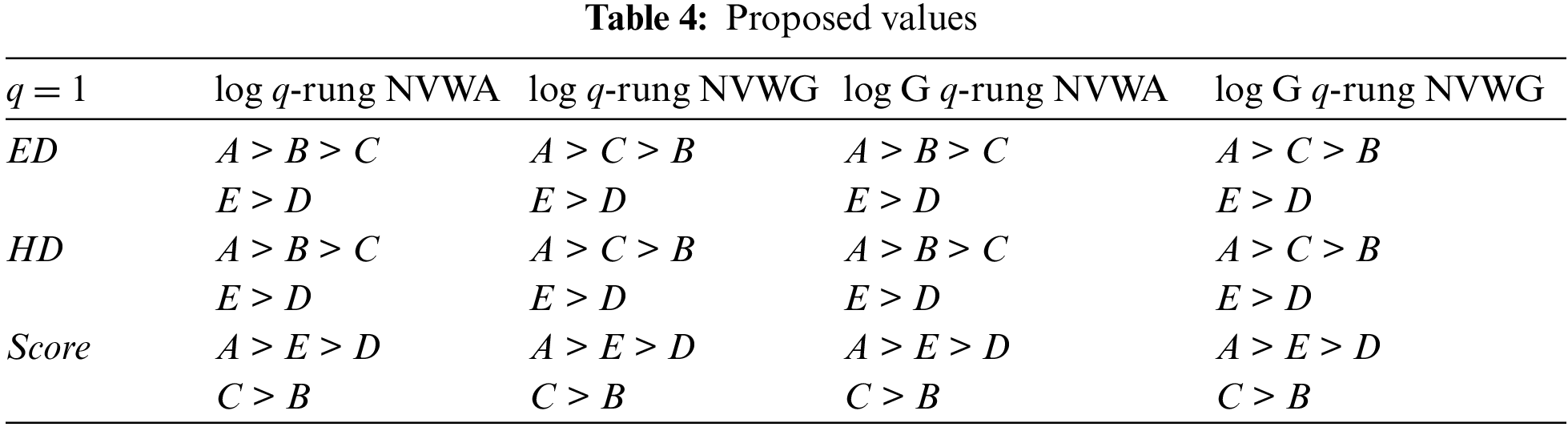
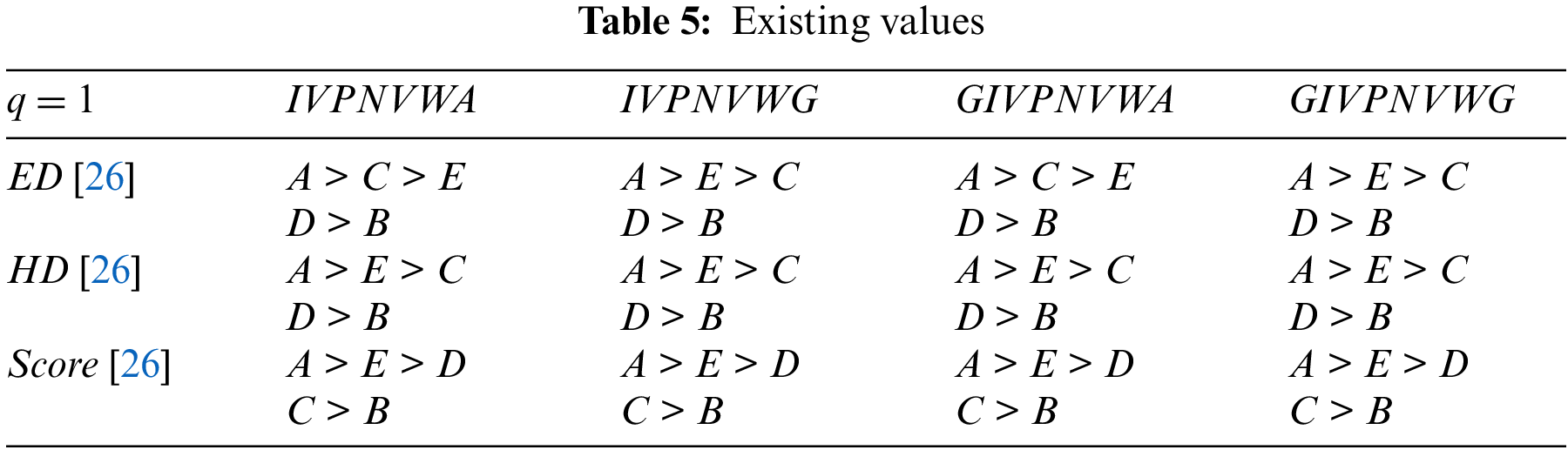
6.3 Comparison of the Suggested Method with Existing Methods
Here, we demonstrate the effectiveness and superiority of new methods by comparing them with existing methods, using practical examples to analyze the results of the new proposed method. A Pythagorean neutrosophic interval valued weighted averaging using AOs was constructed by Yang et al. [26]. The following subsection is devoted to reviewing a few existing models and comparing them with the suggested models suggested in this section. In this way, it is demonstrated that it is valuable and advantageous. Based on ED and HD and score values, we calculate the log q-rung NVWA, log q-rung NVWG, log G q-rung NVWA, and log G q-rung NVWG. A list of the various distances is provided below: Tables 4 and 5 represent the comparison for the proposed and existing values.
As shown in Fig. 2, proposed and existing models are compared for ED.
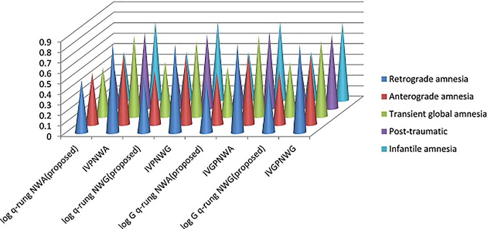
Figure 2: Different Euclidean distance
As shown in Fig. 3, proposed and existing models are compared for HD.
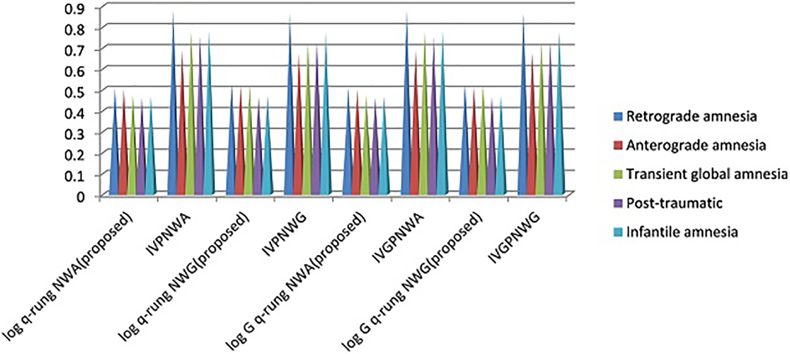
Figure 3: Different Hamming distance
MADM is compared to competing approaches for its merits. A log q-rung NVWA technique is used to derive the various values. Use a log q-rung NVWA operator to generate data for alternatives (q = 2).
Step 1: The aggregated data for each alternative is based on the log q-rung NVWA operators (q = 2). Table 6 represents log q-rung NVWA (q = 2).
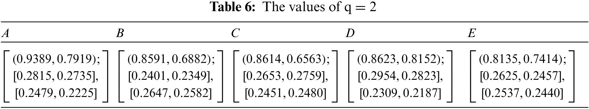
Step 2: In each alternative, the both ideal values are as follows:
and
Step 3: EDs between for all alternative with different ideal values are
and
Step 4: Relative closeness values are
Step 5: Ranking of alternatives are
Step 1: The aggregated data for each alternative is based on the log q-rung NVWA operators (q = 3).
Table 7 represents log q-rung NVWA (q = 3).
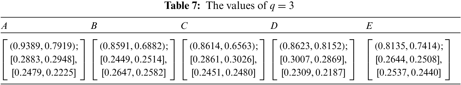
Step 2: In each alternative, the both ideal values are as follows:
and
Step 3: EDs between for all alternative with different ideal values are
and
Step 4: Relative closeness values are
Step 5: Ranking of alternatives are
Fig. 4 shows that different q values for log q-rung NVWA.
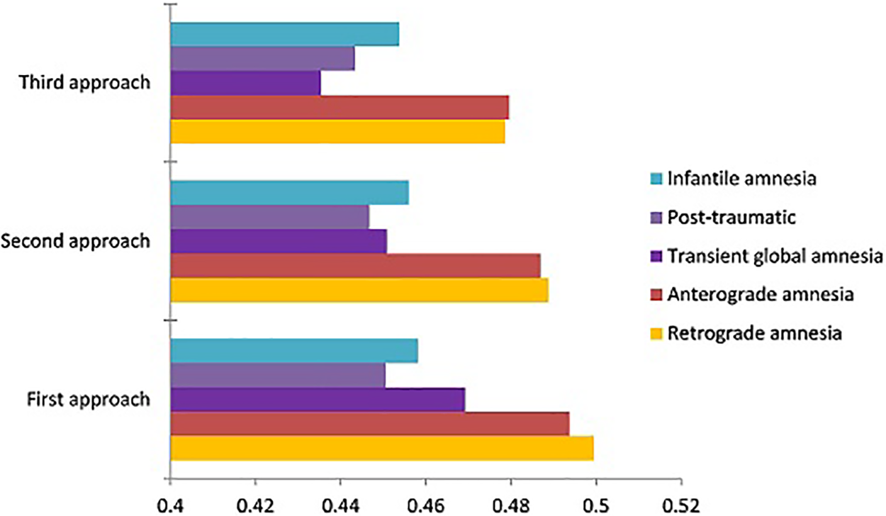
Figure 4: Different q values
On the basis of the log q-rung NVWA method, the alternative would rank as follows: A > C > E > D > B. Assuming that q = 2, then the ranking of alternatives would be A > B > E > C > C. In this case, q = 3, thus the ranking would be B > A > E > D > C. Due to this, the patient is in need of treatment B rather than A. In a similar way, log q-rung NVWGs, log G q-rung NVWAs, and log G q-rung NVWGs can be used.
According to the study previously presented, the applications have numerous advantages. Our research presents the concept of VS and combines it with the concept of q-rung FS to develop a log q-rung VS. The log q-rung NVN analyzes human behaviors and natural events that follow a normal distribution in the real world. The total of its TMG, IMG and FMG exceeds one, but the square sum of those three is less than 1, and so on. A decision maker provides a number of options based on which the proposed log q-rung NVS is used to find the best alternative. As a result, the proposed MADM method that uses log q-rung NVS is another way to find the most effective DM alternative. The outcome of the alternatives based on q. Results of all alternatives obtained using log q-rung NVWAs, log q-rung NVWGs, and log G q-rung NVWAs.
This method is effective due to its ability to consider relationships between attributes. As a result, the proposed method produces more accurate ranking results. Considering the interrelationships between attributes, the proposed method is more efficient and superior to [26] in solving practical DM problems. In this article, we examined problems arising within DM domains using log q-rung NVS and MADM. Based on our discussion of log q-rung NVS, several AO reached a number of conclusions that were important to their log q-rung NVS. There should be a log q-rung NVWA and log q-rung NVWG, as well as a log G q-rung NVWA and log G q-rung NVWG. By applying log q-rung NVS based on the MADM methodology, individuals may be able to determine the appropriate action to take in scenarios with unclear and contradictory facts. We apply the operator representations of log q-rung NVWAs, log q-rung NVWGs, log G q-rung NVWAs and log G q-rung NVWGs to problems based on log q-rung NVS. We can estimate the different rankings using log q-rung NVWA, log q-rung NVWG, log G q-rung NVWA, and log G q-rung NVWG. As a final step, we have examined the values of q that affect alternative ranking most strongly. A decision-maker can select the most appropriate ranking based on a real-world scenario by adjusting q. Based on the actual values of q, the decision-maker can select a method. Finally, we compared the proposed models to a number of currently used models in order to demonstrate their applicability and benefits. In data analysis, HD and ED of neutrosophic sets are used in a number of practical applications. If further research shows that these operators are superior to others, such as power mean aggregation operators, Bonferroni mean operators, Heronian mean operators, etc., we may be able to extend new q-rung complex neutrosophic set to them. The following topics will be discussed in further detail:
(1) It is shown that expert sets and soft sets can be compared with log q-rung NVSs.
(2) The cubic NVS and spherical NVS are investigated on the basis of log q-rung NVSs.
(3) To solve problems with a generalized Fermatean NVS and a complex NVS.
Acknowledgement: Seifedine Kadry would like to thank Dr. Yunyoung Nam for his effort.
Funding Statement: This work was supported by the National Research Foundation of Korea (NRF) Grant funded by the Korea government (MSIT) (No. RS-2023-00218176), Korea Institute for Advancement of Technology (KIAT) Grant funded by the Korea government (MOTIE) (P0012724, The Competency Development Program for Industry Specialist) and the Soonchunhyang University Research Fund.
Author Contributions: The authors confirm contribution to the paper as follows: Conceptualization and methodology: M. Palanikumar; Writing original draft: Nasreen Kausar; Conceptualization: Dragan Pamucar and Chomyong Kim; Validation: Yunyoung Nam; Review and editing: S. Kadry.
Availability of Data and Materials: This statement should make clear how readers can access the data used in the study and explain why any unavailable data cannot be released.
Conflicts of Interest: The authors declare that they have no conflicts of interest to report regarding the present study.
References
1. Zadeh, L. A. (1965). Fuzzy sets. Information and Control, 8(3), 338–353. [Google Scholar]
2. Atanassov, K. (1986). Intuitionistic fuzzy sets. Fuzzy Sets and Systems, 20(1), 87–96. [Google Scholar]
3. Gorzalczany, M. (1987). A method of inference in approximate reasoning based on interval valued fuzzy sets. Fuzzy Sets and Systems, 21, 1–17. [Google Scholar]
4. Biswas, R. (2006). Vague groups. International Journal of Computational Cognition, 4(2), 20–23. [Google Scholar]
5. Yager, R. (2014). Pythagorean membership grades in multi criteria decision-making. IEEE Transactions on Fuzzy Systems, 22, 958–965. [Google Scholar]
6. Peng, X., Yang, Y. (2015). Fundamental properties of interval valued pythagorean fuzzy aggregation operators. International Journal of Intelligent Systems, 31(5), 1–44. [Google Scholar]
7. Ashraf, S., Abdullah, S., Mahmood, T., Ghani, F., Mahmood, T. (2019). Spherical fuzzy sets and their applications in multi-attribute decision making problems. Journal of Intelligent and Fuzzy Systems, 36, 2829–2841. [Google Scholar]
8. Yager, R. R. (2016). Generalized orthopair fuzzy sets. IEEE Transactions Fuzzy Systems, 25(5), 1222–1230. [Google Scholar]
9. Liu, P., Wang, P. (2018). Multiple-attribute decision-making based on archimedean bonferroni operators of q-rung orthopair fuzzy numbers. IEEE Transactions on Fuzzy Systems, 27(5), 834–848. [Google Scholar]
10. Liu, P., Chen, S. M., Wang, P. (2020). Multiple attribute group decision-making based on q-rung orthopair fuzzy power maclaurin symmetric mean operators. IEEE Transactions on System and Cybernetics System, 10(50), 3741–3756. [Google Scholar]
11. Liu, P., Wang, P. (2017). Some q-rung orthopair fuzzy aggregation operators and their applications to multiple-attribute decision making. International Journal of Intelligent Systems, 1, 1–22. [Google Scholar]
12. Wang, P., Liu, P., Chiclana, F. (2021). Multi-stage consistency optimization algorithm for decision making with incomplete probabilistic linguistic preference relation. Information Sciences, 556, 361–388. [Google Scholar]
13. Liu, P., Dang, R., Wang, P., Wu, X. M. (2023). Unit consensus cost-based approach for group decision-making with incomplete probabilistic linguistic preference relations. Information Sciences, 624, 849–880. [Google Scholar]
14. Zhang, C., Ding, J., Li, D., Zhan, J. (2021). A novel multi-granularity three-way decision making approach in q-rung orthopair fuzzy information systems. International Journal of Approximate Reasoning, 138, 161–187. [Google Scholar]
15. Zhang, C., Bai, W., Li, D., Zhan, J. (2022). Multiple attribute group decision making based on multi-granulation probabilistic models, multimoora and tpop in incomplete q-rung orthopair fuzzy information systems. International Journal of Approximate Reasoning, 143, 102–120. [Google Scholar]
16. Zhang, C., Li, D., Kang, X. P., Song, D., Sangaiah, A. K. et al. (2020). Neutrosophic fusion of rough set theory: An overview. Computers in Industry, 115, 103–117. [Google Scholar]
17. Lian, K., Wang, T., Wang, B., Wang, M., Huang, W. et al. (2023). The research on relative knowledge distances and their cognitive features. International Journal of Cognitive Computing in Engineering, 4, 135–148. [Google Scholar]
18. Anusha, G., Ramana, P., Sarkar, R. (2023). Hybridizations of archimedean copula and generalized msm operators and their applications in interactive decision-making with q-rung probabilistic dual hesitant fuzzy environment. Decision Making: Applications in Management and Engineering, 6(1), 646–678. [Google Scholar]
19. Liu, P. D., Teng, F. (2019). Probabilistic linguistic todim method for selecting products through online product reviews. Information Sciences, 485, 441–455. [Google Scholar]
20. Pang, Q., Wang, H., Xu, Z. (2016). Probabilistic linguistic term sets in multi-attribute group decision making. Information Sciences, 369, 128–143. [Google Scholar]
21. Bairagi, B. (2022). A homogeneous group decision making for selection of robotic systems using extended topsis under subjective and objective factors. Decision Making: Applications in Management and Engineering, 5(2), 300–315. [Google Scholar]
22. Cuong, B., Kreinovich, V. (2013). Picture fuzzy sets a new concept for computational intelligence problems. Proceedings of 2013 Third World Congress on Information and Communication Technologies (WICT 2013IEEE, pp. 1–6. [Google Scholar]
23. Liu, W., Chang, J., He, X. (2016). Generalized pythagorean fuzzy aggregation operators and applications in decision making. Control Decision, 2, 2280–2286. [Google Scholar]
24. Rahman, K., Abdullah, S., Shakeel, M., Khan, M., Ullah, M. (2017). Interval valued pythagorean fuzzy geometric aggregation operators and their application to group decision-making problem. Cogent Mathematics, 4, 1–19. [Google Scholar]
25. Rahman, K., Ali, A., Abdullah, S., Amin, F. (2018). Approaches to multi attribute group decision-making based on induced interval valued pythagorean fuzzy einstein aggregation operator. New Mathematics and Natural Computation, 14(3), 343–361. [Google Scholar]
26. Yang, Z., Chang, J. (2020). Interval-valued pythagorean normal fuzzy information aggregation operators for multiple attribute decision making approach. IEEE Access, 8, 51295–51314. [Google Scholar]
27. Fatmaa, K. G., Cengiza, K. (2019). Spherical fuzzy sets and spherical fuzzy topsis method. Journal of Intelligent and Fuzzy Systems, 36(1), 337–352. [Google Scholar]
28. Liu, P., Shahzadi, G., Akram, M. (2020). Specific types of q-rung picture fuzzy yager aggregation operators for decision-making. International Journal of Computational Intelligence Systems, 13(1), 1072–1091. [Google Scholar]
29. Bustince, H., Burillo, P. (1996). Vague sets are intuitionistic fuzzy sets. Fuzzy Sets and Systems, 79, 403–405. [Google Scholar]
30. Kumar, A., Yadav, S. P., Kumar, S. (2007). Fuzzy system reliability analysis using t based arithmetic operations on lr type interval valued vague sets. International Journal of Quality and Reliability Management, 24(8), 846–860. [Google Scholar]
31. Wang, J., Liu, S. J., Zhang, J., Wang, S. Y. (2006). On the parameterized owa operators for fuzzy mcdm based on vague set theory. Fuzzy Optimization and Decision Making, 5, 5–20. [Google Scholar]
32. Zhang, X., Xu, Z. (2014). Extension of topsis to multiple criteria decision-making with pythagorean fuzzy sets. International Journal of Intelligent Systems, 29, 1061–1078. [Google Scholar]
33. Jana, C., Pal, M. (2018). Application of bipolar intuitionistic fuzzy soft sets in decision-making problem. International Journal of Fuzzy System Applications, 7(3), 32–55. [Google Scholar]
34. Ullah, K., Mahmood, T., Ali, Z., Jan, N. (2019). On some distance measures of complex pythagorean fuzzy sets and their applications in pattern recognition. Complex and Intelligent Systems, 6, 15–27. [Google Scholar]
35. Jana, C., Pal, M. (2021). Multi criteria decision-making process based on some single valued neutrosophic dombi power aggregation operators. Soft Computing, 25(7), 5055–5072. [Google Scholar]
36. Palanikumar, M., Iampan, A. (2022). Spherical fermatean interval valued fuzzy soft set based on multi criteria group decision making. International Journal of Innovative Computing, Information and Control, 18(2), 607–619. [Google Scholar]
37. Palanikumar, M., Iampan, A. (2022). Novel approach to decision making based on type-II generalized fermatean bipolar fuzzy soft sets. International Journal of Innovative Computing, Information and Control, 18(3), 769–782. [Google Scholar]
38. Yang, M. S., Ko, C. H. (1996). On a class of fuzzy c-numbers clustering procedures for fuzzy data. Fuzzy Sets and Systems, 84, 49–60. [Google Scholar]
39. Xu, R. N., Li, C. L. (2001). Regression prediction for fuzzy time series. Applied Mathematics-A Journal of Chinese Universities, 16, 451–461. [Google Scholar]
40. Jin, Y., Ashraf, S., Abdullah, S. (2019). Spherical fuzzy logarithmic aggregation operators based on entropy and their application in decision support systems. Entropy, 21, 1–36. [Google Scholar]
41. Ashraf, S., Abdullah, S., Smarandache, F. (2019). Logarithmic hybrid aggregation operators based on single valued neutrosophic sets and their applications in decision support systems. Symmetry, 11, 364–376. [Google Scholar]
42. Palanikumar, M., Arulmozhi, K., Jana, C. (2022). Multiple attribute decision-making approach for pythagorean neutrosophic normal interval-valued aggregation operators. Computational and Applied Mathematics, 41(90), 1–27. [Google Scholar]
43. Peng, X., Yuan, H. (2016). Fundamental properties of pythagorean fuzzy aggregation operators. Fundamenta Informaticae, 147, 415–446. [Google Scholar]
44. Adak, A. K., Kumar, G. (2023). Spherical distance measurement method for solving mcdm problems under pythagorean fuzzy environment. Journal of Fuzzy Extension & Applications, 4(1), 28–39. [Google Scholar]
45. Hasan, M. K., Ali, M. Y., Sultana, A., Mitra, N. K. (2022). Some picture fuzzy mean operators and their applications in decision-making. Journal of Fuzzy Extension & Applications, 3(4), 349–361. [Google Scholar]
46. Mishra, V. N., Kumar, T., Sharma, M. K., Rathour, L. (2023). Pythagorean and fermatean fuzzy sub-group redefined in context of T-norm and S-conorm. Journal of Fuzzy Extension & Applications, 4(2), 125–135. [Google Scholar]
47. Abbas, M., Asghar, M. W., Guo, Y. (2022). Decision-making analysis of minimizing the death rate due to COVID-19 by using q-rung orthopair fuzzy soft bonferroni mean operator. Journal of Fuzzy Extension & Applications, 3(3), 231–248. [Google Scholar]
48. Yaman, T. T., Akkartal, G. R. (2022). How warehouse location decisions changed in medical sector after pandemic? A fuzzy comparative study. Journal of Fuzzy Extension & Applications, 3(1), 81–95. [Google Scholar]
49. Limboo, B., Dutta, P. (2022). A q-rung orthopair basic probability assignment and its application in medical diagnosis. Decision Making: Applications in Management and Engineering, 5(1), 290–308. [Google Scholar]
50. Ranjan, M. J., Kumar, B. P., Bhavani, T. D., Padmavathi, A. V., Bakka, V. (2023). Probabilistic linguistic q-rung orthopair fuzzy archimedean aggregation operators for group decision-making. Decision Making: Applications in Management and Engineering, 6(2), 639–667. [Google Scholar]
51. Riaz, M., Farid, A. H. M. (2022). Picture fuzzy aggregation approach with application to third-party logistic provider selection process. Reports in Mechanical Engineering, 3(1), 227–236. [Google Scholar]
52. Khan, M. R., Ullah, K., Khan, Q. (2023). Multi-attribute decision-making using archimedean aggregation operator in t-spherical fuzzy environment. Reports in Mechanical Engineering, 4(1), 18–38. [Google Scholar]
53. Mahmood, T., Rehman, U. (2023). Bipolar complex fuzzy subalgebras and ideals of BCK/BCI-algebras. Journal of Decision Analytics and Intelligent Computing, 3(1), 47–61. [Google Scholar]
54. Sahoo, S. K., Goswami, S. S. (2023). A comprehensive review of multiple criteria decision-making (MCDM) methods: Advancements, applications, and future directions. Decision Making Advances, 1(1), 25–48. [Google Scholar]
55. Naseem, A., Akram, M., Ullah, K., Ali, Z. (2023). Aczel-alsina aggregation operators based on complex single-valued neutrosophic information and their application in decision-making problems. Decision Making Advances, 1(1), 86–114. [Google Scholar]
Appendix
Proof of the Theorem 4.1
Proof. It is clear that (1) and (2) can be proven. There is only one proof we provide for the last statement (3). Now,
where
Proof of the Theorem 5.1
Proof. This theorem is proven by using the induction method. If n = 2, then log q-rung NVWA
and
Hence,
Thus, log q-rung NVWA
It valid for n = l and l
If n = l + 1, then log q-rung NVWA
Proof of the Theorem 5.2
Proof. Given that
Proof of the Theorem 5.3
Proof. Since,
Since,
Since,
Hence,
Proof of the Theorem 5.4
Proof. For any i,
Hence, log q-rung NVWA
Proof of the Theorem 5.7
Proof. We prove that,
It valid for n = l and l
Thus,
Hence,
A log G q-rung NVWA operator is modified into a log G q-rung NVWA operator when q = 1 is specified.
Cite This Article
 Copyright © 2024 The Author(s). Published by Tech Science Press.
This work is licensed under a Creative Commons Attribution 4.0 International License , which permits unrestricted use, distribution, and reproduction in any medium, provided the original work is properly cited.
 Downloads
 Citation Tools