Full-Scale Isogeometric Topology Optimization of Cellular Structures Based on Kirchhoff–Love Shells

Nomenclature

1  Introduction

Thin-shell structures are widely applied in the aerospace [1], automobile [2] and civil engineering [3] fields due to their excellent load-carrying capacity. The mechanical behavior of a thin-shell structure can be described by shell elements based on surface models because the thickness of the thin-shell structure is much smaller than its size in the other directions. Reissner–Mindlin [4] and Kirchhoff–Love [5] models are the two most widely used mathematical models for describing shells. Reissner–Mindlin theory considering the transverse shear force is primarily used to describe thick shells. It is very suitable for the finite element method (FEM) based on the C0-continuous Lagrangian basis function since the shell elements in this theory need to ensure only C0-continuity. Therefore, the Reissner–Mindlin shell model is widely used in most current industrial software. In contrast, Kirchhoff–Love theory describes thin shells based on the assumption that the shell is thin enough to neglect transverse shear deformation. The rotation of the shell is described by the first derivative of displacement; hence, at least the C1-continuity of the shell elements must be guaranteed in Kirchhoff–Love theory [6]. Because the FEM has difficulty constructing C1-continuous elements, Kirchhoff–Love theory is rarely adopted in current mainstream industrial software.

Compared with FEM, isogeometric analysis (IGA) [7] can avoid remeshing via the same basis function to describe the geometric structure and construct the analysis grid, hence eliminating geometric approximation errors by unifying geometric and analysis models of structures and attracting widespread concern [8]. NURBS basis functions are the most widely used functions in IGA due to their geometric flexibility and high-order continuity. Because nonuniform rational B-splines (NURBS) is convenient for constructing high-order continuous mesh elements, which aligns with Kirchhoff–Love theory’s requirement for the C1-continuity of shell elements, IGA is suitable for use with the Kirchhoff–Love shell theory. Kiendl et al. [9] developed a Kirchhoff–Love shell element based on IGA, which was applied in thin shells under large rotation by a geometrically nonlinear formulation. Guo et al. [10] proposed a variationally consistent weak coupling method for thin-walled shell patches based on IGA, which ensured the effective transfer of the displacement and bending moment between multiple NURBS patches. This method enabled a blended coupling of shells based on different mathematical models, such as Kirchhoff–Love and solid-like shell models. Li et al. [11] presented a novel method coupling the meshfree method and IGA for geometrically nonlinear analysis of thin-shell structures based on Kirchhoff–Love theory. Thanh et al. [12] further extended the above method to static and free-vibration analyses of cracks in thin-shell structures, and Zhang et al. [13] coupled the isogeometric–meshfree method with the peridynamic method for static and dynamic crack propagation. Hirschler et al. [14] proposed a dual domain decomposition algorithm to address the inconsistencies between multiple NURBS patches for accurately analyzing nonconforming multipatch Kirchhoff–Love shells. Zareh et al. [15] developed isogeometric Kirchhoff–Love shell elements based on Cr smooth rational triangular Bézier splines. These elements overcame limitations on complex geometries requiring multiple NURBS patches, offering a more efficient way to handle complex geometric models. Miao et al. [16] developed an isogeometric Bézier dual mortar method coupling multipatch Kirchhoff–Love shells, which strengthened the continuity of the solution at the boundaries of patches. Peng et al. [17] developed a novel continuum-based fast projection scheme for cloth simulation based on the isogeometric Kirchhoff–Love shell model. Current methods for Kirchhoff–Love shell analysis based on IGA have applications in various emerging research areas, such as metamaterials [18], hyperelastic materials [19], biomechanics [20], lattice shells [21], and optimization of stiffeners for thin shell structures [22].

Topology optimization [23], as an effective structural design method, can enable the performance potential of structures to be fully explored by iteratively finding the optimal distribution of materials in the design domain under given design constraints and objectives. Through topology optimization, unprecedented thin-shell structures that extend beyond the experience and intuition of designers can be generated to further improve the strength-to-weight ratio, hence achieving ultralightweight designs and obtaining broad application prospects [24]. Recently, the combination of IGA and topology optimization, i.e., isogeometric topology optimization (ITO), has attracted great attention. Hassani et al. [25] proposed an ITO method, in which a solid isotropic material with penalization (SIMP) method based on control points was employed. Wang et al. [26] proposed an ITO method based on the level set method (LSM), in which NURBS basis functions were used to construct physical fields and to parameterize level set functions. Gao et al. [27] developed an ITO method based on a smooth density distribution function, in which the Shepard function was used to construct a smooth density distribution function, which was employed to ensure that the structural boundary of the optimized result was clear and smooth. Zhu et al. [28] presented an explicit ITO based on graded truncated hierarchical B-splines. Meanwhile, some studies on the applications of ITO to shell structures have also been conducted. Kang et al. [29] proposed an ITO method for shell structures, in which trimmed surface analysis was used to handle complex topologies. Zhang et al. [30] presented an ITO method for a 3D shell under stress constraints, in which the moving morphable voids method was adopted to explicitly describe the topological configuration.

Additionally, multiscale topology optimization is widely employed for cellular structure design to achieve extraordinary performances, such as excellent dynamic behavior [31], high stiffness-to-weight ratio [32,33] and fast heat dissipation [34]. The majority of multiscale topology optimization methods utilize the homogenization theory based on scale separation and periodic assumptions to establish the relationship between macro and micro scales [35]. The geometry of the micro structures filling in the cellular structure is generally limited to regular shapes, such as squares and parallelograms. As a result, few investigations have been conducted on the topology optimization design of cellular structures with curved edges or surfaces by homogenization theory [36]. Another strategy for designing cellular structures is the full-scale topology optimization method [37]. Full-scale topology optimization generates many bone-like holes by imposing local volume constraints within the design domain without using homogenization theory. Therefore, this full-scale topology optimization method can be used to design irregular cellular structures with curved edges or surfaces.

Based on these considerations, a high-order continuous Kirchhoff–Love shell model based on IGA is proposed, and a cellular thin-shell structure with high damage robustness is designed via full-scale ITO. NURBS is used to describe the geometry of the shell and establish its analysis model to improve the analysis accuracy. A density field is built on the control mesh to describe the topological configuration of the shell. Local volume constraints, which are aggregated into an equivalent global constraint by the p-norm function, are introduced into ITO to obtain bone-like thin-shell structures. The simulation and comparison of several numerical examples show that the cellular thin-shell structures obtained by the proposed method have great bearing capacity and damage robustness.

The remainder of the paper is organized as follows: Section 2 describes the full-scale ITO model based on the Kirchhoff–Love shell in detail. Section 3 provides the numerical implementation and framework. Section 4 provides several numerical examples to verify the effectiveness of the proposed method and the excellent performances of the structures optimized by the proposed method. Section 5 summarizes and discusses the research work of this paper.

2  Full-Scale Isogeometric Topology Optimization Based on the Kirchhoff–Love Shell

2.1 Local Volume Constraint

To generate a bone-like cellular structure on a thin shell, the local volume constraint method is introduced [37]. The average of the effective densities in the designated neighborhood nc of each control point is taken as the local volume fraction Lc of the current control point c. Lc is calculated as follows:

Lc=∑i∈ncρi∑i∈nc1(1)

where ρi represents the density of the control point in the designated neighborhood nc, where nc represents the set of adjacent control points of the current control point. The distance between adjacent control points and the current control point must be less than the specified influence radius r, as follows:

nc={i|||Pi−Pc||2≤r}(2)

where Pc is the coordinate of the current control point and Pi is the coordinate of the adjacent control point. The local volume constraint is represented as follows:

gc=Lc≤Lmax,c=1,2,…,Nc(3)

where gc represents the local volume constraint of the c th control point, Lmax denotes the specified upper limit of the local volume fraction, and Nc denotes the total number of control points. Imposing a local volume constraint on each control point results in many constraints, and implementing these constraints is difficult. These constraints can be represented by an aggregated constraint max(Lc)≤Lmax. Since the aggregated constraint is nondifferentiable, the p-norm function is used to approximate the max function as follows:

max(Lc)≈‖L‖p=(∑c(Lc)p)1p(4)

When p tends to infinity, ||L||p is completely equivalent to max(Lc). If p is not infinite, the aggregated constraint can be written as:

g=(∑c(Lc)p)1p≤(∑c(Lmax)p)1p,c=1,2,…,Nc(5)

The size of p determines how strict the local volume constraint is.

2.2 Full-Scale ITO Model

In the full-scale design framework, an ITO model for the cellular thin-shell structure is established with the minimum compliance as the objective function and the global and local volume fractions as constraints, as follows:

Find:ρi(i=1,2,…,Nc)Min:J(ρi)=∫ΩueTK~e(ρi)uedΩ

s.t.:{K(ρi)u=fG(ρi)=1|Ω|∫Ωx(ρi)νdΩ−Vmax≤0g(ρi)=(∑c(Lc(ρi))p)1p≤(∑c(Lmax)p)1p0<ρmin≤ρi≤1(6)

where ρi is the effective density at the Nc control point, namely, the design variable. J denotes the objective function, that is, the minimum compliance. ue is the element displacement, and Ω is the design domain of the thin shell. K is the global stiffness matrix, u is the displacement vector, and f is the force load vector. The equilibrium equation is constructed by the Kirchhoff–Love model based on IGA. G(ρi) represents the global volume constraint, Vmax represents the specified upper limit of the global volume fraction, and ν represents the element volume. g(ρi) represents the aggregated local volume constraint. ρmin represents the lower limit of the design variable. K~e(ρi) represents the interpolated element stiffness matrix [23] and is calculated as follows:

K~e(ρi)=x(ρi)Ke(7)

where x(ρi) is the effective density field constructed by the effective density ρi on the control point and the corresponding NURBS basis function Ri. x(ρi) is expressed as follows:

x(ρi)=∑i=1nRi(ϕi(ρi))τ(8)

where τ denotes the penalty factor, and n represents the number of control points, which is the number of effective densities. ϕi(ρi) represents the Heaviside step function [38], written as:

ϕi(ρi)=tanh⁡(σ2)+tanh⁡(σ(ρi−12))2tan⁡h(σ2)(9)

where σ represents the projection parameter to control the sharpness of the Heaviside step function. The Heaviside step function is adopted to promote the generation of the 0–1 solution. The larger the σ value is, the more the effective density field obtained by the Heaviside step function tends toward being a 0–1 distribution. However, directly applying a large σ can result in highly nonlinear equations. To ensure the stability of the iteration process, σ is initialized as σ=1, and value is doubled after every 50 iterations until σ=16. This is a commonly used technique for promoting convergence in topology optimization [38]. The effective density of any point on the shell can be obtained through the effective density field x(ρi), which reflects whether each point on the shell corresponds to solid material or void. The topological configuration of the shell is optimized by optimizing the reasonable distribution of effective density.

2.3 NURBS Basis Functions

To construct NURBS basis functions, first, the B-spline basis function with a monotonically increasing open knot vector Ξ={ξ1,ξ2,⋯,ξn+p+1} is expressed by the recursive formula [8], as follows:

{Ni,0(ξ)={1, ifξi≤ξ<ξi+10, otherwise,p=0Ni,p(ξ)=ξ−ξiξi+p−ξiNi,p−1(ξ)+ξi+p+1−ξξi+p+1−ξi+1Ni+1,p−1(ξ),p≥1(10)

where n and p represent the number and degree of B-spline basis functions, respectively. The knot vector represents the coordinates of the element nodes in the parametric domain, and the knot spans represent the elements. Then, introducing the weight ωi yields the NURBS basis functions as follows:

Rip(ξ)=Ni,p(ξ)ωi∑i^=1nNi^,p(ξ)ωi^(11)

where ωi is the weight. Furthermore, a NURBS curve can be written as:

Curve(ξ)=∑i=1nRip(ξ)Pi(12)

where Pi is the coordinate of the control point corresponding to the NURBS basis function. Similarly, a NURBS surface can be described by the tensor product of the NURBS basis functions in directions ξ and η, written as:

Surf(ξ,η)=∑i=1n∑j=1mRi,jp,q(ξ,η)Pi,j(13)

where n and m are the number of control points in two parametric directions, and p and q are the corresponding polynomial degrees. Specifically, Ri,jp,q is written as follows:

Ri,jp,q(ξ,η)=Ni,p(ξ)Nj,q(η)ωij∑i^=1n∑j^=1mNi^,p(ξ)Nj^,q(η)ωi^j^(14)

where Ni,p(ξ) and Nj,q(η) represent B-spline basis functions in two parametric directions.

2.4 Kirchhoff–Love Shell Model

In this paper, the IGA-based Kirchhoff–Love model is used to analyze the mechanical behavior of the thin shell. First, the three-dimensional shell is described with the curvilinear coordinate (ξ1,ξ2,ξ3), where ξ1 and ξ2 represent the in-plane directions, and ξ3 represents the shell thickness direction. As shown in Fig. 1, the position vectors x and X of any point in the shell in the current and reference configurations, respectively, are represented as follows [39]:

x(ξ1,ξ2,ξ3)=r(ξ1,ξ2)+ξ3a3(ξ1,ξ2)X(ξ1,ξ2,ξ3)=R(ξ1,ξ2)+ξ3A3(ξ1,ξ2)(15)

where r and R represent the position vectors of any point of the mid-surface in the current and reference configurations, respectively. a3 and A3 represent the unit director vectors of the mid-surface in the current and reference configurations, respectively, defined as follows:

{a3=a1×a2|a1×a2|aα=r,α=∂r∂ξα and {A3=A1×A2|A1×A2|Aα=R,α=∂R∂ξα(16)

where aα and Aα represent the covariant basis vectors of the mid-surface in the current and reference configurations, respectively. Here, the Greek index α = 1, 2. The corresponding inverse basis vectors aα and Aα are defined as follows:

aα⋅aβ=Aα⋅Aβ=δβα(17)

where δβα represents the Kronecker delta. Therefore, the covariant metric coefficients and the inverse metric coefficients of the mid-surface in the current and reference configurations are expressed as follows:

{aij=ai⋅ajaij=[aij]−1and{Aij=Ai⋅AjAij=[Aij]−1(18)

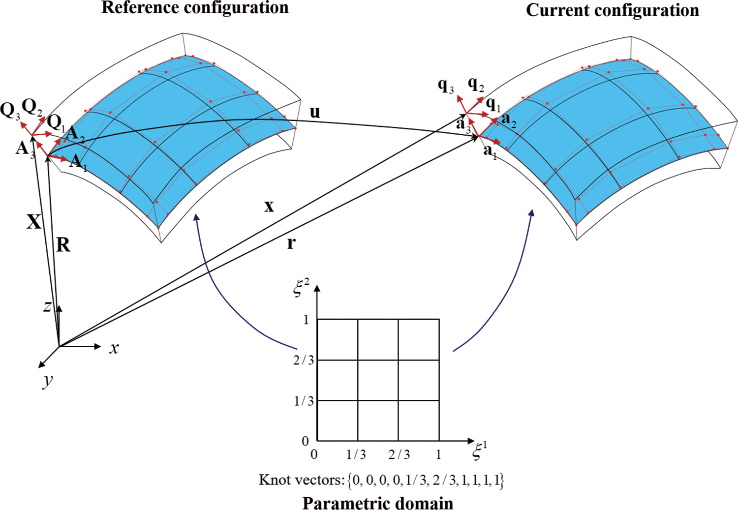
Figure 1: Geometric description of the Kirchhoff–Love shell. The mid-surface is highlighted in blue, red points represent control points, and red dashed lines represent the control mesh. The knot vectors are {0,0,0,0,1/3,2/3,1,1,1,1} in two parametric directions

The displacement vector u of the mid-surface between the current and reference configurations is calculated as follows:

u(ξ1,ξ2)=r(ξ1,ξ2)−R(ξ1,ξ2)(19)

The covariant basis vectors at any material point in the current and reference configurations are defined as follows:

{qα=x,α=aα+ξ3a3,αq3=x,3=a3 and {Qα=X,α=Aα+ξ3A3,αQ3=X,3=A3(20)

Similarly, the corresponding inverse basis vectors qα and Qα are defined as follows:

qα⋅qβ=Qα⋅Qβ=δβα(21)

The covariant metric coefficients and the inverse metric coefficients at any material point in the current and reference configurations are expressed as follows:

{qij=qi⋅qjqij=[qij]−1and{Qij=Qi⋅QjQij=[Qij]−1(22)

Based on Kirchhoff–Love’s hypothesis, the Green-Lagrange strain tensor [40] can be written as:

E=EαβQα⊗Qβ(23)

where

Eαβ=12(qαβ−Qαβ)(24)

Bringing Eqs. (22) into (24) yields

Eαβ=εαβ+ξ3καβ(25)

where εαβ and καβ represent the membrane strain and bending strain, respectively, as follows:

{εαβ=12(aα⋅aβ−Aα⋅Aβ)καβ=−aα,β⋅a3+Aα,β⋅A3(26)

Next, the strain energy density per unit area of the Kirchhoff–Love shell can be expressed as:

W(ξ1,ξ2)=12(tε:C:ε+t312κ:C:κ)(27)

where t is the shell thickness. C is the material tensor, written as:

C=CαβγδAα⊗Aβ⊗Aγ⊗Aδ,Cαβγδ=Eν1−ν2AαβAγδ+E2(1+ν)(AαγAβδ+AαδAβγ)(28)

where E is Young’s modulus and ν is Poisson’s ratio.

2.5 Governing Equations and Discretization in IGA

The potential energy of the Kirchhoff–Love shell can be calculated by the following formula:

Π(u)=Πint(u)+Πext(f,u)=∫Ω¯WdΩ+Πext(f,u)(29)

where Ω¯ is the mid-surface of the shell in the reference configuration. Πint(u) is the strain energy, and Πext(f,u) is the external work generated by the external force f. According to the principle of virtual work, the displacement variable u must meet the balance condition of potential energy minimization:

δΠ=∂Π∂uδu=∫Ω¯δε(u,δu):n(u)+δκ(u,δu):m(u)dΩ+Πext(f,u)=0(30)

where δε and δκ represent the first variation of membrane and bending strains. n and m represent the membrane force resultant tensor and bending moment tensor, respectively, and are expressed as:

{n=nαβAα⊗Aβ,nαβ=∂W∂εαβ=tCαβγδεγδm=mαβAα⊗Aβ,mαβ=∂W∂καβ=t312Cαβγδκγδ(31)

Eq. (30) is solved iteratively. Assuming ui+1=ui+Δu, the variational Eq. (30) is linearized as follows: Find Δu∈U¯ such that

Km(ui,δu,Δu)+Kb(ui,δu,Δu)=−δΠ(ui,δu),∀δu∈U¯(32)

where Km and Kb are the membrane stiffness and bending stiffness, respectively, and are expressed as:

Km(ui,δu,Δu)=∫Ω¯δε(u,δu):δn(u,Δu)+δε(u,δu,Δu):n(u)dΩKb(ui,δu,Δu)=∫Ω¯δκ(u,δu):δm(u,Δu)+δκ(u,δu,Δu):m(u)dΩ(33)

Eq. (32) can be converted into a discrete equation by numerical integration:

Ku=f(34)

where K is the positive definite stiffness matrix, u is the displacement vector, and f is the force load vector. Eq. (34) is also the equilibrium equation in Eq. (6). Furthermore, in IGA, u is expressed by the linear combination of the displacement ui,j at the control point and the corresponding NURBS basis function Ri,jp,q, as follows:

u(ξ1,ξ2)=∑i=1n∑j=1mRi,jp,q(ξ1,ξ2)ui,j(35)

Similarly, the coordinates r(ξ1,ξ2) of any point on the mid-surface of the shell can be expressed as:

r(ξ1,ξ2)=∑i=1n∑j=1mRi,jp,q(ξ1,ξ2)ri,j(36)

The stiffness matrix K is composed of the element stiffness matrix Ke. Ke is composed of the element membrane stiffness matrix Kem and element bending stiffness matrix Keb, as follows:

Ke=∑i=13∑j=13{(Kem+Keb)|J1||J2|ωij}=∑i=13∑j=13{[t(Bm)TCeBm+t312(Bb)TCeBb]|J1||J2|ωij}(37)

where Ce is the element material tensor, Bm is the membrane strain-displacement matrix, and Bb is the bending strain-displacement matrix. 3 × 3 Gauss-quadrature points are selected in each element to calculate the element stiffness matrix. ωij is the weight of the Gauss-quadrature point in each element. J1 is the Jacobian matrix mapped from the parametric domain to the physical domain, and J2 is the Jacobian matrix mapped from the parent domain to the parametric domain. Here, Gauss-Legendre quadrature rules are employed for numerical integration in IGA.

3  Numerical Implementation and Framework

3.1 Sensitivity Analysis

Since the above full-scale ITO model involves multiple constraint functions, method of moving asymptotes (MMA) algorithm is adopted to update the design variables [41]. The MMA method requires calculating the sensitivity of the objective function and constraints. The sensitivity of the objective function J(ρi) with respect to the design variable ρi is calculated as follows:

∂J(ρi)∂ρi=ueT∂K~e(ρi)∂ρiue=∂x(ρi)∂ρiueTKeue(38)

where ∂x(ρi)∂ρi is calculated according to Eqs. (8) and (9) as follows:

∂x(ρi)∂ρi=τRi(ϕi(ρi))τ−1⋅σ[1−tanh2⁡(σ(12−ρi))]2tan⁡h(σ2)(39)

Using the chain rule, the sensitivity of local volume constraint g(ρi) with respect to design variable ρi is calculated as follows:

∂g(ρi)∂ρi=∂g(ρi)∂Lj(ρi)⋅∂Lj(ρi)∂ρi(40)

Using Eqs. (5) and (1), ∂g(ρi)∂Lj(ρi) and ∂Lj(ρi)∂ρi are calculated as follows:

{∂g(ρi)∂Lj(ρi)=(∑c⁡(Lc(ρi))p)1p−1⋅(Lj(ρi))p−1∂Lj(ρi)∂ρi=1∑j∈nc1(41)

Similarly, the sensitivity of the global volume constraint G(ρi) with respect to the design variable ρi is as follows:

∂G(ρi)∂ρi=1|Ω|ν⋅∂x(ρi)∂ρi=1|Ω|ν⋅τRi(ϕi(ρi))τ−1⋅σ[1−tanh2⁡(σ(12−ρi))]2tanh⁡(σ2)(42)

3.2 Optimization Design Framework

The optimization design framework of the cellular thin-shell structure is shown in Fig. 2. The specific steps of the framework are as follows:

Step 1: Construct the design domain of the thin shell based on the NURBS basis function and set boundary conditions;

Step 2: Construct the effective density field and local volume fraction field;

Step 3: Compute the displacement field of the thin-shell structure by IGA;

Step 4: Calculate the objective function and constraints and conduct sensitivity analysis;

Step 5: Update effective densities by the MMA method;

Step 6: If the maximum change in effective density between two iterations is less than 1% or the number of iteration steps reaches 800, stop the iteration; otherwise, repeat steps 3-6;

Step 7: Output the optimized result to obtain the final cellular thin-shell structure.

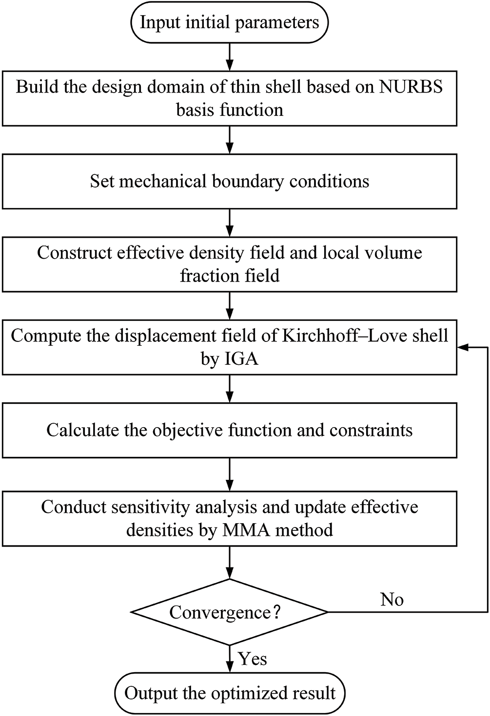
Figure 2: Optimization flow chart

4  Numerical Examples

In this section, several numerical examples are provided to demonstrate the effectiveness of the proposed method. Unless otherwise specified, stainless steel material with Young’s modulus E = 200 GPa and Poisson’s ratio v = 0.3 is used in all examples. The upper limits of the global and local volume constraints are set to 0.5 and 0.6, respectively. Both the penalty factor and the filter radius are set to 3.

4.1 Scordelis–Lo Roof

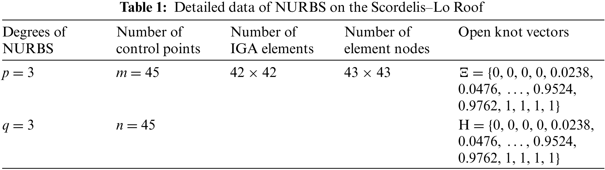
First, a benchmark example is used to verify the accuracy of the proposed method. Fig. 3 displays the design domain of the Scordelis–Lo Roof, a very popular and extremely severe example. Fig. 4 shows the IGA mesh of the Scordelis–Lo Roof. The thickness of the shell is 0.25 mm. Two curved edges are fixed, and a uniform vertical load F = 90 N is imposed on the entire shell. To align with the standard description of this benchmark problem, the material properties are set to Young’s modulus E = 432 MPa and Poisson’s ratio v = 0 here. The detailed data of the NURBS on the Scordelis–Lo Roof are displayed in Table 1.

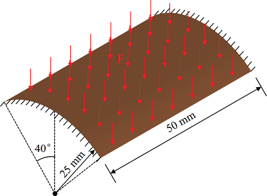
Figure 3: Design domain of the Scordelis–Lo Roof

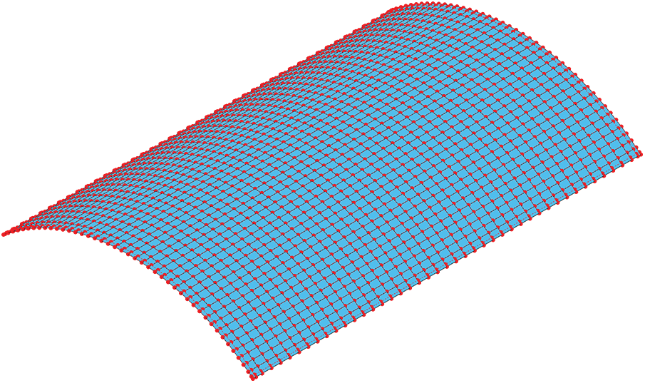
Figure 4: IGA mesh of the Scordelis–Lo Roof

The vertical displacement field obtained by the proposed method is shown in Fig. 5. The maximum vertical displacement of the middle side calculated by the proposed method is 0.3077, which is close to the reference solution of 0.3086 in [42] and the solution of 0.308 in [15]. Hence, the accuracy of the proposed method is demonstrated through this benchmark example of the Scordelis–Lo Roof.

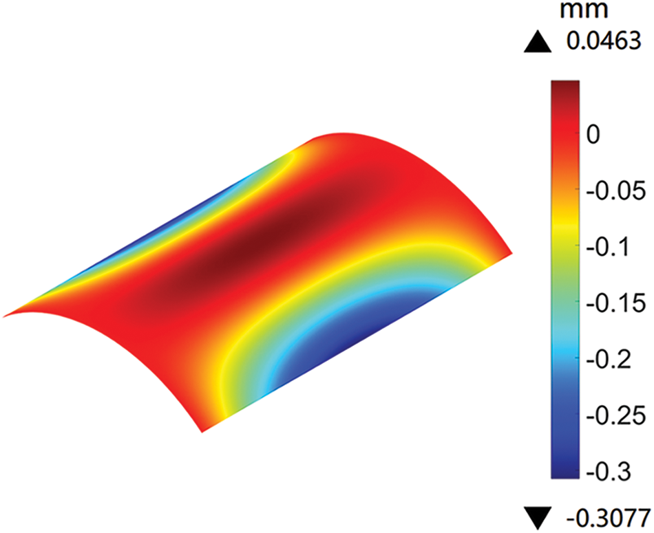
Figure 5: Vertical displacement field of the Scordelis–Lo Roof obtained by the proposed method

4.2 Blunt Cone Shell

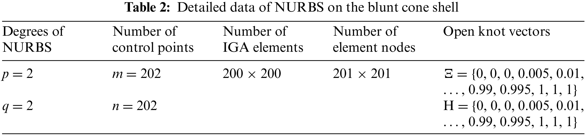
A design domain of a blunt cone shell is shown in Fig. 6. The four corners of the blunt cone shell are fixed, and a vertical downward force load F = 100 N is applied at its center point. The thickness of the thin shell is 1 mm. The design domain of the blunt cone shell is divided into 200 × 200 IGA elements for topology optimization, as shown in Fig. 7. The parameters of the corresponding IGA mesh are provided in Table 2. In the optimization model, the influence radius of the local volume fraction is set to 10.

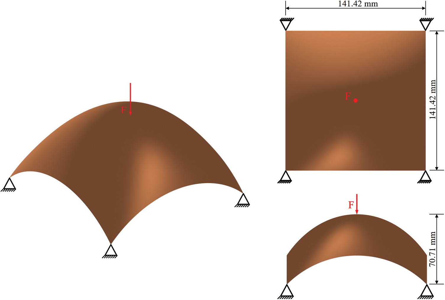
Figure 6: Design domain of the blunt cone shell

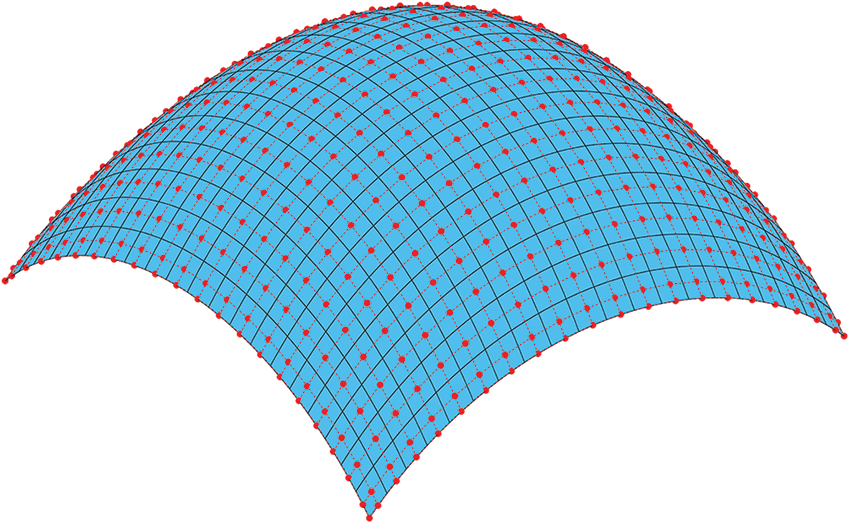
Figure 7: IGA mesh of the blunt cone shell, where the mesh resolution is set to one-tenth of the actual resolution for better visualization

To verify the analysis results of IGA, the analysis result of the blunt cone shell obtained by the commercial FEM software COMSOL is compared with that obtained by IGA. By importing the STL file of the blunt cone shell into COMSOL, the same geometric modeling can be obtained. Fig. 8 depicts the displacement fields obtained by IGA and COMSOL. Here, the number of elements of IGA is set to 50 × 50 to demonstrate the analysis accuracy of IGA, while the number of elements in COMSOL is 7942. Comparison reveals that the contour lines of the two displacement fields by IGA and COMSOL are almost identical. Meanwhile, the maximum displacements of the analysis results of the two methods are very similar. Therefore, this comparison illustrates that IGA requires fewer elements to achieve the same level of accuracy as the FEM.

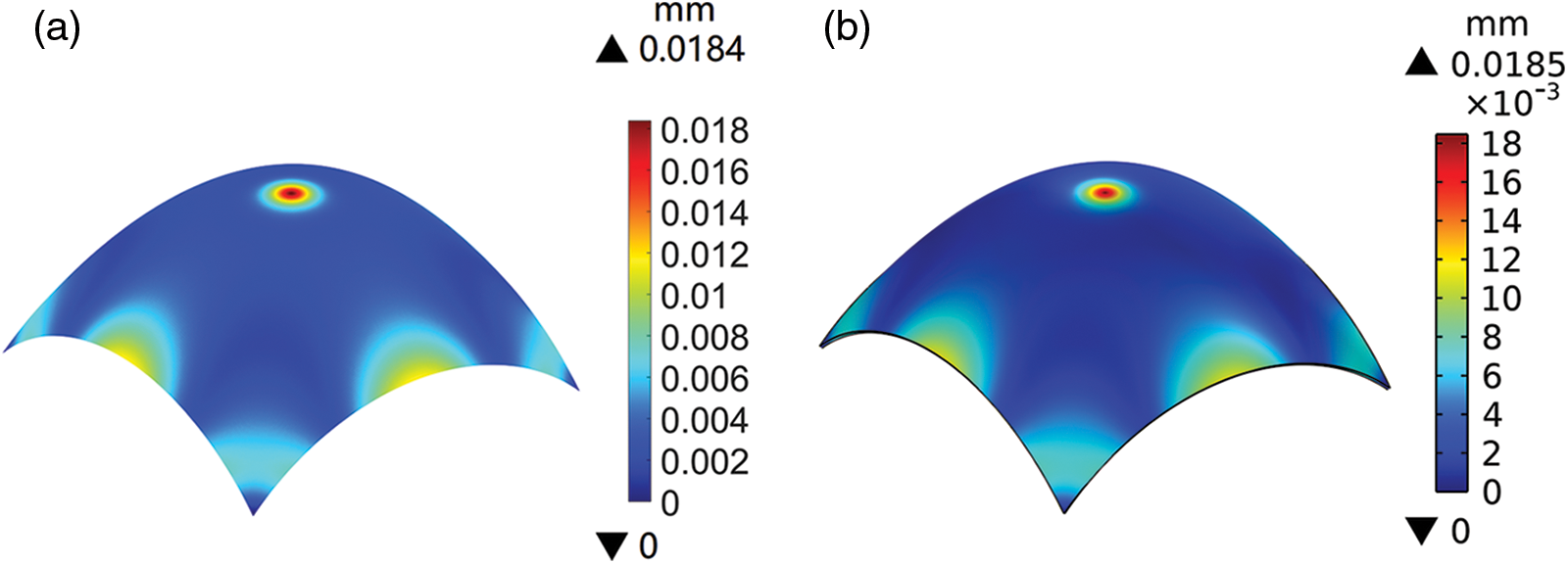
Figure 8: Displacement fields of the blunt cone shell: (a) by IGA; (b) by COMSOL

The iteration curves of the blunt cone shell are shown in Fig. 9. The iteration curves fluctuate significantly in the first 200 steps due to σ in the Heaviside function doubling every 50 steps, as described in Section 2.2. After 200 iterations, the iteration curves are stable, and the compliance reaches the minimum while meeting the volume constraint. Fig. 10 displays the final optimized result, namely, the optimized effective density distribution. Many small voids are produced in the optimized results due to local volume constraints. The material is primarily distributed along the main force transmission path from the load application point at the center of the blunt cone shell to the four fixed corners.

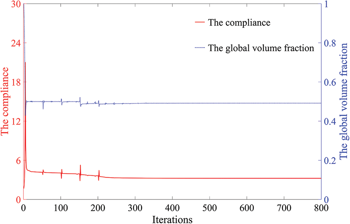
Figure 9: Iteration curves of the blunt cone shell

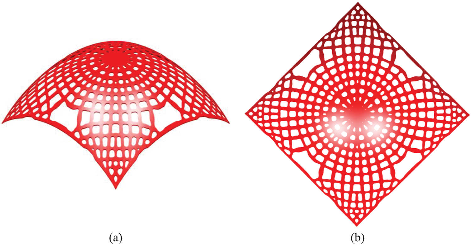
Figure 10: Optimized result of the blunt cone shell: (a) optimized cellular thin-shell structure; (b) top view of the cellular thin-shell structure

The influences of different parameters on the optimized result are also discussed through this numerical example. Fig. 11 shows four optimized results under different upper limits Lmax of the local volume constraint and influence radius r. The upper limit of the local volume constraint controls the local porosity, while the influence radius affects the size of the holes. The larger the influence radius is, the larger the size of the holes. Therefore, the size of the holes in the optimized result can be controlled by adjusting the upper limit of the local volume constraint and the influence radius.

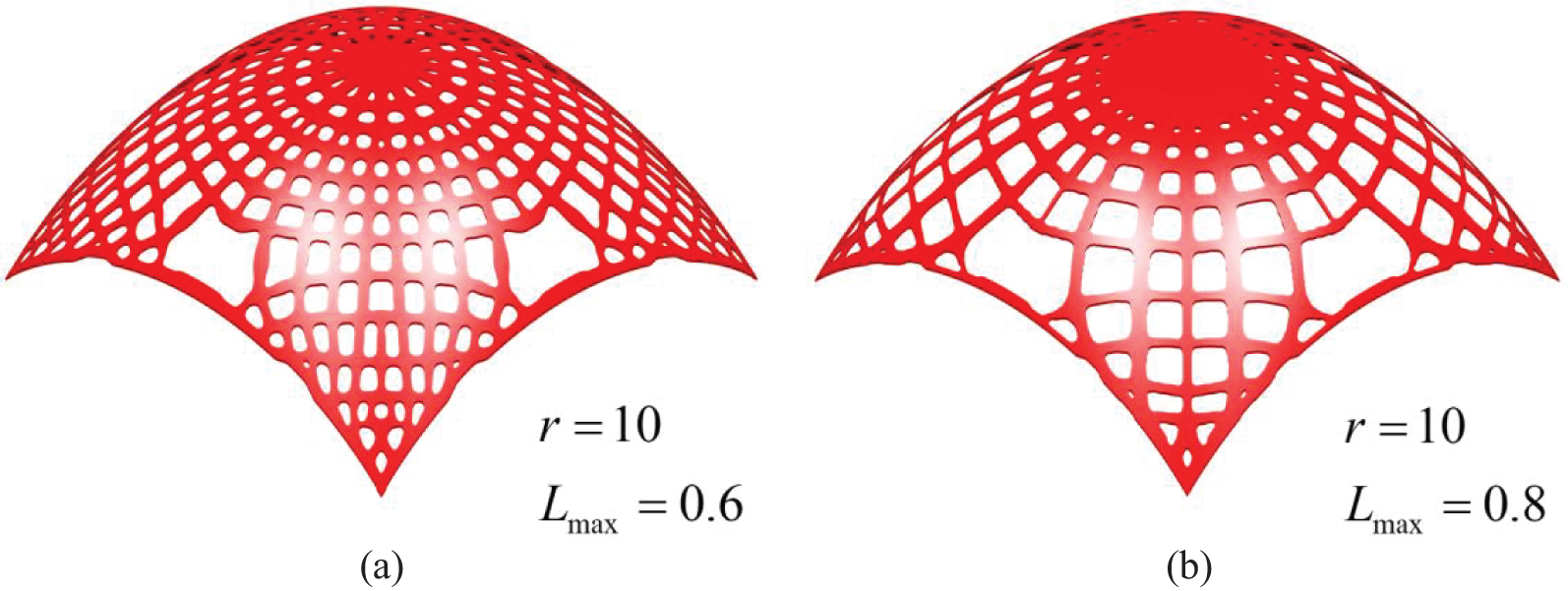
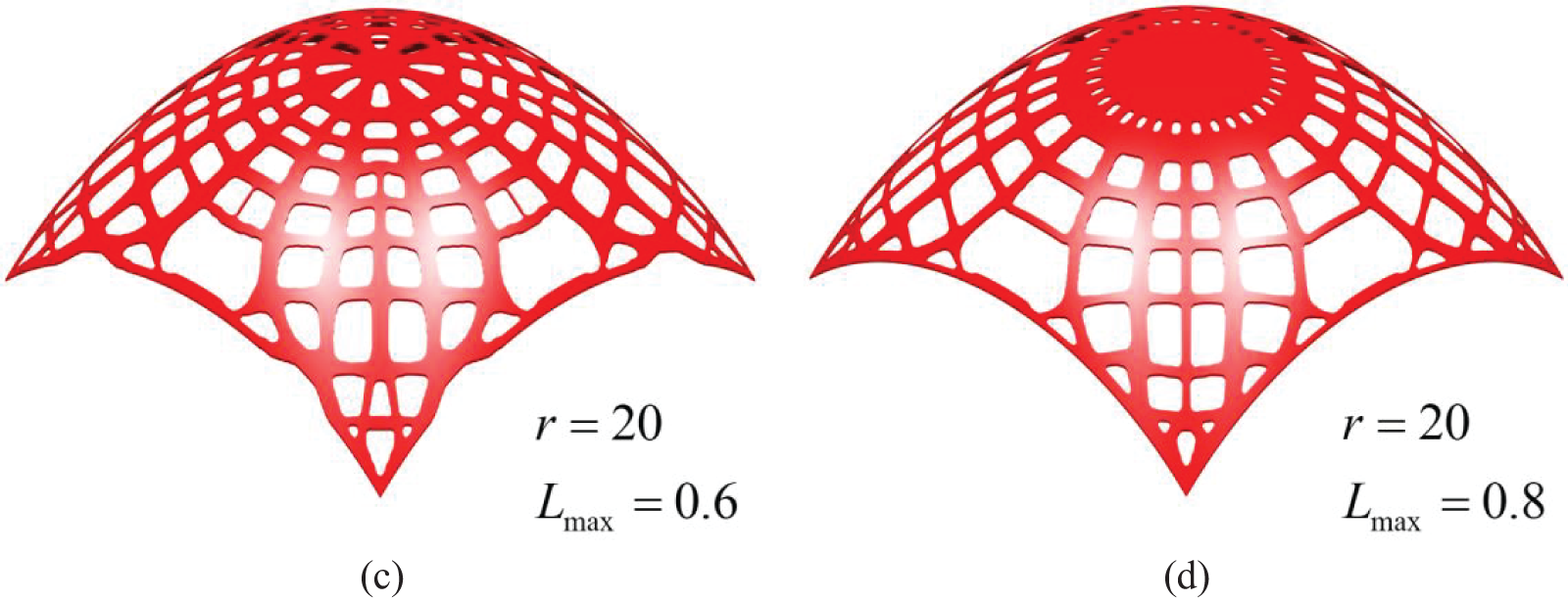
Figure 11: Optimized results of the blunt cone shell under different upper limits Lmax of the local volume constraint and influence radius r: (a) the optimized result under Lmax=0.6 and r=10; (b) the optimized result under Lmax=0.8 and r=10; (c) the optimized result under Lmax=0.6 and r=20; (d) the optimized result under Lmax=0.8 and r=20

4.3 Free-Form Surface

Fig. 12 shows the design domain of a free-form surface, where F1 = 50 N and F2 = 10 N. The design domain is discretized into 200 × 200 IGA elements, as displayed in Fig. 13. The thickness of the free-form surface is 1 mm. The parameters of the corresponding NURBS patch are provided in Table 3. The influence radius of the local volume fraction is set to 16.

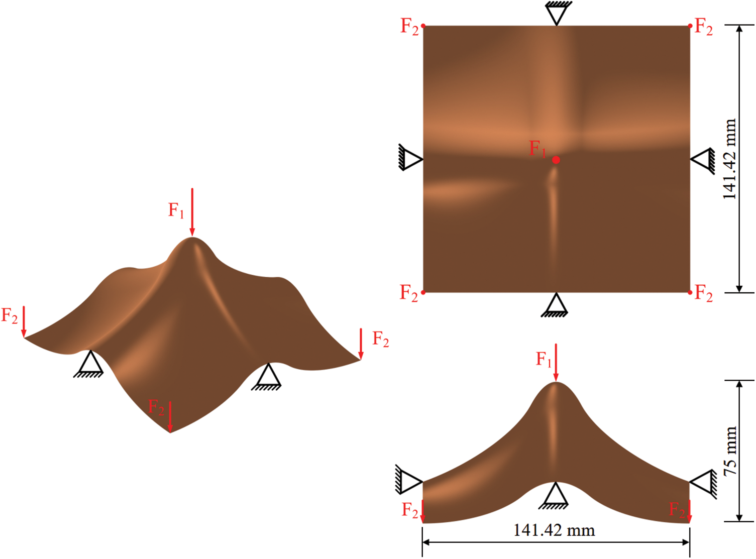
Figure 12: Design domain of the free-form surface

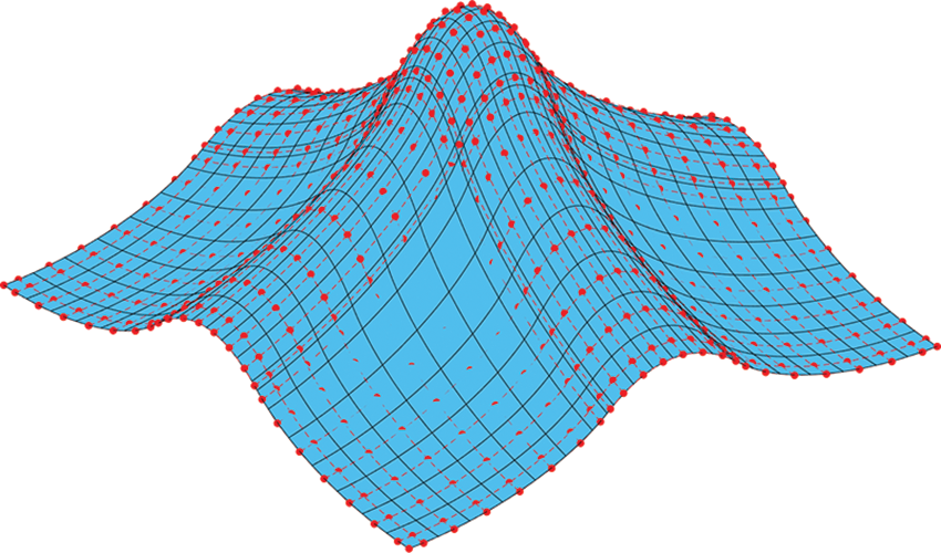
Figure 13: IGA mesh of the free-form surface, where the mesh resolution is set to one-tenth of the actual resolution for better visualization

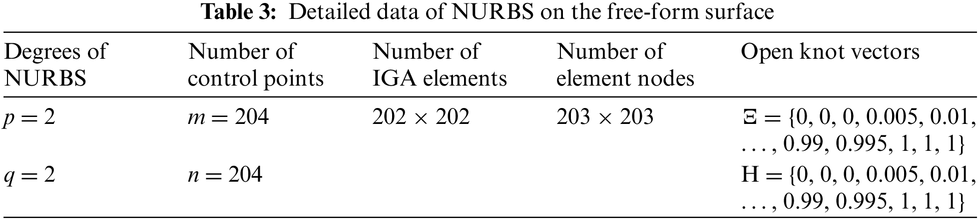
Fig. 14 depicts the iteration curves of the free-form surface. The iteration curves become stable after 200 iterations and the convergence condition is satisfied at the 653rd iteration step. Fig. 15 shows the optimized results obtained by the proposed method. A free-form surface with many holes is generated, and the material is mainly distributed along the main force transmission path. Fig. 16 shows the 3D-printed sample obtained by additive manufacturing for the optimized result of the free-form surface.

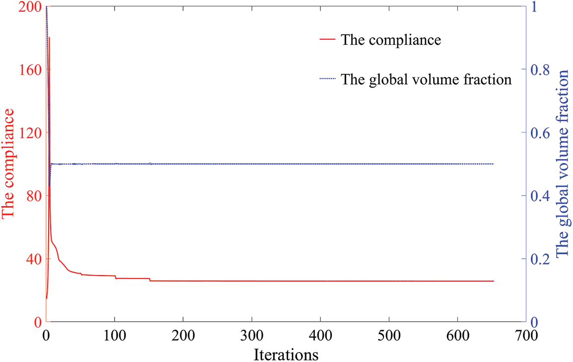
Figure 14: Iteration curves of the free-form surface

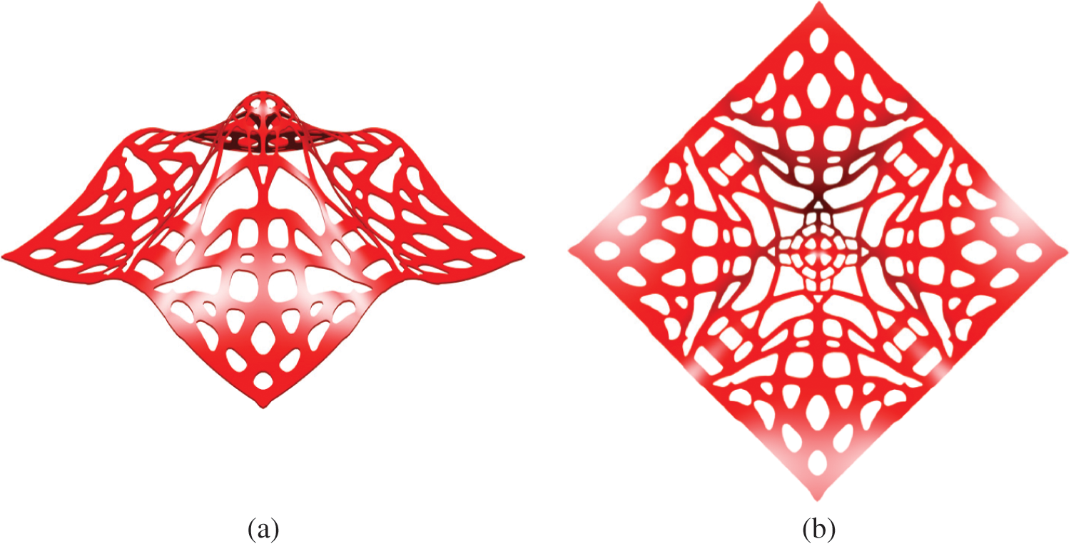
Figure 15: Optimized results of the free-form surface: (a) optimized cellular thin-shell structure; (b) top view of the cellular thin-shell structure

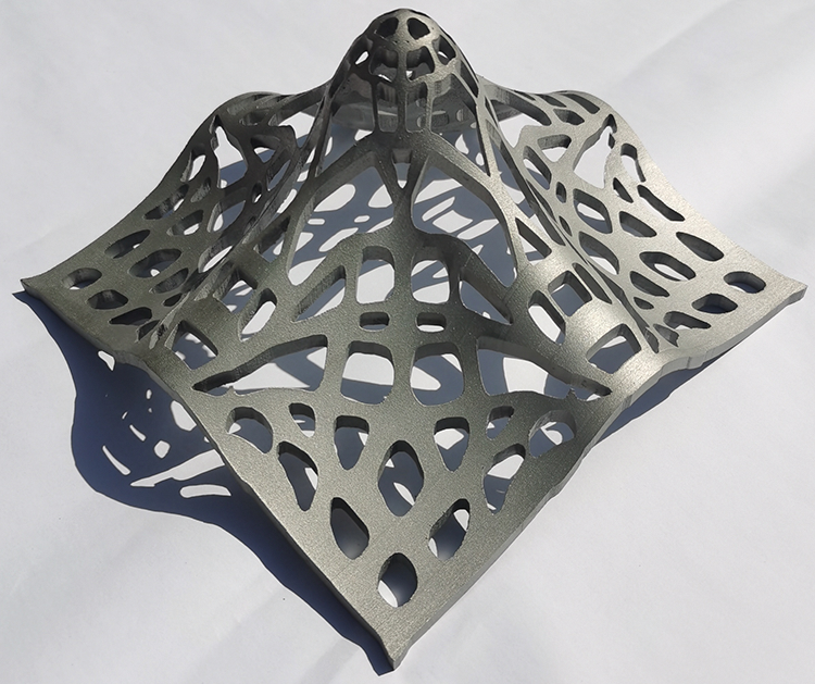
Figure 16: The 3D-printed sample of the optimized result of the free-form surface

In Fig. 17, the optimized structure obtained by the proposed method and the thin-shell structure with uniformly distributed holes are imported into COMSOL for simulation comparison. The same material properties and loading and boundary conditions are set in COMSOL. The optimized structure obtained by the proposed method has a 31.3% lower compliance and a 48.0% lower maximum displacement than the thin-shell structure with uniformly distributed holes. These results demonstrate that the proposed method can effectively improve the mechanical properties of thin-shell structures.

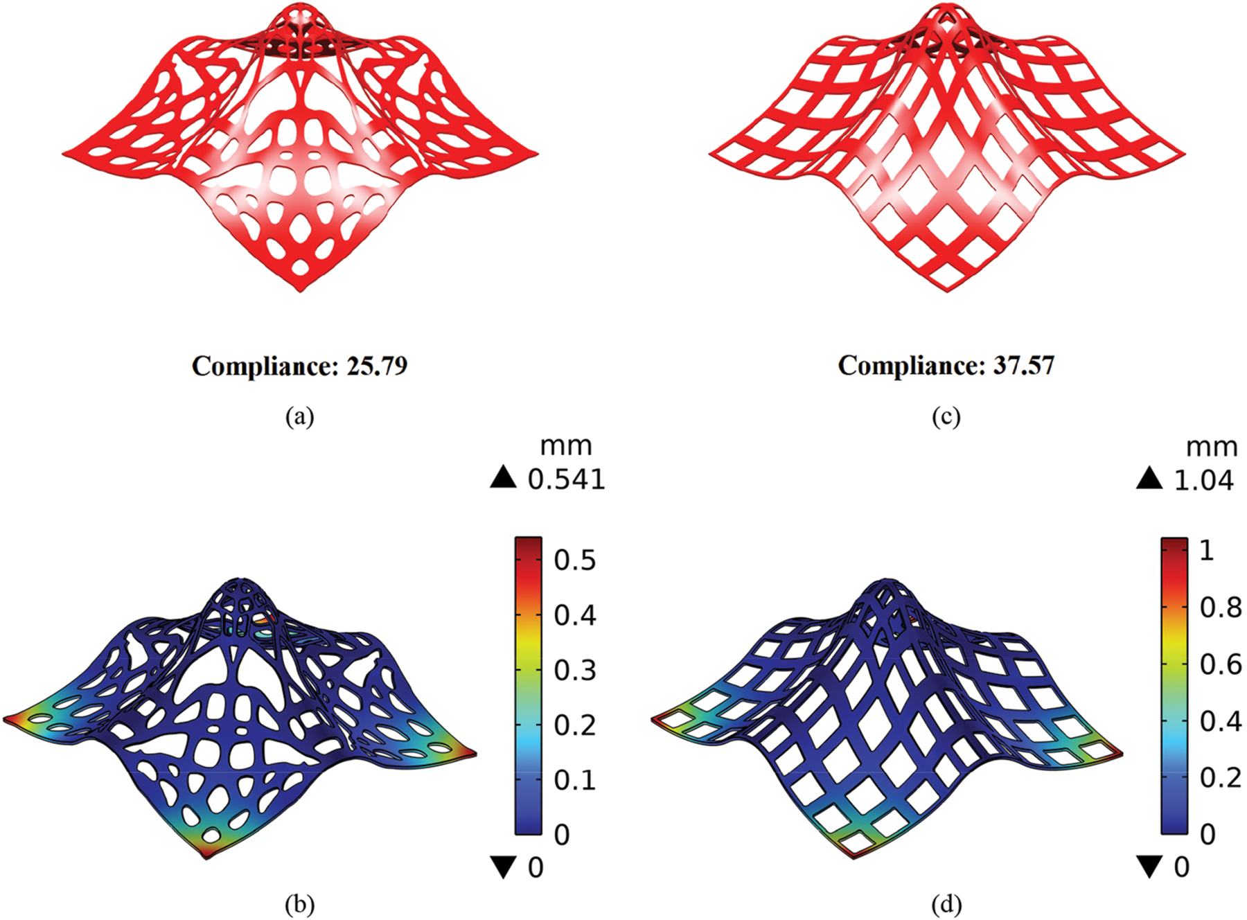
Figure 17: The free-form surfaces and corresponding displacement fields for (a) and (b): the proposed method, and (c) and (d): uniformly distributed holes

4.4 Cylindrical Shell

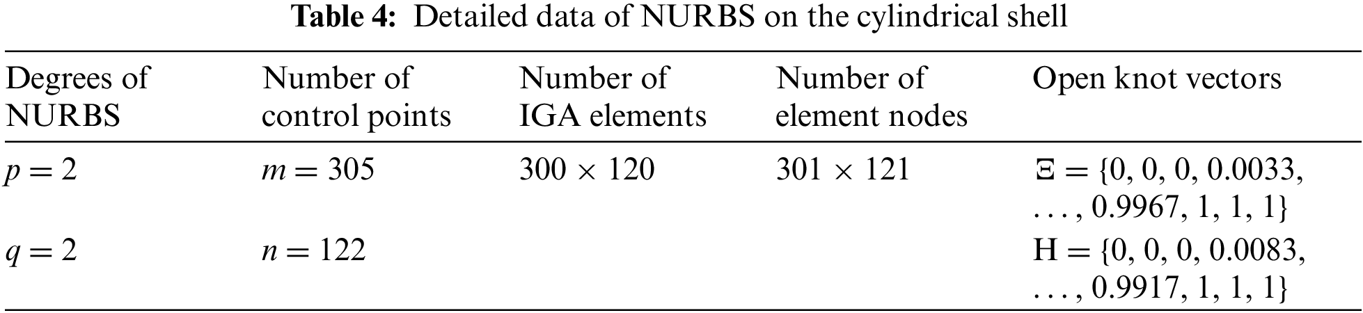
Fig. 18 displays a design domain of the thin cylindrical shell, where the tangential force F = 100 N. The thickness of the cylindrical shell is 1 mm. The design domain is meshed with 300 × 120 IGA elements, as shown in Fig. 19. The parameters of the corresponding IGA mesh are listed in Table 4. In the initial setting, the influence radius of the local volume fraction is set to 12.

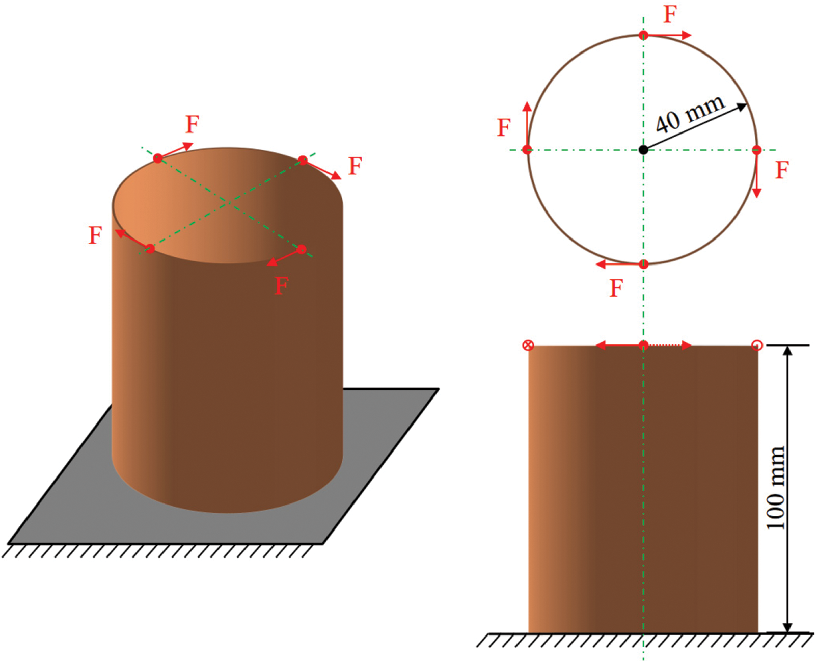
Figure 18: Design domain of the cylindrical shell

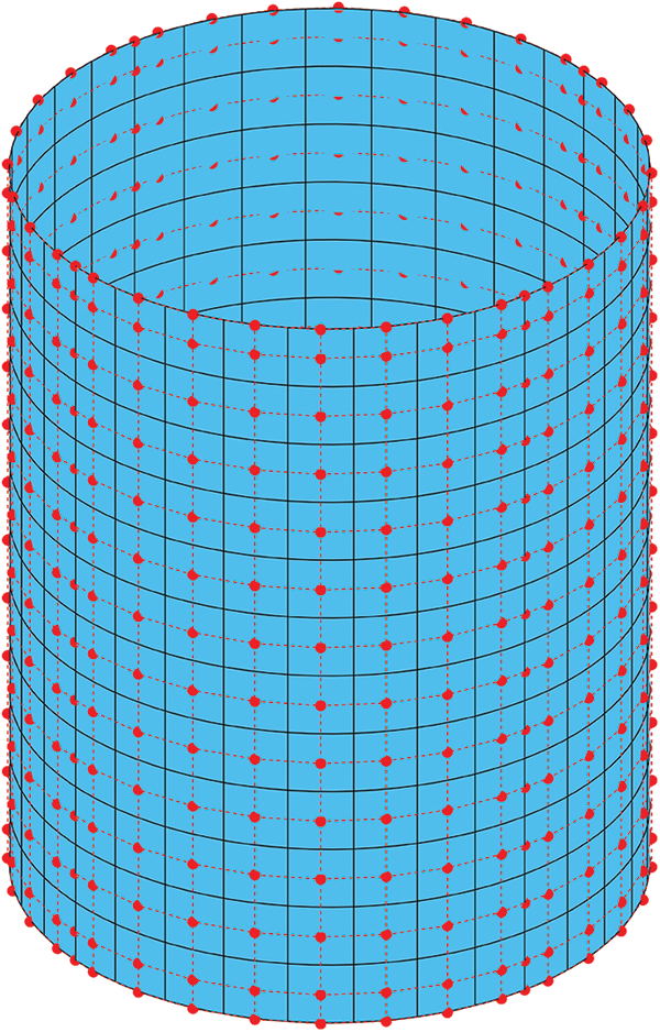
Figure 19: IGA mesh of the cylindrical shell, where the mesh resolution is set to one-tenth of the actual resolution for better visualization

The iteration curves of the cylindrical shell are shown in Fig. 20. Due to changes in σ, the iteration curves still exhibit slight oscillations in the first 200 iterations. Then, the iteration curves become stable and reach the minimum compliance at the 800th iteration step. Fig. 21 displays the optimized result of the cylindrical shell by the proposed method. The material is mainly distributed along the main force transmission path from the load application points at the top of the cylindrical shell to the fixed bottom. Since the applied forces are all tangential forces with the same magnitude and clockwise direction, the optimized structure is highly symmetrical. Meanwhile, many bone-like cellular structures are present in the cylindrical shell due to the influence of local volume constraints. Fig. 22 shows the 3D-printed sample obtained by additive manufacturing for the optimized result of the cylindrical shell.

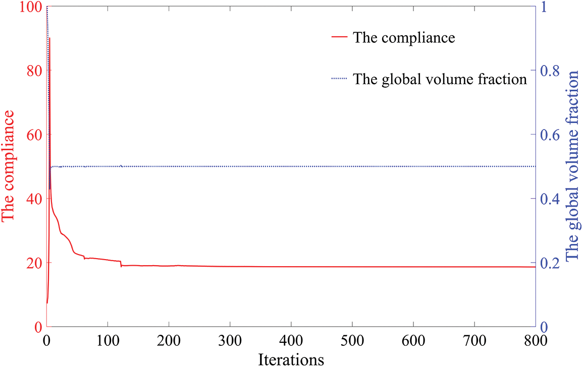
Figure 20: Iteration curves of the cylindrical shell

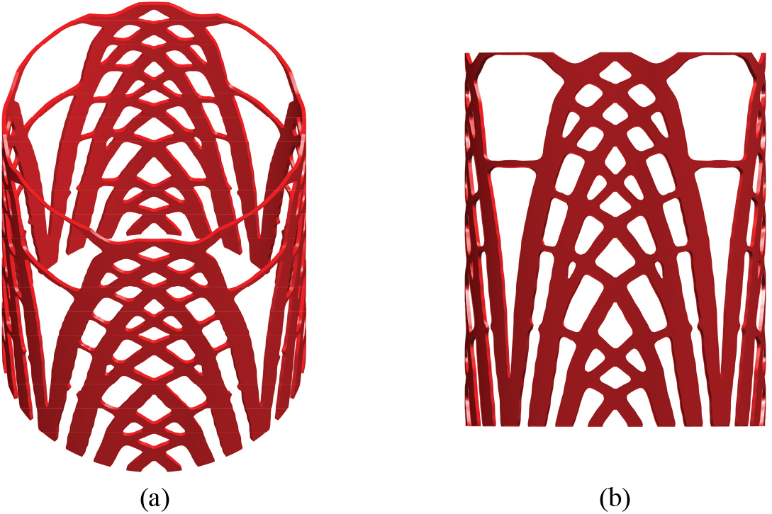
Figure 21: Optimized results of the cylindrical shell: (a) optimized cellular thin-shell structure; (b) elevation view of the cellular thin-shell structure

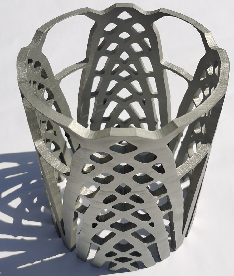
Figure 22: The 3D-printed sample of the optimized result of the cylindrical shell

A major advantage of the cellular thin-shell structure optimized by the proposed method is its excellent damage tolerance ability. Even if the structure is damaged to a certain extent, the performance of the structure will not be greatly impacted. Figs. 23a and 23b show the optimized results by the proposed method and classical topology optimization, respectively. Unlike the proposed method, the classical topology optimization method does not set local volume constraints. The material in the blue area is removed to simulate local failure. Comparing the compliances of the two structures before and after local failure reveals that before the local failure, the compliance of the optimized structure obtained by the proposed method is 20.3% greater than that by the classical topology optimization; however, after the local failure, the compliance of the optimized structure obtained by the proposed method is 39.4% less than that by the classical topology optimization. In addition, the compliance of the optimized structure obtained by the proposed method is 21.2% greater after local failure, while the compliance of that by the classical topology optimization is 140.6% greater. These results demonstrate that local failure has less influence on the mechanical properties of the structure optimized by the proposed method than on the structure optimized by classical topology optimization.

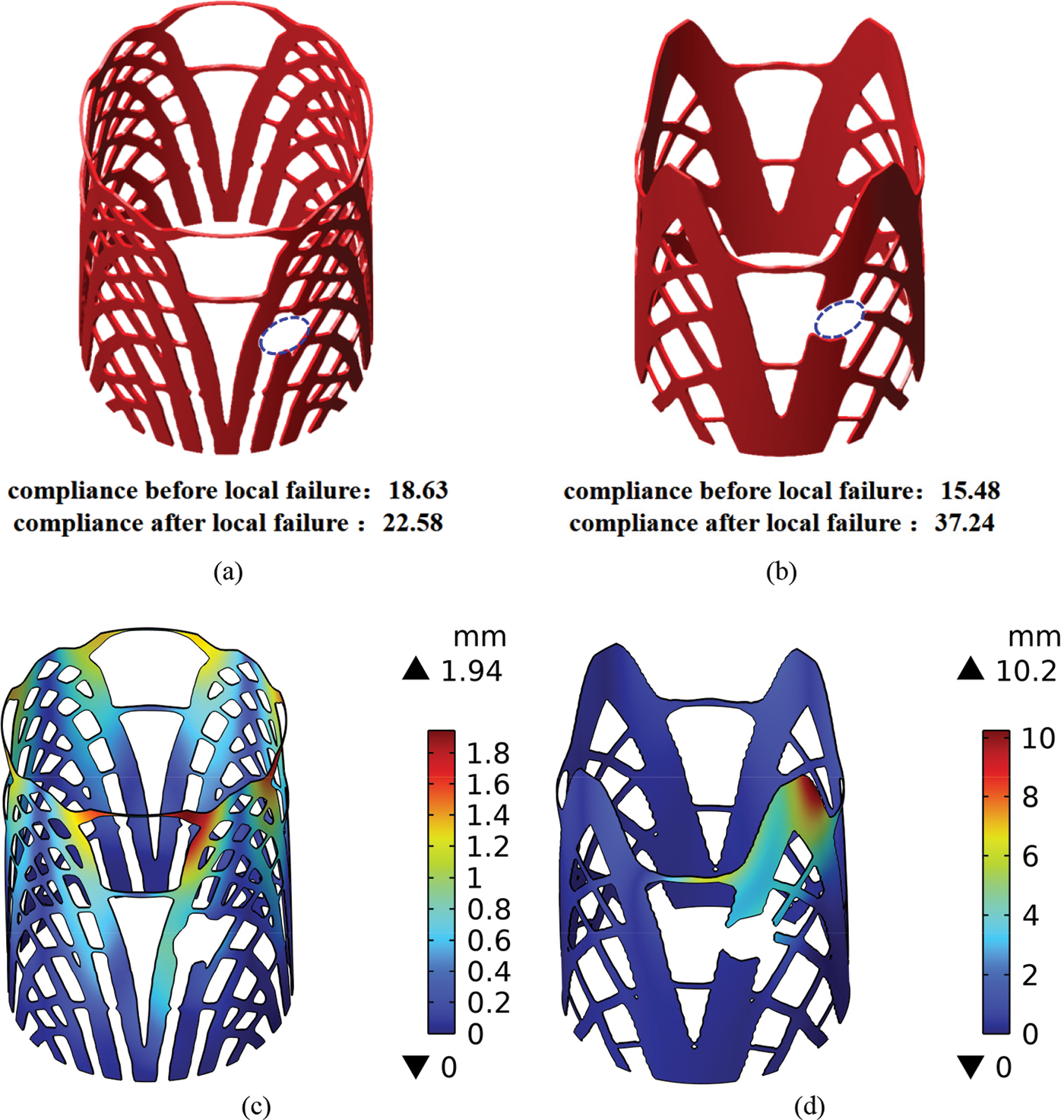
Figure 23: Optimized results of the cylindrical shell after local failure: (a) and (b) the optimized results by the proposed method and classical topology optimization after local failure; (c) and (d) displacement fields of optimized results by the proposed method and classical topology optimization after local failure

The two structures after local failure are then imported into COMSOL for simulation. The same material properties and loading and boundary conditions are applied in COMSOL. The displacement fields of the two structures are shown in Figs. 23c and 23d. The maximum displacement of the optimized structure obtained by the proposed method is 80.1% smaller than the maximum displacement of that by the classical topology optimization. Therefore, the cellular thin-shell structure optimized by the proposed method has excellent robustness to local failure.

5  Conclusions

This paper presents a full-scale ITO method to realize the design of cellular thin-shell structures with excellent bearing capacity and damage tolerance. High-order continuous NURBS is adopted to build the geometric and Kirchhoff–Love models of thin shells. The displacement field of a thin-shell structure is computed by IGA with high computational accuracy. A full-scale ITO framework is established by introducing local volume constraints, which can generate bone-like structures on thin shells. The size of the holes in the cellular thin-shell structures can be adjusted by changing the local volume constraints and their influence on radii. Local volume constraints are aggregated by the p-norm function to facilitate an effective optimization process. The effectiveness of the proposed method is verified by several numerical examples. These numerical examples show that the proposed full-scale ITO method can steadily generate cellular structures in various irregular design domains of thin shells. The comparative discussion demonstrates that the optimized structure obtained by the proposed method has high bearing capacity and great robustness to local damage, enabling its use in practical engineering applications with high requirements for safety factors.

However, importantly, the optimized results obtained by the proposed method may have buckling or stress constraint problems due to the presence of overly thin substructures. To address these issues, future work will consider incorporating buckling and stress constraints into the optimization process to optimize the mechanical properties of cellular thin-shell structures more comprehensively.

Acknowledgement: Thanks to the help of three anonymous reviewers and journal editors, the logical organization and content quality of this paper have been improved.

Funding Statement: This research was supported by the National Key R&D Program of China (Grant Number 2020YFB1708300), China National Postdoctoral Program for Innovative Talents (Grant Number BX20220124), China Postdoctoral Science Foundation (Grant Number 2022M710055), the New Cornerstone Science Foundation through the XPLORER PRIZE, the Knowledge Innovation Program of Wuhan-Shuguang, the Young Top-Notch Talent Cultivation Program of Hubei Province and the Taihu Lake Innovation Fund for Future Technology (Grant Number HUST: 2023-B-7).

Author Contributions: The authors confirm contribution to the paper as follows: study conception and design: Mingzhe Huang, Mi Xiao, Liang Gao; data collection: Mingzhe Huang, Mian Zhou; analysis and interpretation of results: Wei Sha, Jinhao Zhang; draft manuscript preparation: Mingzhe Huang, Mi Xiao. All authors reviewed the results and approved the final version of the manuscript.

Availability of Data and Materials: The data and models generated and optimized in this paper are available from the corresponding author on reasonable request.

Conflicts of Interest: The authors declare that they have no conflicts of interest to report regarding the present study.

References

1. Suarez Espinoza, P. A., Bletzinger, K., Hörnlein, H. R. E. M., Daoud, F., Schuhmacher, G. et al. (2012). Shape optimisation in the design of thin-walled shells as components of aerospace structures. The Aeronautical Journal, 116(1182), 793–814. [Google Scholar]

2. Lee, H., Seo, H., Park, G. (2003). Design enhancements for stress relaxation in automotive multi-shell-structures. International Journal of Solids and Structures, 40(20), 5319–5334. [Google Scholar]

3. Zingoni, A. (2015). Liquid-containment shells of revolution: A review of recent studies on strength, stability and dynamics. Thin-Walled Structures, 87, 102–114. [Google Scholar]

4. Benson, D. J., Bazilevs, Y., Hsu, M. C., Hughes, T. J. R. (2009). Isogeometric shell analysis: The Reissner-Mindlin shell. Computer Methods in Applied Mechanics and Engineering, 199(5), 276–289. [Google Scholar]

5. Kiendl, J., Bazilevs, Y., Hsu, M. C., Wüchner, R., Bletzinger, K. U. (2010). The bending strip method for isogeometric analysis of Kirchhoff-Love shell structures comprised of multiple patches. Computer Methods in Applied Mechanics and Engineering, 199(37), 2403–2416. [Google Scholar]

6. Chapelle, D., Bathe, K. J. (1998). Fundamental considerations for the finite element analysis of shell structures. Computers and Structures, 66(1), 19–36. [Google Scholar]

7. Hughes, T. J. R., Cottrell, J. A., Bazilevs, Y. (2005). Isogeometric analysis: CAD, finite elements, NURBS, exact geometry and mesh refinement. Computer Methods in Applied Mechanics and Engineering, 194(39–41), 4135–4195. [Google Scholar]

8. Cottrell, J. A., Hughes, T. J. R., Bazilevs, Y. (2009). Isogeometric analysis: Toward integration of CAD and FEA. UK: John Wiley & Sons. [Google Scholar]

9. Kiendl, J., Bletzinger, K. U., Linhard, J., Wüchner, R. (2009). Isogeometric shell analysis with Kirchhoff-Love elements. Computer Methods in Applied Mechanics and Engineering, 198(49–52), 3902–3914. [Google Scholar]

10. Guo, Y., Ruess, M. (2015). Nitsche's method for a coupling of isogeometric thin shells and blended shell structures. Computer Methods in Applied Mechanics and Engineering, 284, 881–905. [Google Scholar]

11. Li, W., Nguyen-Thanh, N., Zhou, K. (2018). Geometrically nonlinear analysis of thin-shell structures based on an isogeometric-meshfree coupling approach. Computer Methods in Applied Mechanics and Engineering, 336, 111–134. [Google Scholar]

12. Nguyen-Thanh, N., Li, W., Zhou, K. (2018). Static and free-vibration analyses of cracks in thin-shell structures based on an isogeometric-meshfree coupling approach. Computational Mechanics, 62, 1287–1309. [Google Scholar]

13. Zhang, Q., Nguyen-Thanh, N., Li, W., Zhang, A., Li, S. et al. (2023). A coupling approach of the isogeometric-meshfree method and peridynamics for static and dynamic crack propagation. Computer Methods in Applied Mechanics and Engineering, 410, 115904. [Google Scholar]

14. Hirschler, T., Bouclier, R., Dureisseix, D., Duval, A., Elguedj, T. et al. (2019). A dual domain decomposition algorithm for the analysis of non-conforming isogeometric Kirchhoff-Love shells. Computer Methods in Applied Mechanics and Engineering, 357, 112578. [Google Scholar]

15. Zareh, M., Qian, X. (2019). Kirchhoff-Love shell formulation based on triangular isogeometric analysis. Computer Methods in Applied Mechanics and Engineering, 347, 853–873. [Google Scholar]

16. Miao, D., Zou, Z., Scott, M. A., Borden, M. J., Thomas, D. C. (2021). Isogeometric Bézier dual mortaring: The Kirchhoff-Love shell problem. Computer Methods in Applied Mechanics and Engineering, 382, 113873. [Google Scholar]

17. Peng, X., Zheng, C. (2022). An isogeometric cloth simulation based on fast projection method. Computer Modeling in Engineering & Sciences, 134(3), 1837–1853. https://doi.org/10.32604/cmes.2022.022367 [Google Scholar] [CrossRef]

18. Maurin, F., Greco, F., Desmet, W. (2019). Isogeometric analysis for nonlinear planar pantographic lattice: Discrete and continuum models. Continuum Mechanics and Thermodynamics, 31, 1051–1064. [Google Scholar]

19. Kiendl, J., Hsu, M., Wu, M. C. H., Reali, A. (2015). Isogeometric Kirchhoff-Love shell formulations for general hyperelastic materials. Computer Methods in Applied Mechanics and Engineering, 291, 280–303. [Google Scholar]

20. Tepole, A. B., Kabaria, H., Bletzinger, K., Kuhl, E. (2015). Isogeometric Kirchhoff-Love shell formulations for biological membranes. Computer Methods in Applied Mechanics and Engineering, 293, 328–347. [Google Scholar] [PubMed]

21. Xiao, X., Sabin, M., Cirak, F. (2019). Interrogation of spline surfaces with application to isogeometric design and analysis of lattice-skin structures. Computer Methods in Applied Mechanics and Engineering, 351, 928–950. [Google Scholar]

22. Sun, Y., Zhou, Y., Ke, Z., Tian, K., Wang, B. (2022). Stiffener layout optimization framework by isogeometric analysis-based stiffness spreading method. Computer Methods in Applied Mechanics and Engineering, 390, 114348. [Google Scholar]

23. Andreassen, E., Clausen, A., Schevenels, M., Lazarov, B. S., Sigmund, O. (2011). Efficient topology optimization in MATLAB using 88 lines of code. Structural and Multidisciplinary Optimization, 43(1), 1–16. [Google Scholar]

24. Wang, Y., Li, X., Long, K., Wei, P. (2023). Open-source codes of topology optimization: A summary for beginners to start their research. Computer Modeling in Engineering & Sciences, 137(1), 1–34. https://doi.org/10.32604/cmes.2023.027603 [Google Scholar] [CrossRef]

25. Hassani, B., Khanzadi, M., Tavakkoli, S. M. (2012). An isogeometrical approach to structural topology optimization by optimality criteria. Structural and Multidisciplinary Optimization, 45(2), 223–233. [Google Scholar]

26. Wang, Y., Benson, D. J. (2016). Isogeometric analysis for parameterized LSM-based structural topology optimization. Computational Mechanics, 57(1), 19–35. [Google Scholar]

27. Gao, J., Gao, L., Luo, Z., Li, P. (2019). Isogeometric topology optimization for continuum structures using density distribution function. International Journal for Numerical Methods in Engineering, 119(10), 991–1017. [Google Scholar]

28. Zhu, H., Gao, X., Yang, A., Wang, S., Xie, X. et al. (2022). Explicit isogeometric topology optimization method with suitably graded truncated hierarchical B-spline. Computer Modeling in Engineering & Sciences, 135(2), 1435–1456. https://doi.org/10.32604/cmes.2022.023454 [Google Scholar] [CrossRef]

29. Kang, P., Youn, S. (2016). Isogeometric topology optimization of shell structures using trimmed NURBS surfaces. Finite Elements in Analysis & Design, 120, 18–40. [Google Scholar]

30. Zhang, W., Jiang, S., Liu, C., Li, D., Kang, P. et al. (2020). Stress-related topology optimization of shell structures using IGA/TSA-based Moving Morphable Void (MMV) approach. Computer Methods in Applied Mechanics and Engineering, 366, 113036. [Google Scholar]

31. Zhang, Y., Xiao, M., Gao, L., Gao, J., Li, H. (2020). Multiscale topology optimization for minimizing frequency responses of cellular composites with connectable graded microstructures. Mechanical Systems and Signal Processing, 135, 106369. [Google Scholar]

32. Xiao, M., Liu, X., Zhang, Y., Gao, L., Gao, J. et al. (2021). Design of graded lattice sandwich structures by multiscale topology optimization. Computer Methods in Applied Mechanics and Engineering, 384, 113949. [Google Scholar]

33. Liu, X., Gao, L., Xiao, M., Zhang, Y. (2022). Kriging-assisted design of functionally graded cellular structures with smoothly-varying lattice unit cells. Computer Methods in Applied Mechanics and Engineering, 390, 114466. [Google Scholar]

34. Ali, M. A., Shimoda, M. (2022). Investigation of concurrent multiscale topology optimization for designing lightweight macrostructure with high thermal conductivity. International Journal of Thermal Sciences, 179, 107653. [Google Scholar]

35. Wu, J., Sigmund, O., Groen, J. P. (2021). Topology optimization of multi-scale structures: A review. Structural and Multidisciplinary Optimization, 63(3), 1455–1480. [Google Scholar]

36. Xu, M., Xia, L., Wang, S., Liu, L., Xie, X. (2019). An isogeometric approach to topology optimization of spatially graded hierarchical structures. Composite Structures, 225, 111171. [Google Scholar]

37. Wu, J., Aage, N., Westermann, R., Sigmund, O. (2017). Infill optimization for additive manufacturing—Approaching bone-like porous structures. IEEE Transactions on Visualization and Computer Graphics, 24(2), 1127–1140. [Google Scholar] [PubMed]

38. Wang, F., Lazarov, B. S., Sigmund, O. (2011). On projection methods, convergence and robust formulations in topology optimization. Structural and Multidisciplinary Optimization, 43(6), 767–784. [Google Scholar]

39. Cirak, F., Scott, M. J., Antonsson, E. K., Ortiz, M., Schröder, P. (2002). Integrated modeling, finite-element analysis, and engineering design for thin-shell structures using subdivision. Computer-Aided Design, 34(2), 137–148. [Google Scholar]

40. Bandara, K., Cirak, F. (2018). Isogeometric shape optimisation of shell structures using multiresolution subdivision surfaces. Computer-Aided Design, 95, 62–71. [Google Scholar]

41. Aage, N., Lazarov, B. S. (2013). Parallel framework for topology optimization using the method of moving asymptotes. Structural and Multidisciplinary Optimization, 47(4), 493–505. [Google Scholar]

42. Macneal, R. H., Harder, R. L. (1985). A proposed standard set of problems to test finite element accuracy. Finite Elements in Analysis and Design, 1(1), 3–20. [Google Scholar]