PCA-LSTM: An Impulsive Ground-Shaking Identification Method Based on Combined Deep Learning

1  Introduction

In recent times, several studies have shown that impulsive ground-shaking has a particularly destructive effect on buildings and structures [1–4]. It is more likely to result in high-impact forces and deformations in engineering structures during near-fault ground-shaking compared to other types of ground-shaking. For example, significant damage due to impulsive ground-shaking was observed after the Northridge earthquake in 1994 [5], the Kobe earthquake in 1995 [6], the Chi-Chi earthquake in 1999 [7], and the Wenchuan earthquake in 2008 [8]. Therefore, (i) early warning and assessment of ground-shaking hazards to engineering structures, (ii) in-depth exploration of the generation mechanism and propagation law of impulsive ground-shaking, and (iii) the establishment of accurate and reliable identification models, are the most urgent issues in seismological research at present.

Numerous studies have proposed a series of different identification methods for impulsive ground-shaking, which essentially solve the problems due to manual subjective identification. Baker et al. [9] proposed and improved a quantitative method based on wavelet analysis for reproducible identification of impulsive ground-shaking recordings. It adopts a fourth-order Daubechies wavelet basis, extracts the maximum velocity pulse during the ground-shaking time course using wavelet decomposition, and gives quantitative discrimination criteria for the pulse by analyzing the energy and peak velocity ratio between the residual and original records. Chang et al. [10] proposed a method that relies on the pulse amplitude, pulse period, number of half-cyclic pulses, and phase to capture the main features of the velocity pulse. This method extracts the velocity pulse through the pulse model and then identifies it quantitatively based on the relative energy index. Zhao et al. [11] used trigonometric functions and proposed a quantitative identification method that uses the value of the detected pulse energy with respect to the original ground-shaking energy as a discriminant criterion, and refined the single- and multi-pulse identification methods. However, due to the strong nonlinear characteristics and complexity of the ground-shaking data, manual analysis may be required for specific cases as the established models may not be suitable due to poor generality. Moreover, the complexity of the models built by the traditional methods slows down the ground-shaking analysis. Therefore, novel impulsive ground-shaking identification methods are required to simplify the model and make it more universal.

With the rapid development of key technologies in the field of computing, deep learning (DL), an important branch of artificial intelligence, originated from the research and development of Artificial Neural Network (ANN) [12]. Unlike the traditional “shallow learning” methods, such as support vector machines, boosting, and maximum entropy, DL models possess a deeper structure, usually with non-linear operations occurring at the hidden layer levels, and enhanced feature learning and expressive capabilities. Instead of depending on manual experience to extract sample features, these models automatically learn to achieve hierarchical feature representations by performing layer-by-layer feature transformations on raw data [13]. The core of DL lies in efficiently selecting valuable features by constructing hierarchical neural network (NN) models with vast amounts of training data.

In recent years, DL has become an effective mathematical analysis tool, gradually applied to various types of geophysical studies [14–17]. Zhang et al. [18] applied Convolutional Neural Network (CNN) to realize the classification of microseismic waveforms, combined with wavelet transform for decomposing the frequency spectrum into a time-frequency spectrum and distinguished between seismic signals and interference noises. Chen et al. [19] combined the K-averaging algorithm and CNN (K-CNN) to accurately classify seismic waveforms by training the model on synthetic and field microseismic data with varying noise levels. Ku et al. [20] developed an attention-based feature aggregation framework embedded in a multitasking learning architecture for accurate earthquake event type classification. In summary, although DL has been widely used in seismic fields, there is a lack of methods for impulsive ground-shaking identification.

Compared to other DL methods, the Long Short-Term Memory network (LSTM) [21] offers the advantages of robust data processing capabilities and simplicity, which make it a highly feasible method for impulsive ground-shaking identification. However, earthquakes produce a large number of complex feature data, which contain redundant ground-shaking features. If not processed properly, these features will inevitably lead to computational inefficiency and wastage of resources, which will negatively impact the subsequent prediction results [22]. This study addressed the aforementioned issues through (1) comprehensively analyzing the impulsive ground-shaking features and performing preliminary feature screening; (2) extracting features directly related to impulsive ground-shaking by Principal Component Analysis (PCA), removing redundant feature data, and obtaining more value with fewer data points; and (3) establishing a PCA-LSTM model by combining with ANN to accurately and efficiently identify impulsive ground-shaking.

The remainder of this paper is organized as follows: Section 2 presents the theory of impulsive ground-shaking and the identification method. Section 3 presents the analysis of the training and evaluation of the impulsive ground-shaking identification model. Section 4 provides the conclusions of the study. Finally, Section 5 focuses on the possible improvements to the model in future works.

2  Theory and Methods

As shown in Fig. 1, the overall framework of the impulsive ground-shaking identification method consists of three main components: 1) pre-processing of ground-shaking data; 2) ground-shaking feature extraction; and 3) training and evaluation of the impulsive ground-shaking identification model.

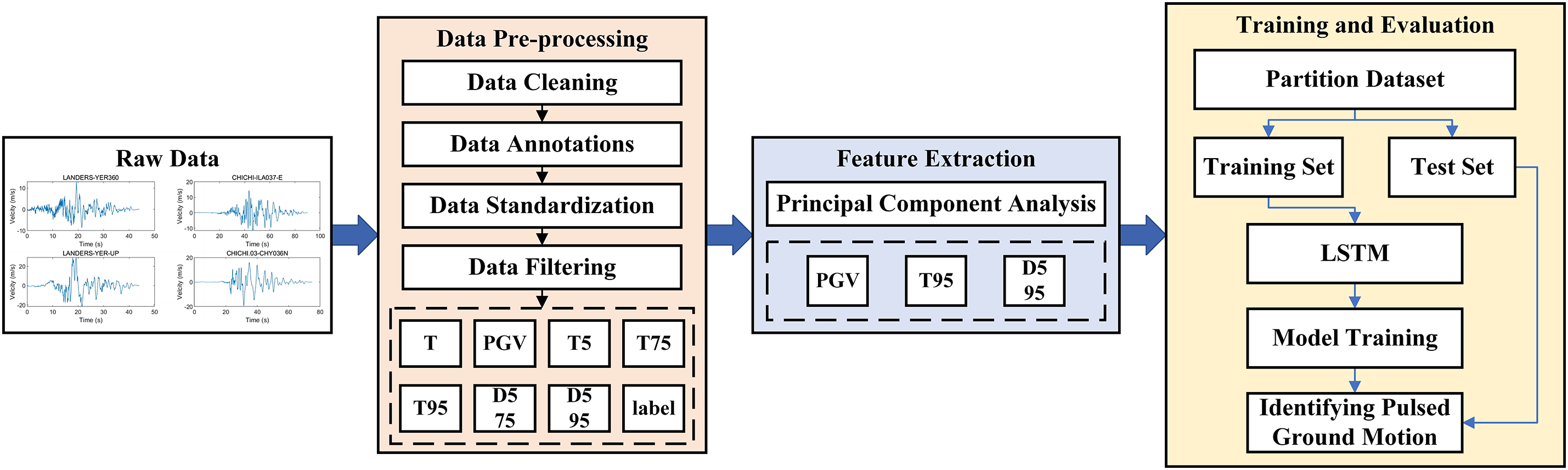
Figure 1: The overall framework of the impulsive ground-shaking identification method

2.1 Pre-Processing of Ground Shaking Data

2.1.1 Overview of the Chi-Chi Earthquake

The ground-shaking data used in this paper was obtained from the earthquake database provided by the United States Geological Survey (USGS). The Chi-Chi earthquake of 1999 [23] was the largest earthquake of its magnitude to have occurred on the Taiwanese islands. This event has been of great significance in earthquake research [24–26]. The extent of its impact and damages observed by seismic stations is illustrated in Fig. 2. This earthquake resulted in substantial damage and casualties, exerting a profound socio-economic impact on Taiwan. Official statistics reported 2,470 fatalities, 11,305 injuries, damage to over 100,000 structures, including the collapse of several bridges and dams, and economic losses totaling approximately US$ 9.2 B. Due to the evident impulsive ground-shaking characteristics and its severe impact on engineering structures, the data from the Chi-Chi earthquake was selected for this study. The ground-shaking dataset was obtained from 421 seismic stations observing the earthquake, which contained a total of 592 ground-shaking datasets including ground-shaking velocity and acceleration information (Fig. 3).

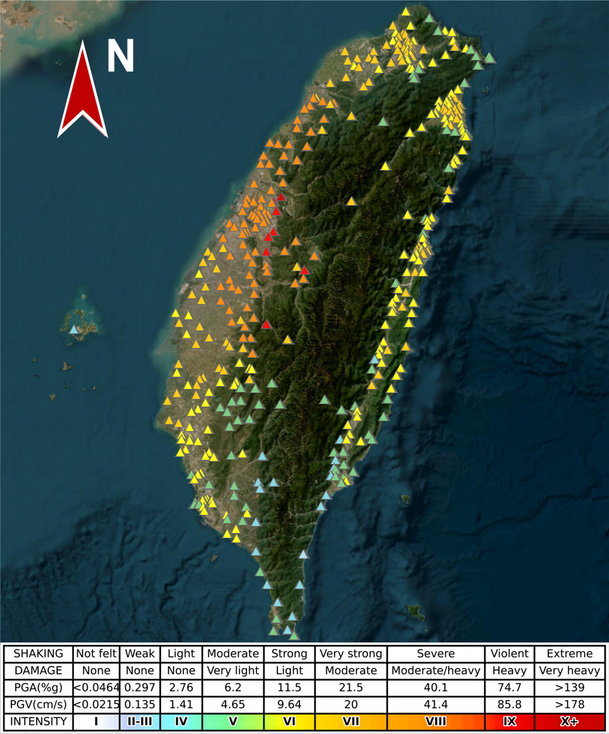
Figure 2: Taiwan Chi-Chi earthquake impact distribution (1999)

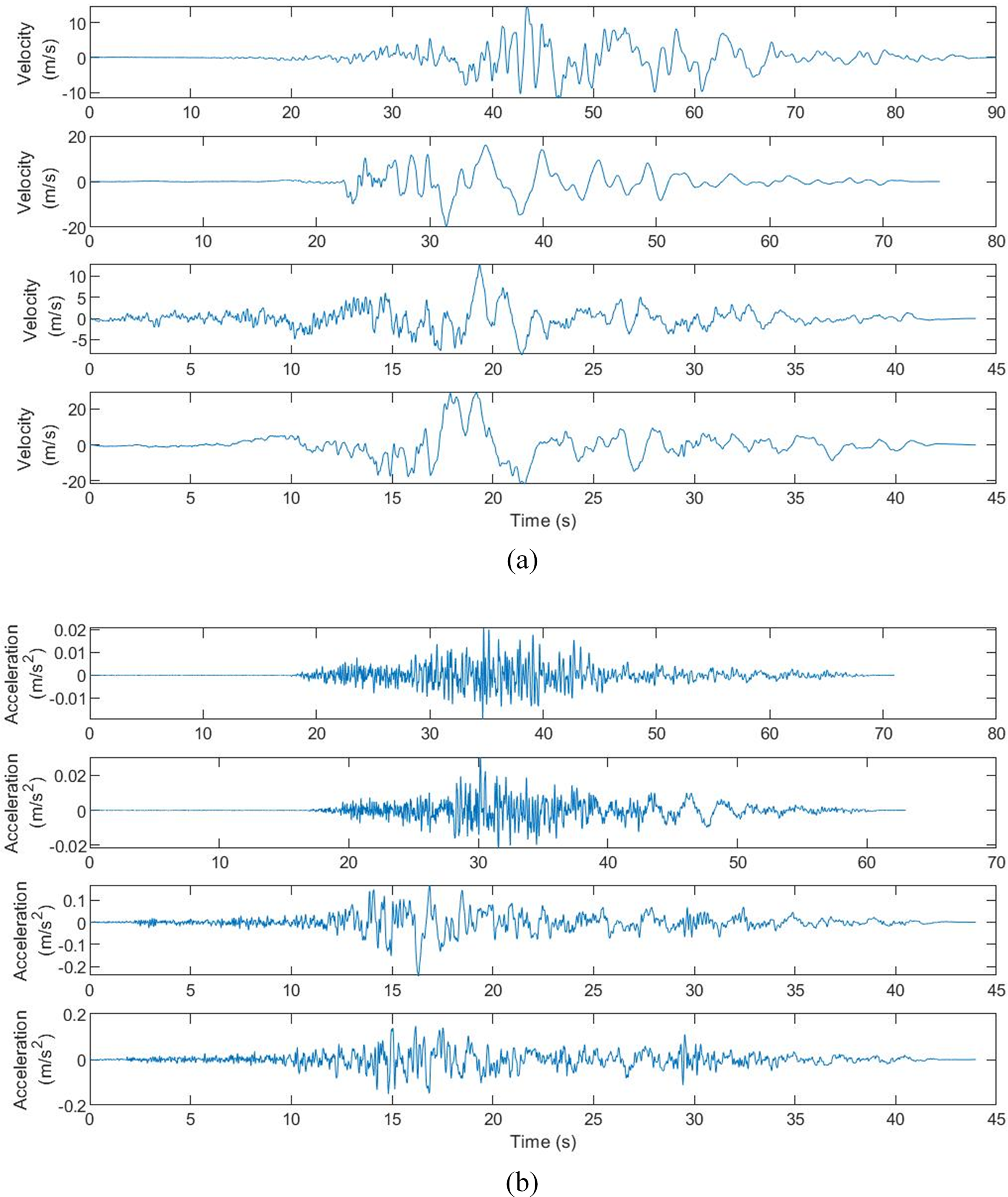
Figure 3: Examples of ground-shaking (a) velocity and (b) acceleration information from the raw data

The velocity impulse ground-shaking data is often characterized by large amplitudes, long characteristic periods, large instantaneous cumulative energies, and strong non-stationarity [27,28]. The amplitude and period of the ground-shaking velocity impulse are two main parameters to control the structure deformation. These parameters can reflect the intensity and frequency characteristics of impulsive ground-shaking, which impact the degree of damage to the engineering structures [29,30]. Therefore, considering the feasibility of verifying the velocity shock characteristics in existing studies and the convenience of practical measurements, the seismic wave velocity characteristics were selected to accurately assess the damage of shocks to structures as the criterion for impulsive ground-shaking identification.

After the screening, the acceleration data was removed from the dataset and all the subsequent studies were based on the remaining ground-shaking velocity datasets (a total of 356 data points).

2.1.2 Labeling of Raw Data

The velocity impulse type ground-shaking usually has the following characteristics: 1) energy concentration: releases a large amount of energy in a short period of time; 2) sudden and unpredictable increase/decrease in a short period of time; and 3) large peak velocity to peak acceleration ratio. These velocity impulse characteristics were combined with a widely used energy-based pulse identification method. The velocity and acceleration information in the raw data for labeling are shown in Fig. 3. In the original dataset, when the ground-shaking data meets the following conditions, it is characterized as impulsive ground-shaking.

In the raw data,

1) Peak ground velocity: PGV>30 cm/s

2) Pulse indicator: PI>0.85, which can be expressed as Eq. (1).

PI=11+e−23.3+14.6PGVratio+20.5Eratio,(1)

where PGVratio is the ratio of the peak surface velocity residual of the extracted velocity pulse in the original data (PGVresidual) and the peak ground velocity (PGVorginal) in the original data, as shown in Eq. (2):

PGVratio=PGVresidualPGVoriginal,(2)

Eratio=EresidualEoriginal.(3)

3) The timing of the appearance of the large velocity pulse should match

t20%,original>t10%,pulse,(4)

where t20%,original is when the cumulative velocity leveling method for the original recorded velocity reaches 20%, and t10%,pulse is when the cumulative velocity leveling method for the velocity pulse reaches 10%.

2.1.3 Screening of Ground-Shaking Features

Because of its complexity, the entire original ground-shaking data cannot be input into the ANN for training, as it will decrease the training efficiency. Accordingly, processing the original data before training becomes imperative. Utilizing a selection of key eigenvalues to characterize ground-shaking and relying on a limited sample effectively represents the entire population.

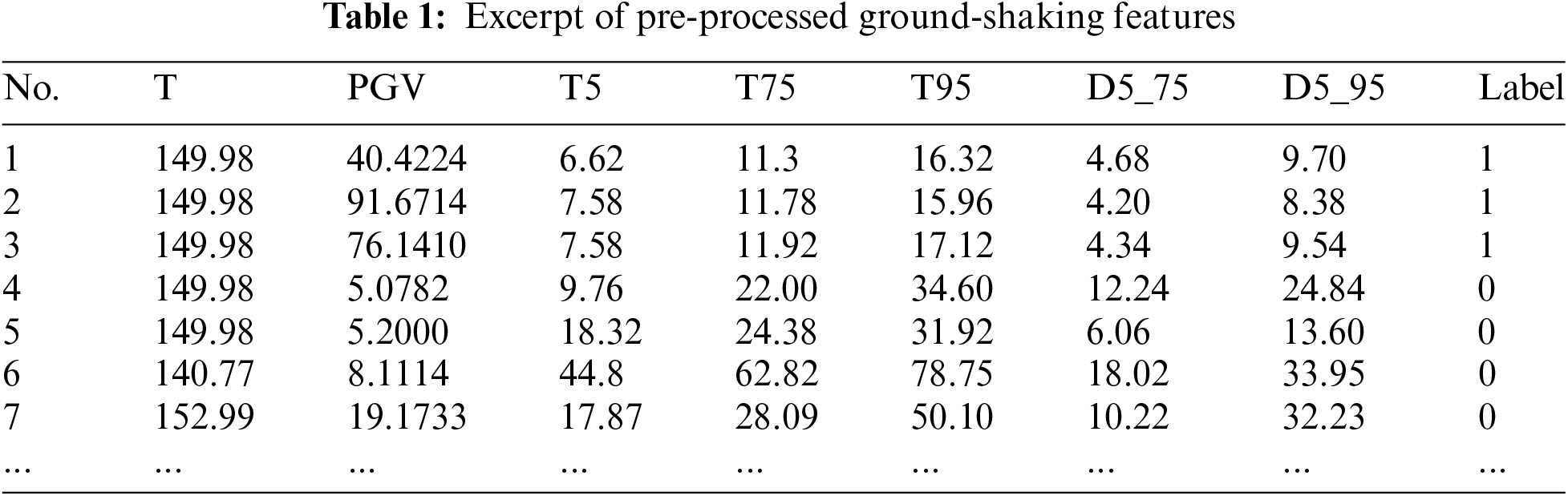
Comprehensively characterizing the ground-shaking data involves the consideration of several key eigenvalues, including the earthquake duration (T), PGV, time required for seismic intensity to reach the 5% (T5), 75% (T75), and 95% (T95) peaks, and the duration for the seismic intensity to transition from the 5% to 75% (D5_75) and 75% to 95% (D5_95) peaks. Due to the connection between the physical quantities, the velocity pulse data can reflect the characteristics of the acceleration pulse data to a certain extent. The introduction of the acceleration data can lead to a significant increase in computational complexity. Therefore, considering various factors, only the velocity pulse data was used as the input for this study. Additionally, for the purpose of facilitating both training and testing, the ground-shaking data was appropriately labeled (Section 2.1.2). A new ‘Label’ column was added to the dataset, with a value of 1 denoting impulsive ground-shaking and 0 denoting non-impulsive ground-shaking. After feature selection and labeling, the dataset for impulsive ground-shaking identification was completed (Table 1).

2.2 PCA

PCA is one of the most commonly used methods for complex input data processing and removing data with low correlations. The low-dimensional dataset output from PCA was mapped from the original high-dimensional dataset. The processed data reflected the key features of the original dataset to the greatest possible extent, reducing the risk of overfitting. Simultaneously, the PCA method downsizes the original data to reduce the volume and vastly improves the ANN training speed. In this study, due to the complexity of the ground-shaking data and the strong correlation between the different parameters, it is necessary to use PCA to reduce the number of parameters and maximize the retention of the key features of the original data to increase model training speed and identification efficiency.

The feature extraction steps for the ground-shaking data by PCA included: 1) data normalization; 2) covariance matrix calculation; 3) eigenvalue and eigenvector calculation; 4) eigenvalue ranking and selection; 5) dimensionality reduction and feature selection. Each of these steps is explained below in detail.

2.2.1 Data Standardization

Data standardization refers to the process of transforming data with different units and scales to scale-free data for comparability. For machine learning models, the scale difference will have a large impact on the model accuracy. Standardization makes the model more stable and accurate in training and prediction. In this study, the different entries of the ground-shaking data were corrected with large variations in parameter scales and distribution intervals by standardized transformations, to make values of the different parameters fall in an interval with small differences. The specific process is as follows.

Let S=[g1,g2,g3,…,gi,…,gn]T be the ground-shaking data description matrix, where gi represents the entries of all the system attributes in a certain operating state, i.e., an n-dimensional spatial vector describing a piece of ground-shaking data. By using xij to represent the elements of gi, the matrix M(xij) can be obtained as:

M=(x11x12…x1j…x1nx21x22…x2j…x2n⋮⋮⋱⋮⋮xi1xi2…xij…xin⋮⋮⋮⋱⋮xm1xm2…xmj…xmn).(5)

Subsequently, a standardization transformation is applied to all elements of the matrix:

xij¯=xij−μjσj,(6)

where xij¯ is the transformed data point; xij is the value of the ith parameter before the jth data correction; μj and σj are the mean and variance of all the parameters in column j of M(xij), respectively.

2.2.2 Covariance Matrix Calculation

Firstly, the covariance matrix is calculated for the normalized data, and the eigenvalues are obtained using the decomposition method. Then, the eigenvalues are sorted and the largest r eigenvalues are selected as the principal components (where r is the dimension after dimensionality reduction). Finally, the original data is linearly transformed using the selected principal components to map the high-dimensional data into the low-dimensional feature space. The specific processing flow is as follows:

If the ground-shaking data in the matrix is represented by xij, all elements, ρij, of the correlation coefficient matrix, R, can be computed as Eq. (7).

ρij=cov(xi¯,xj¯)σiiσjj,(7)

where

xi¯=1n∑i=1nxij,(8)

xj¯=1m∑i=1mxij.(9)

2.2.3 Eigenvalue and Eigenvector Calculation

A linear transformation can usually be fully described by the eigenvalues and eigenvectors. Therefore, in the PCA process, it is necessary to use the eigen-equations and eigenvectors to transform the vector space formed by the original data. In this method, the non-negative eigenvalues, λ1>λ2>⋯>λn, of R can be found from the eigen-equation, |R−λE|=0, where the eigenvectors of λi are [vi1,vi2,vi3,…,vin].

2.2.4 Eigenvalue Ranking and Selection

To indicate the reflection of the principal components on the original dataset information, the concepts of principal component and cumulative contribution ratios can be introduced in the selection process. They indicate the degree of expression of the original dataset information by using single and multiple principal components, respectively. The contribution ratio of the ith principal component can be defined as the proportion of its corresponding eigenvalue in the sum of all eigenvalues of the covariance matrix; the larger the contribution ratio, the stronger the ability of the ith principal component to synthesize the information of the original index. Let the eigenvalue of the ith principal component be λi. Then, the contribution ratio, Ai, of the ith principal component can be expressed as Eq. (10).

Ai=λi∑i=1nλi.(10)

By analogy, the weight of the sum of the eigenvalues of the first r principal components in the sum of all eigenvalues symbolizes their ability to summarize the information of the original data. Thus, in the method used in this study, the cumulative contribution, ηr, of the first r principal components can be expressed as Eq. (11).

ηr=∑i=1rλi∑i=1nλi.(11)

Comprehensively considering the accuracy and realistic conditions, when ηr reaches a value of 0.85, it is considered that the analytical accuracy meets the standard, and the use of the chosen r principal components meets the requirements for further analysis.

2.2.5 Downscaling and Feature Selection

Let the required principal component vector be Y1,Y2,Y3,…,Yr. If gi denotes the original n-dimensional vector describing the seismic data, the principal component vector can be expressed as Eq. (12).

Yi=v1gi+v2gi+v3gi+…+vngi(12)

2.3 LSTM

In this study, to identify impulsive ground-shaking, LSTM were used which are highly effective in processing time-series data.

2.3.1 Introduction to LSTM

LSTM is based on the development of recurrent neural networks (RNN). RNN is primarily used for sequence-type data. All the neurons in the hidden layer are connected in a chain structure, which is capable of realizing cyclic transmission of data in the network and memorizing the input data.

The horizontal structure of LSTM also forms a chain composed of repeated cellular units (Fig. 4), which maintains the memory function of RNN and effectively solves the gradient disappearance and long-range dependence problem of RNN through selective memorization and forgetting. Based on the classical RNN, the LSTM introduces memory cells for storing long-range dependency information along with forgetting, input, and output gates in a total of three gating unit layers in the hidden layer, which realize the addition and deletion of cell state information. Each gating unit contains a sigmoid activation function layer (σ in Fig. 4), with a value range of [0,1]: 0 means that the signal is not allowed to pass, and all the information is discarded, whereas 1 means that the signal is allowed to pass and the information is retained.

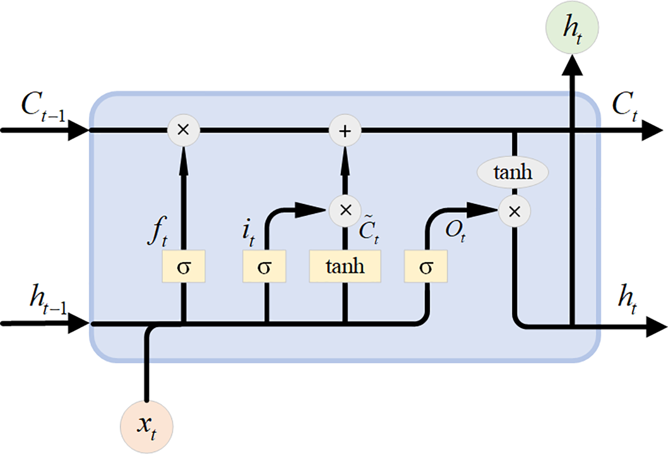
Figure 4: LSTM structure

2.3.2 LSTM Prediction Principles

The principle of the LSTM model for impulsive ground-shaking prediction mainly includes the following processes:

1)   Input ground-shaking data: The ground-shaking data at time t is input into the LSTM cell unit which is processed to obtain the signal output.

2)   Forgetting gate calculation: The hidden layer state, ht−1, of the previous moment and the input, a xt, of the current moment are read and the results are mapped to a range of [0,1] by the sigmoid activation function, whose value determines how much information is retained in the Ct−1 of the previous moment cell state. The forgetting gate discards the useless information in the Ct−1, and its output, ft is calculated as Eq. (13).

ft=σ(Wf⋅[ht−1,xt]+bf),(13)

where Wf is the corresponding weight matrix and bf is the bias term.

3)   Input gate calculation: The input gate determines the amount of information to be added to the cell state. It contains two layers: sigmoid and hyperbolic tangent (tanh). The hidden layer state, ht−1, of the previous moment and the input, xt, of the current moment are passed through the sigmoid layer to get the state value output, it, from the input gate, expressed as Eq. (14).

it=σ(Wi⋅[ht−1,xt]+bi).(14)

and the candidate cell state, C~t, is obtained through the tanh layer as Eq. (15).

C~t=tanh⁡(WC⋅[ht−1,xt]+bC),(15)

tanh⁡(x)=ex−e−xex+e−x,(16)

tanh′(x)=1−tanh2(x).(17)

4)   Update cell state: The cell state, Ct, at t is obtained by a linear operation of the forgetting gate, the output of the input gate, and the cell state at the previous moment. It can be expressed as Eq. (18).

Ct=ft⋅Ct−1+it⋅C~t.(18)

Output gate calculation: The hidden layer state, ht−1, of the previous moment and the input, xt, of the current moment are passed through the sigmoid layer, which produces the output, ot, at the output gate. The output gate controls the information of the cell state output. The cell state, Ct, at t is processed through the tanh layer, and the linear operation with ot is performed, expressed as Eq. (19).

ot=σ(Wo⋅[ht−1,xt]+bo),(19)

and the hidden layer state, ht, at t is finally obtained as Eq. (20).

ht=ot⋅tanh⁡(Ct),(20)

where Wo is the corresponding weight matrix and bo is the bias term.

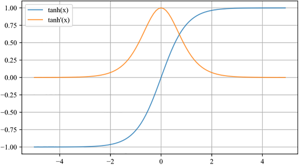
Figure 5: Plots of tanh (x) and tanh‵(x)

2.3.3 LSTM Model Training Principles

The predicted output of the LSTM model is then compared to the true results and the error between the two is calculated and back-propagated to update the model parameters. The error backpropagation is performed in the opposite direction to the forward propagation, i.e., layer by layer backpropagation from the output to the input layer. At each layer, the error backpropagation calculates the error gradient and accordingly updates the weights and thresholds. In this manner, the NN can gradually reduce the error and get progressively closer to the desired output. During the backpropagation process, by lending the output of the network to the previously delineated calibration result, the error of the network can be quantized using the cross-entropy loss function. The loss calculation process for a certain result can be expressed as Eq. (21).

Loss(Y^,Y)=−log⁡(eYi∑ieY^i)=−Yi+log⁡(∑ieY^i),(21)

where Loss is the error, Y^(i) is the network output, and Y(i) is the calibration result. Then, the gradients are computed for all the required variables and accumulated as Eq. (22).

grad(Y^)=∑i=1nddY^iLoss(Y^i,Yi),(22)

where n is the number of nodes in the output layer.

After deriving the quantized error, the NN (i) back-propagates layer by layer according to the error signal along the direction of the fastest descent of the relative error sum of squares, and (ii) calculates the adjustment amount and updates the weights and thresholds of each neuron, to allow the network outputs to gradually approximate the real value.

3  Experiment and Result Analysis

To validate the effectiveness of the proposed PCA-LSTM model, validation experiments based on the impulsive ground-shaking dataset constructed in Section 2 and analyzed the results. All the experiments performed in this study were conducted on a server with the following equipment configuration: (i) CPU: Intel(R) Core(TM) i5-12600K, (ii) GPU: NVIDIA GeForce RTX 3070, (iii) Windows 10 operating system, and (iv) algorithms and models written in Python.

3.1 PCA-LSTM Model Training

3.1.1 PCA

The PCA method can map high dimensional data to a lower dimension, and in the field of pulsed ground-shaking recognition, it can extract the most important features of impulsive ground-shaking, reduce the redundancy of data, highlight the key features, and help the LSTM model to better learn and understand the impulsive ground-shaking. The results after PCA of the ground-shaking data are shown in Table 2.

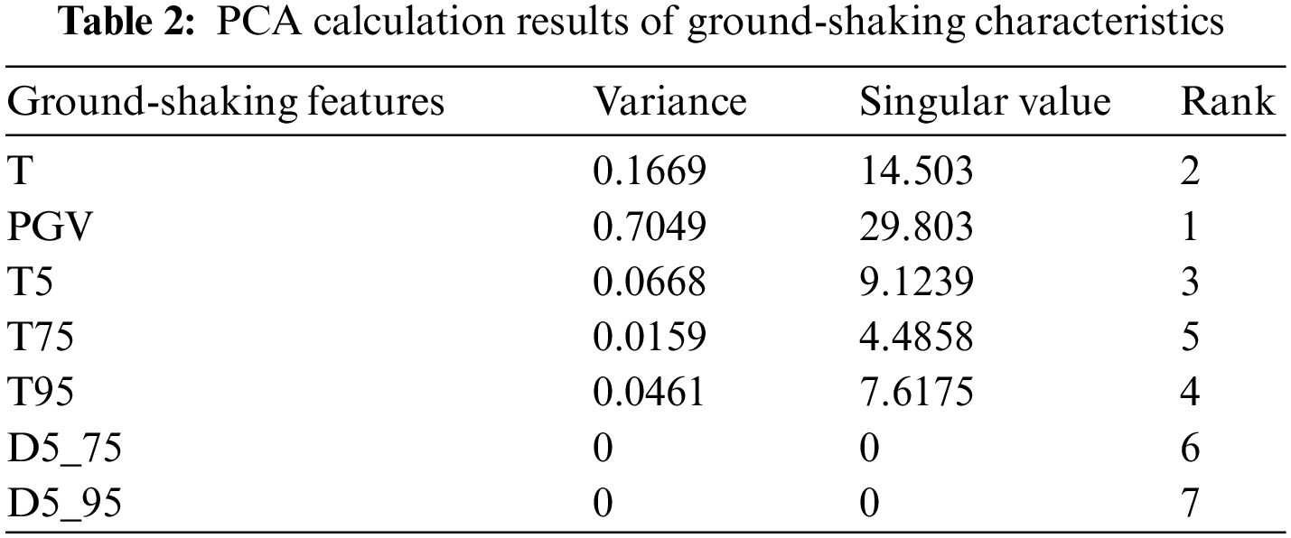
Finally, the ranking of the ground-shaking features was accomplished by PCA, and based on the calculated variance and singularity values, the top five ranked features, namely PGV, T, T5, T95, and T75, were selected as the five eigenvalues, which were used as the inputs for the subsequent LSTM model training.

3.1.2 LSTM Model Training

In order to guarantee optimal model performance, attention should be given to enhancing the model’s generalizability and mitigating overfitting during the training process. The dataset based on PCA to extract the main features was randomly divided into the training, validation, and test sets in a ratio of 7:1:2. Among these, the training set was used to train the LSTM model and update the model parameters for the model to determine whether it contains impulsive ground-shaking data points based on the input data; the validation set was used to evaluate the model accuracy and generalization performance during the training process; and the test set was used to evaluate the accuracy and generalizability of the completed training model. Normally, the validation and test sets are not involved in model updation.

When training the LSTM model, the parameters need to be defined, including the number of model training rounds, the choice of optimizer, batch size, and so on (Table 3). The variation of the training and validation loss during the training of the LSTM model is shown in Fig. 6.

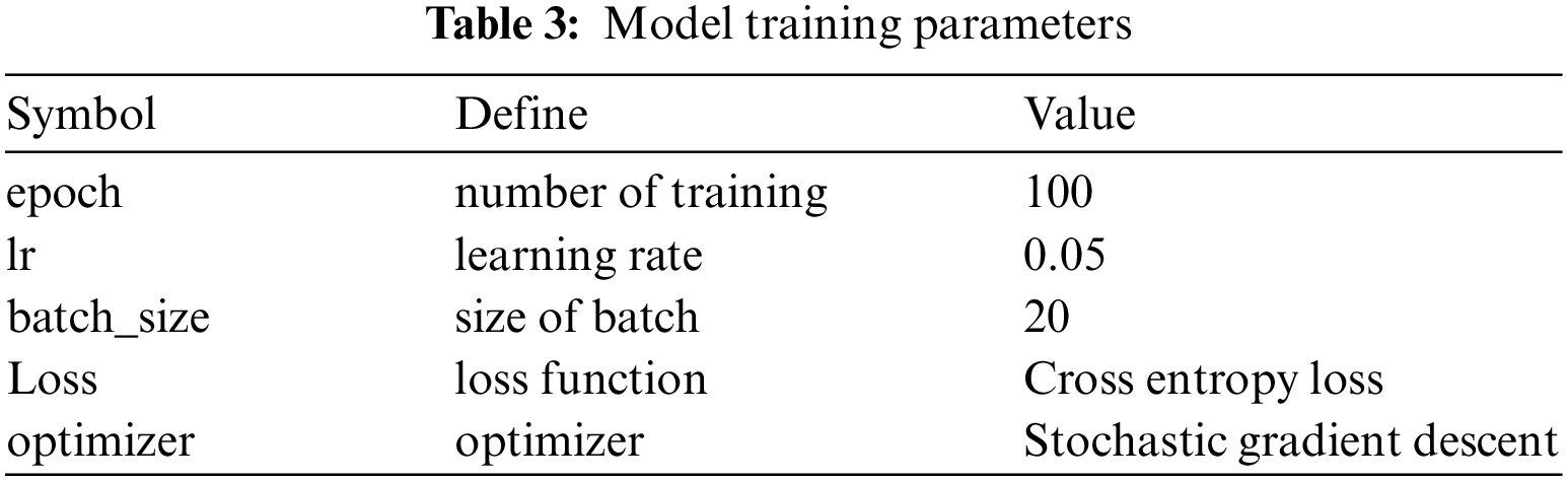
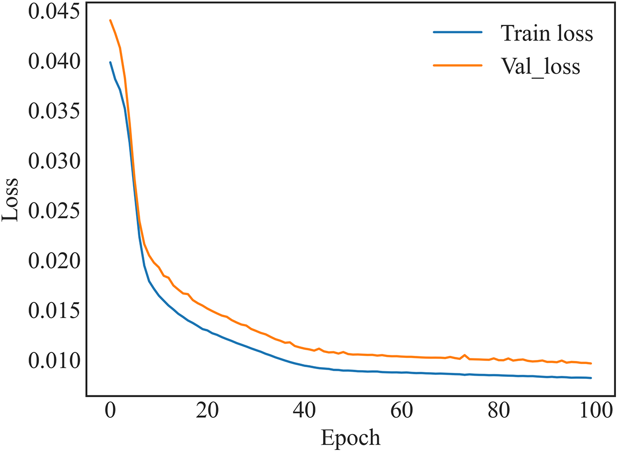
Figure 6: Variation of loss during LSTM model training

Both loss metrics of the LSTM model gradually decreased and stabilized during the training process. After ~50 iterations, both training and validation losses plateaued. Eventually, the training loss stabilized at 0.010 and the validation loss stabilized at ~0.012. It can be seen that the model not only obtains good performance on the training set, but also has a good fitting effect on the validation set, verifying the generalizability of the model.

3.2 Comparative Analysis of Models

3.2.1 Indicators of Model Assessment

To further verify the PCA-LSTM model performance, the evaluation system for the impulsive ground-shaking identification was constructed, and the model was comprehensively evaluated in terms of two important factors, i.e., accuracy rate Eq. (23) and identification speed Eq. (24). A high accuracy rate implies that the algorithm can accurately determine which ground-shaking signals are impulsive. Low accuracy will lead to misclassification and under-classification problems, which may result in misinterpretation of earthquakes and lead to risks in earthquake engineering designs. Earthquakes are unexpected events, and accurate and timely identification of impulsive ground shaking is crucial for taking emergency measures and activating the earthquake early warning system. A high-speed impulsive ground-shaking identification model can analyze seismic signals in real-time and respond quickly to provide accurate seismic parameters, thus helping to mitigate the damage caused by earthquakes.

P=TT+F×100%(23)

where P, T, and F denote the accuracy rate of identification, the number of accurate and inaccurate identifications of ground-shaking data.

S=data_sizetime(24)

where S donates the identification speed of the model, data_size denotes the size of the dataset, i.e., the number of ground-shaking data points in the test set, and time denotes the time required for the model to predict the dataset.

3.2.2 Comparison of Models

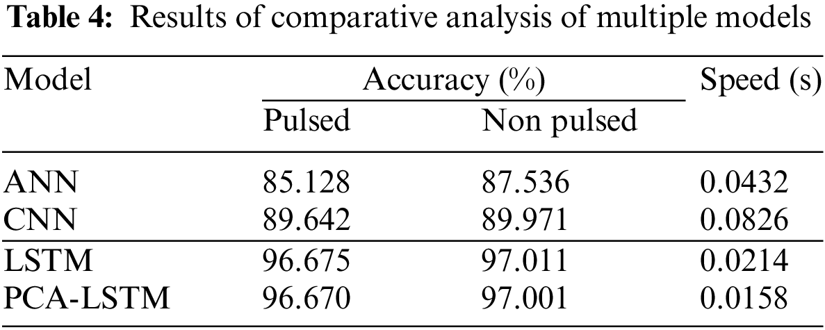
To further illustrate the advantages of the proposed PCA-LSTM model, it was trained using the same training set and parameters as the ANN, CNN, and LSTM models. Comparative analyses were then performed for the same test set and the evaluation metrics described in Section 3.2.1 were used for the assessment. The results of the comparative analyses involving the multiple models are presented in Table 4. The recognition accuracy of the LSTM model for impulsive and non-impulsive ground-shaking improved by >7.033% and >7.040%, respectively, compared to the other two models. The LSTM model was more accurate than the ANN and CNN models as it has a good analytical processing capacity for time series data. The reason why the identification accuracy for the non-impulsive ground-shaking was higher than that of impulsive ground-shaking was mainly due to the abundance of the former data in the training set, which trains the model more comprehensively. When comparing LSTM and PCA-LSTM models, it becomes evident that the latter maintains model identification accuracy while enabling low-dimensional data input. Additionally, the identification speed of the model improved by 26.168% compared to LSTM due to the reduced dimensionality of the input data. These findings demonstrated that the proposed model offers significant advantages in terms of both accuracy and speed, affirming its effectiveness. The research conducted in this study provides a new solution in the field of ground-shaking identification.

4  Discussion

Currently, due to limitations in resources, energy, and external conditions, certain shortcomings in the presented work remain. The following aspects will need to be further investigated:

•   Ground-shaking signals exhibit various features across different frequency ranges. Future research can explore effective methods for integrating these multi-scale features to harness both global and local characteristics of the ground-shaking signals.

•   Subsequent research efforts may consider incorporating data augmentation techniques, model integration methods, and anomaly detection algorithms to enhance the robustness and reliability of the model.

5  Conclusion

To accurately and efficiently recognize impulsive ground-shaking and reduce the damage to engineering structures, a combined DL recognition model, named PCA-LSTM, was introduced in this paper. The detailed information of the model is presented as follows:

1.    The model construction was mainly based on the analysis and identification of impulsive ground-shaking features and the annotation of the ground-shaking data using the traditional method proposed by Baker [9].

2.    Training and testing of the model: After constructing the ground-shaking dataset, the most relevant ground-shaking features were extracted using the PCA method. Subsequently, the ground-shaking dataset was updated and only the extracted feature values were retained. This reduced data redundancy and improved the efficiency of model training and identification. Finally, the reconstructed dataset was divided, trained, and analyzed for comparison.

3.    Advantages: Compared to other benchmark models, the proposed PCA-LSTM model showed excellent performance in terms of identification accuracy and speed. It greatly improved the accuracy and speed of pulsed ground-shaking identification. In addition, the model can be applied to solve practical engineering problems. It is of great significance for seismic monitoring and structural engineering design, thus, improving our ability to mitigate seismic hazards to a certain extent and safeguarding lives and property.

Acknowledgement: None.

Funding Statement: The author received no specific funding for this study.

Author Contributions: The author confirms contribution to the paper as follows: study conception and design: Yizhao Wang; data collection: Yizhao Wang; analysis and interpretation of results: Yizhao Wang; draft manuscript preparation: Yizhao Wang. All authors reviewed the results and approved the final version of the manuscript.

Availability of Data and Materials: The ground-shaking data used in this paper was obtained from the earthquake database provided by the United States Geological Survey (USGS).

Conflicts of Interest: The author declare that he has no conflicts of interest to report regarding the present study.

References

1. Anderson, J. C., Bertero, V. V. (1987). Uncertainties in establishing design earthquakes. Journal of Structural Engineering, 113(8), 1709–1724. [Google Scholar]

2. Hall, J. F., Heaton, T. H., Halling, M. W., Wald, D. J. (1995). Near-source ground motion and its effects on flexible buildings. Earthquake Spectra, 11(4), 569–605. [Google Scholar]

3. Kuo, C. H., Huang, J. Y., Lin, C. M., Hsu, T. Y., Chao, S. H. et al. (2019). Strong ground motion and pulse-like velocity observations in the near-fault region of the 2018 Mw 6.4 Hualien, Taiwan, earthquake. Seismological Research Letters, 90(1), 40–50. [Google Scholar]

4. Wang, J. Z., Zhu, X. (2003). Acceleration-sensitive region under pulsational ground motion near seismic source. China Railway Science, 24(6), 27–30. [Google Scholar]

5. Somerville, P., Saikia, C., Wald, D., Graves, R. (1996). Implications of the Northridge earthquake for strong ground motions from thrust faults. Bulletin of the Seismological Society of America, 86(1B), S115–S125. [Google Scholar]

6. Furumura, T., Koketsu, K. (1998). Specific distribution of ground motion during the 1995 Kobe earth- quake and its generation mechanism. Geophysical Research Letters, 25(6), 785–788. [Google Scholar]

7. Wang, Y. J., Ma, K. F. (2015). Investigation of the temporal change in attenuation within the ruptured fault zone of the 1999 mw7. 3 Chi-Chi, Taiwan earthquake. Pure and Applied Geophysics, 172, 1291– 1304. [Google Scholar]

8. Zhang, X., Zha, X., Dai, Z. (2015). Stress changes induced by the 2008 Mw 7.9 Wenchuan earthquake. Journal of Asian Earth Sciences, 98, 98–104. [Google Scholar]

9. Baker, J. W. (2007). Quantitative classification of near-fault ground motions using wavelet analysis. Bulletin of the Seismological Society of America, 97(5), 1486–1501. [Google Scholar]

10. Chang, Z., Sun, X., Zhai, C., Zhao, J. X., Xie, L. (2016). An improved energy-based approach for selecting pulse-like ground motions. Earthquake Engineering & Structural Dynamics, 45(14), 2405–2411. [Google Scholar]

11. Zhao, G., Xu, L., Xie, L. (2016). A simple and quantitative algorithm for identifying pulse-like ground motions based on zero velocity point method. Bulletin of the Seismological Society of America, 106(3), 1011–1023. [Google Scholar]

12. Huang, Y., Fu, J. (2019). Review on application of artificial intelligence in civil engineering. Computer Modeling in Engineering & Sciences, 121(3), 845–875. https://doi.org/10.32604/cmes.2019.07653 [Google Scholar] [CrossRef]

13. Deng, X., Shao, H., Hu, C., Jiang, D., Jiang, Y. (2020). Wind power forecasting methods based on deep learning: A survey. Computer Modeling in Engineering & Sciences, 122(1), 273–301. https://doi.org/10.32604/cmes.2020.08768 [Google Scholar] [CrossRef]

14. Sircar, A., Yadav, K., Rayavarapu, K., Bist, N., Oza, H. (2021). Application of machine learning and artificial intelligence in oil and gas industry. Petroleum Research, 6(4), 379–391. [Google Scholar]

15. Reichstein, M., Camps-Valls, G., Stevens, B., Jung, M., Denzler, J. et al. (2019). Deep learning and process understanding for data-driven earth system science. Nature, 566(7743), 195–204. [Google Scholar] [PubMed]

16. Wang, J., Sun, P., Chen, L., Yang, J., Liu, Z. et al. (2023). Recent advances of deep learning in geological hazard forecasting. Computer Modeling in Engineering & Sciences, 137(2), 1381–1418. https://doi.org/10.32604/cmes.2023.023693 [Google Scholar] [CrossRef]

17. Jozinović, D., Lomax, A., Štajduhar, I., Michelini, A. (2020). Rapid prediction of earthquake ground-shaking intensity using raw waveform data and a convolutional neural network. Geophysical Journal International, 222(2), 1379–1389. [Google Scholar]

18. Zhang, G., Lin, C., Chen, Y. (2020). Convolutional neural networks for microseismic waveform classification and arrival picking. Geophysics, 85(4), WA227–WA240. [Google Scholar]

19. Chen, Y., Zhang, G., Bai, M., Zu, S., Guan, Z. et al. (2019). Automatic waveform classification and arrival picking based on convolutional neural network. Earth and Space Science, 6(7), 1244–1261. [Google Scholar]

20. Ku, B., Min, J., Ahn, J. K., Lee, J., Ko, H. (2020). Earthquake event classification using multitasking deep learning. IEEE Geoscience and Remote Sensing Letters, 18(7), 1149–1153. [Google Scholar]

21. Hochreiter, S., Schmidhuber, J. (1997). Long short-term memory. Neural Computation, 9(8), 1735–1780. [Google Scholar] [PubMed]

22. Hao, Z. (2017). Network data feature selection research and simulation optimization method. Computer Simulation, 34, 367–370. [Google Scholar]

23. Shin, T. C., Teng, T. L. (2001). An overview of the 1999 Chi-Chi, Taiwan, earthquake. Bulletin of the Seismological Society of America, 91(5), 895–913. [Google Scholar]

24. Yu, Y. X., Gao, M. T. (2001). Effects of the hanging wall and footwall on peak acceleration during the Jiji (Chi-ChiTaiwan Province, earthquake. Acta Seismologica Sinica, 14(6), 654–659. [Google Scholar]

25. Wang, W. L., Wang, T. T., Su, J. J., Lin, C. H., Seng, C. R. et al. (2001). Assessment of damage in mountain tunnels due to the Taiwan Chi-Chi earthquake. Tunnelling and Underground Space Technology, 16(3), 133–150. [Google Scholar]

26. Hung, J. J. (2000). Chi-Chi earthquake induced landslides in Taiwan. Earthquake Engineering and Engineering Seismology, 2(2), 25–33. [Google Scholar]

27. Lin, J. L. (2022). Power responses of a building subjected to pulse-like ground motions. Earthquake Engineering & Structural Dynamics, 51(2), 457–472. [Google Scholar]

28. Tang, Y., Wu, C., Wu, G. (2021). Automated detection of velocity pulses in ground motions based on adaptive similarity search in response spectrum. Soil Dynamics and Earthquake Engineering, 149, 106626. [Google Scholar]

29. Chang, Z., Gao, Q., Monti, G., Yu, H., Yuan, S. (2023). Selection of pulse-like ground motions with strong velocity-pulses using moving-average filtering. Soil Dynamics and Earthquake Engineering, 164, 107574. [Google Scholar]

30. Ghanbari, B., Fathi, M. (2022). Extraction of velocity pulses of pulse-like ground motions using empirical fourier decomposition. Journal of Seismology, 26(5), 967–986. [Google Scholar]