Maximum Correntropy Criterion-Based UKF for Loosely Coupling INS and UWB in Indoor Localization

1  Introduction

Indoor localization technology has important applications in modern society. As the need for indoor positioning accuracy and reliability increases dramatically, researchers are committed to developing more efficient and accurate indoor positioning methods. The Inertial Navigation System (INS) and Ultra-Wideband (UWB) techniques are two common methods for indoor localization, each with its own set of advantages and limitations.

The Inertial Navigation System (INS) is a self-sufficient navigation technology that operates independently without reliance on external information or the emission of external energy. This autonomy endows it with unique advantages, such as being inconspicuous and immune to external electromagnetic interference. Inertial Navigation utilizes an inertial measurement unit (IMU), a technology that estimates position, velocity, and attitude by fusing acceleration and angular velocity. The Inertial Navigation System (INS) relies on sensors like accelerometers and gyroscopes to gauge an object’s acceleration and angular velocity. This data allows for the continuous and real-time tracking of position and attitude. Nonetheless, as time progresses, cumulative errors begin to accumulate, becoming increasingly significant with extended durations. Ultra-Wideband technology can realize centimeter-level high-precision distance measurement. However, in indoor environments, the path of signal propagation is non-line-of-sight stemming from various obstacles such as furniture, decorations, pillars, doors, and partitions. At this point, UWB is unable to achieve accurate distance measurement and position estimation. The fusion localization scheme based on UWB/INS, on the one hand, compensates for the loss of accuracy of UWB localization in the non-line-of-sight (NLOS) environment and smoothes the localization trajectory of UWB; on the other hand, it also eliminates the aggregated error of INS and augments the localization precision of INS. The integrated system can also output multi-dimensional data such as position, velocity and attitude, which enriches the positioning information. In this research paper, the application of the Kalman filter is explored. Nonetheless, these filters, which are developed using the minimum mean square error (MMSE) approach, may not adequately accommodate the unpredictable noise encountered in UWB scenarios, leading to potentially significant errors. To triumph over this dilemma, this paper presents a novel approach utilizing the unscented Kalman filter (UKF) algorithm incorporating the maximum correntropy criterion (MCC).

Linear dynamic systems usually use the Kalman filter (KF), but when dealing with nonlinear problems, the extended Kalman filter (EKF) [1] and the unscented Kalman filter (UKF) [2] are commonly used. EKF algorithm linearizes nonlinear functions using Taylor series expansion, replacing the state transfer matrix with the Jacobi matrix in Kalman filtering equations. Then, it calculates state estimation and variance within the Kalman filtering framework. However, this approximation may not be sufficiently accurate, especially when the function shows a high degree of nonlinearity, which can potentially lead to filter divergence. In addition, the derivation of the Jacobi matrix is very cumbersome and can be difficult to implement. The Unscented Kalman filter (UKF) algorithm uses the Unscented Transform to derive a set of sigma points. It then converts the task of linearizing the nonlinear function into approximating the probability density distribution of the system’s state variables through nonlinear function transfer. Finally, it addresses the filtering issue within the framework of the Kalman filter algorithm. The UKF method offers a derivative-free, higher-order approximation that can achieve more precise results without requiring the computation of the complex Jacobi matrix unlike EKF. However, both EKF and UKF may not be effective in scenarios where the measurement is affected by heavy-tailed non-Gaussian noise. To address this issue, robust methods like Huber’s generalized great likelihood method have been proposed in [3,4], which combines both l1/l2 paradigms to construct the cost function and can minimize the maximum asymptotic estimation variance for the case of disturbed Gaussian distributions, and its robustness is better than that of the estimation based on the l2 paradigm while trying to keep the l2 paradigm for a pure Gaussian distribution as much as possible estimation efficiency when pure Gaussian distribution is maintained as much as possible. In contrast, the maximum correntropy-based nonlinear unscented Kalman filter (MCCUKF) derived in this paper utilizes UT to obtain the prediction state estimates, and the measurement information is reformulated using the nonlinear regression model under MCC, considering the covariance matrix. Subsequently, the filter states and covariance matrix are obtained through UT applied to the measurement equations. The paper presents an advanced fusion localization method for INS and UWB, combining EKF and MCCUKF for enhanced robustness in complex environments, unlike previous studies using single or linear filters. A new clustering algorithm is also introduced to reduce UWB’s non-line-of-sight ranging errors.

The paper presents the following contributions:

1)   We proposed a new clustering algorithm: k-medoid clustering based on bisection k means to preprocess UWB data and remove outliers caused by ranging errors or noise interference, making the positioning results more accurate.

2)   Applying the unscented Kalman filter based on the maximum correntropy criterion to indoor positioning to complete the fusion of ultra-wideband and inertial Navigation.

3)   A dual filtering algorithm based on maximum correntropy unscented Kalman filter and extended Kalman filter is proposed to loosely couple the localization results of INS and UWB while achieving more accurate and stable indoor localization.

The subsequent sections of the paper are structured as follows. In the next section, we present the work on the localization algorithm. Section 3 describes the proposed localization and clustering algorithms and derives the numerical expressions for the MCCUKF localization algorithm. Section 4 compares and analyzes the simulation results of various algorithms and the experiment result. Finally, Section 5 gives conclusions and an outlook for future research.

2  Related Work

Table 1 summarizes related works with different fusion types of indoor localization.

Target tracking and localization are necessary in the fields of satellite network orbiting and autonomous Navigation, network communication, mobile position estimation, and wireless sensor network motion target tracking [12]. The loose coupling method is relatively straightforward and uncomplicated. On the contrary, although tight coupling has higher positioning accuracy, it requires more algorithms and computational resources, and the time synchronization requirement between INS and UWB is relatively high, which needs to ensure that the data acquisition and processing time of both are consistent. Tight coupling has higher positioning accuracy compared to loose coupling, but there are still difficulties in practical realization. In [13], the authors proposed a Fixed Lag Extended Finite Impulse Response Smoothing (FEFIRS) algorithm to integrate the INS and UWB data tightly. Most classical filtering theories, such as least squares filtering, assume that Gaussianity is its underlying distribution [3]. The authors of [14] first proposed a multi-hypothesis starting location discrimination method based on observability analysis, which assists in attaining precise starting points. By suppressing the severe linearization loss in conventional EKFs, antics-EKF helps to improve ballistic tracking accuracy. LS-SVM-assisted UFIR filters were proposed in [15]. The authors in [16] transformed the RWSL problem into a nonconvex optimization problem without the need for statistical NLOS errors and path states. A hybrid skeleton-based wireless localization and placement technology of reference nodes, known as integrated wireless location, was put forward by [17].

Compared with RSSI, channel status information (CSI) can effectively avoid the adverse effect of the multipath effect on the localization results. Therefore, the value of CSI is used as the feature value of localization, the location fingerprint database of Radio Map is established, and the weighted proximity algorithm matches the recent fingerprint database data of KNN to estimate the location of the localization point. Reference [18] proposed a Gramer-Rao lower bound (CRLB) approach based on CSI localization. Reference [19] identified the fundamental differences in the physical layer between Bluetooth Low Energy (BLE) BLE and Wi-FI, and proposes the Bloc system, which combines novel, BLE-compatible algorithms to customer service the challenges of extending CSI localization to BLE. In [20], the authors put forward a new deep learning-based approach for indoor vehicle localization (Deep VIP) using the smartphone’s built-in sensors for indoor vehicle localization. The authors in [21] introduced a novel method for indoor localization by integrating dictionary learning techniques. This framework was further enhanced with a Hidden Markov-based tracking algorithm, elevating the precision of the solution.

In recent research, numerous scholars have incorporated the concept of correntropy into the field of indoor localization. The maximum correntropy principle argues that in the absence of a priori knowledge, we should choose the probability distribution with maximum uncertainty. In indoor localization, the maximum correntropy criterion can be employed to estimate the uncertainty of the location and incorporate it into the design of the filter. Reference [22] introduced a method for automatically selecting regularization parameters in the maximum correntropy criterion (MCC) by incorporating a general convex regularization penalty term in the situation where pre-existing knowledge, such as state constraints, is available. In [23], the authors proposed a novel approach by combining the maximum correntropy criterion Kalman filter (MCC-KF) with the estimation projection method. In [24], an extended kernel recursive maximum correntropy adaptive filtering algorithm was put forward to strengthen resistance to interference of the system to non-Gaussian noise. The authors in [25] proposed an improved K-medoids clustering algorithm which preserves the computational efficiency and simplicity of the simple and fast K-medoids algorithm while improving its clustering performance. In [26], the authors proposed a loosely coupled fusion of INS and UWB based on generalized probabilistic data association (GPDA) with a modified verification gate (MVG) based on conventional GPDA.

3  Proposed Algorithm

The intention of this paper is to accommodate a loosely coupled integrated high-accuracy localization system for INS and UWB in the indoor environment. Generally, the inertial navigation system mounts the inertial element on the mobile node (MN). As the node moves, its angular velocity changes constantly. The inertial element’s gyroscope is capable of measuring the MN’s angular momentum. By applying knowledge of dynamics, this data can be used to determine the heading angle and attitude of the MN during movement. Additionally, the accelerometer can measure the acceleration of MN through primary and secondary integration over time. One can obtain the velocity and position information of the MN during its motion. For each UWB subsystem, the distance connecting MN and BS is measured using the time-of-arrival (TOA) technique. This distance data is then preprocessed using the k-medoid clustering method based on bisection k, which means discarding the outliers with large errors and attenuating the ramification of NLOS on the positioning validity. Afterward, the UWB position estimation is obtained by utilizing the trilateral measurement method. Finally, the dual filtering algorithms, namely the extended Kalman filter (EKF) and the maximum correntropy-based unscented Kalman filter (MCCUKF), are employed to fuse INS and UWB data. The overall framework is portrayed in Fig. 1.

Figure 1: The flowchart of recommended algorithm

3.1 INS Navigation

INS is an environmentally independent navigation technique. In INS, the coordinate system for attitude detection is commonly used as a carrier coordinate system and navigation coordinate system. In the theory of rigid body fixed point rotation, the attitude modes describing the kinematic coordinate system are Euler angles, quaternions, and directional cosines. The inertial measurement unit (IMU) collects acceleration and angular velocity data in three axes through the accelerometer and gyroscope built into the INS, respectively. It should be emphasized that the acceleration data is the information in connection with the carrier’s coordinate system. Therefore, to accurately determine the position and velocity of the Mobile Node (MN), it is essential to transform the acceleration data into information applicable to the navigational coordinate system. Angular velocity information is typically used to update the attitude of the Mobile Node (MN) and thus does not require conversion between coordinate systems. Euler angles are used to provide information about the MN’s orientation. ε=[φθϕ]T, φ is roll, θ is pitch, and ϕ is yaw. ν=[νnνeνd]T is the velocity vector and the position vector is P =[pnpepd]T. n, e, d denote the east, north, and down directions, respectively. From the knowledge of the dynamics of the robotic arm, the state transfer equation of the robotic arm was obtained, and from the accelerometer and gyroscope measurements, the attitude, velocity and position information of the robotic arm was estimated, the state vectors are as stated below:

xτ=[εTvTpTbwTbaT]T(1)

where, bwT signifies the gyroscope bias and baT signifies the accelerometer bias. The motion model of INS is presented below:

xτ=[εTvTpTbωTbAT]T=[12qT⊗(ωT−bωT)Cbn(AT−bAT)+gTvT00](2)

where, q is the quaternion form of the attitude information of the mobile node, ⊗ is the quaternion product, Cbn is the directional cosine matrix, ω and A are the gyroscope and accelerometer measurements, respectively, and g is the gravitational acceleration, the error state model of the MN is

Δxτ=[ΔεTΔvTΔpTΔbωTΔbAT]T=[−[ωT−bωT]×ΔεT−ωω−Cbn[AT−bAT]×ΔεT−CbnΔbωTΔvTωωaω](3)

where, Δxτ is the error state vector, Δε represents the error in attitude, Δv represents the error in velocity, Δp represents the error in position, respectively. Δbω, ΔbA are the errors of the gyroscope and accelerometer, [⋅]× is the skew symmetry operator, ωω represents the stochastic disturbance of the gyroscope , Aω represents the stochastic disturbance of the accelerometer. The error state vector corrects the state vector through feedback, as shown in the flowchart in Fig. 1.

3.2 UWB Navigation

3.2.1 Signal Model

The available UWB ranging models are Received Signal Strength (RSS), Time of Arrival/Time Difference of Arrival/Round Trip Time of Flight (TOA/TDOA/RTOF), and Phase Difference of Arrival (PDOA). In this paper, the Time of Arrival (TOA) is used for UWB distance measurement. Assuming that the number of base stations involved in localization is M and the coordinates are j = 1, 2,…, M, the base station receives signals from the mobile node, the TOA is modeled as follows:

dj(τ)={djtrue(τ)+Nτlosconditiondjtrue(τ)+dnlos+Nτnloscondition(4)

djtrue(τ)=||PjBS−PτMN||(5)

where, dj(τ) is the geographical separation between the j-th base station and the mobile node at the τ instance. djtrue(τ) is the precise distance between j-th base station and the mobile node at τ instance. Nτ represents the LOS measurement error which modeled as the Gaussian white noise whose mean value is zero and the standard deviation is σg2, dnlos represents the error caused by NLOS transmission which modeled as a gamma distribution, as shown in (6).

f(dNLOS)=α2exp⁡(−α2dNLOS)(α2dNLOS)α1−1Γ(α1)(6)

where α1 is the shape parameter, α2 is the scale parameter, PτMN=[x^τMNy^τMNz^τMN] is the mobile node’s coordinate. So, the dNLOS’s means value and dNLOS’s standard deviation is α1α2,α1α22, respectively.

3.2.2 K-Medoid Based on Bisection K-Means

The distance measurements of UWB contain NLOS errors and measurement errors, which can cause serious errors in the localization results if this result is directly used for subsequent localization. It is imperative to mitigate the impact of NLOS on the localization results following the distance measurement. This paper introduces a novel algorithm for NLOS suppression to preprocess the obtained distance values, replacing some of the measurement values containing NLOS errors with those not interfered with by NLOS. In the k-means algorithm, we repeatedly select the cluster’s mean as the new center and continue iterating until the cluster’s objects’ distribution remains unchanged. In contrast, the k-medoid algorithm selects the points in the sample as the clustering center each time. This paper’s objective is to enhance the precision and stability of clustering outcomes by presenting a k-medoid clustering approach that utilizes bisection k-means. The method first performs bisection k-mean clustering on the ranging values, takes the clustering result of the bisection k-mean as a known point, then calculates the distance from this known point to each point in the sample, and selects the sample point closest to the known point as the initial clustering center. By adopting this approach, we can enhance the accuracy of selecting the initial cluster center and thus improve the quality of the clustering results.

To implement bisection k-medoid clustering on the data, we set the number of clusters k to 4. Select the two clusters with the smallest sum of squared errors (SSE) and compute the centers of the clusters. It is important to note that in k-medoid clustering, the center of mass for each cluster must be an actual data point, and these initial centers are chosen randomly. However, this random selection can lead to instability and the problem of local optima in the k-medoid algorithm. To address this, our paper introduces an algorithm for selecting the k-medoid cluster centers, with the process outlined as follows:

Step 1: At the τ moment, record the L distance measurement values including both LOS measurement values and NLOS measurement values between the j-th base station and the mobile node as

Dj=[dj,1BS_MN(τ)dj,2BS_MN(τ)⋯dj,LBS_MN(τ)](7)

Step 2: The L measurements are grouped into a single cluster, which is then divided into two sub-clusters, after which the cluster Vi with the largest sum of squared errors (SSE) is selected, and the cluster is binary clustering with the underlying k-means. This process of division is continued until the number of clusters reaches 4. The formula for the sum of squared errors (SSE) is given below:

SSE=∑i=1κ⁡∑y∈Vi⁡dist(νi,y)2(8)

where, νi is the clustering center of cluster Vi, and y is the sample in the cluster.

Step 3: From the final four clusters, the two clusters V1 and V2 with the smallest SSE are selected, and the centers μ1 and μ2 of the clusters are computed to obtain the clustering results with bisection k-means: μ=[μ1μ2].

Step 4: Calculate the distance from μ=[μ1μ2] to each sample data point and select the closest sample point to μ as the original cluster centroid of k-medoid for k-medoid clustering. Note that the cluster grouping for k-medoid clustering is 2. The L distance values are classified into two categories, LOS and NLOS. By k-medoid, to obtain the clustering center λ1 for LOS and the clustering center λ2 for NLOS. Measurements greater than λ2 are replaced with λ2, thereby attenuating the effect of NLOS.

The flowchart of our clustering algorithm is portrayed in Fig. 2.

Figure 2: The flowchart of k-medoid based on bisection k-means

3.2.3 UWB Location

Trilateral measurements and least squares are introduced to deduce the coordinates of MN. The location coordinates of the base station and MN are PjBS and PτMN, respectively. Note that zjBS=zτ, from Eq. (9), we get

{(x1BS−x^τMN)2+(y1BS−y^τMN)2=D^1(τ)(x2BS−x^τMN)2+(y2BS−y^τMN)2=D^2(τ)⋮(xMBS−x^τMN)2+(yMBS−y^τMN)2=D^M(τ)(9)

We represent the above equation using a linear matrix

ΛPMN=Π(10)

where, Λ,P MN and Π are

Λ=2[(x1BS−x2BS),(y1BS−y2BS)(x1BS−x3BS),(y1BS−y3BS)⋮(x1BS−xMBS),(y1BS−yMBS)](11)

PMN=[x^τMNy^τMN](12)

Π=[D^2(τ)2−D^1(τ)2−(x2BS2+y2BS2)+(x1BS2+y1BS2)D^3(τ)2−D^1(τ)2−(x3BS2+y3BS2)+(x1BS2+y1BS2)⋮D^M(τ)2−D^1(τ)2−(xMBS2+yMBS2)+(x1BS2+y1BS2)](13)

Finally, the position of MN at moment n is estimated as

[x^τMN,y^τMN]T=(ΛTΛ)−1ΛTΠ(14)

3.3 Maximum Correntropy Criterion

3.3.1 Introduction of MCC

Correntropy, a novel concept, is employed to evaluate the overall similarity between two random variables. Considering two specified random variables Υ11var,Υ2var∈R, whose joint density function is FΥ1var,Υ2var(y1var,y2var), and whose correntropy is defined as

V(ϒ1var,ϒ1var)=E[κσ(Υ1var,Υ2var)]=∫∫κσ(y1var,y2var)dFΥ1var,Υ1var,(y1var,y2var)(15)

where, E[⋅] is the expectation operator and κ(⋅) denotes a shift-invariant kernel following the Mercer condition. The main role of the kernel function is to compute the inner product of two input variables after dimensional transformation. Therefore, any kernel function can be rewritten as κσ(y1var,y2var)=⟨Φ(y1var),Φ(y2var)⟩. Here, ⟨⋅⟩ denotes the inner product is computed. Φ(x) is a mapping function used to map the data to different dimensions. Each kernel function corresponds to a unique mapping function. In this research paper, we opt for the widely used Gaussian kernel as the kernel function. The mathematical expression for the Gaussian kernel is as follows:

κσ(y1var,y2var)=Gσ(ℓ)=exp(−ℓ22σ2)(16)

where, ℓ=y1var−y2var, and σ>0 is the kernel bandwidth which is a very important design parameter in MCC.

Correntropy can be gauged by utilizing the sample mean estimator at N specified points.

V^(Υ1var,Υ2var)=1N∑i=1NGσ(ℓ(i))(17)

where, ℓ(i)=y1var(i)−y2var(i), with {y1var(i),y2var(i)}i=1N denotes the sample drawn from the joint density function FΥ1var,Υ2var,(y1var,y2var). When we perform Taylor series expansion on the Gaussian kernel function.

V(Υ1var,Υ2var)=∑n=0∞⁡(−1)n2nσ2nn!E[(Υ1var−Υ2var)2n](18)

The concept of correntropy becomes apparent. Correntropy is defined as the summation of weighted even-order moments of the error variable. Additionally, the kernel bandwidth plays a significant role as a parameter that determines the importance of statistical instances of order two and higher. It is important to note that when the kernel bandwidth greatly surpasses the data’s dynamic range. Considering a time series of residuals {ℓ(i)}i=1N, the cost function of the MCC can be portrayed as mentioned below:

JMCC=1N∑i=1N⁡Gσ(ℓ(i))(19)

3.3.2 Comparison to Minimum Mean Square Error (MSE) Criterion

A comparison of the formulas for the minimum mean square error criterion and the maximum correntropy criterion is as follows:

MSE(Υ1var,Υ2var)=E[(Υ1var−Υ2var)2]=∫∫(y1var−y2var)2dFΥ1var,Υ2var(y1var,y2var)(20)

V(Υ1var,Υ2var)=E[κσ(Υ1var,Υ2var)]=∫∫κσ(y1var,y2var)dFΥ1var,Υ2var(y1var,y2var)(21)

It is evident that the minimum mean square error criterion is a quadratic function in random space in the joint probability density along the y1var=y2var perimeter, i.e., the integral of the error. However, there are certain problems with utilizing a quadratic measure of difference. If some of the samples between the random variables are farther away from y1var=y2var, then one will amplify this error in a quadratic fashion, making the effect of these samples far greater than the effect of the other samples, making the gap between the two samples wider and wider. The Gaussian correntropy limits the infinite expansion of this error since the Gaussian function has a value range of (0,1], so the effect on individual samples is limited to this interval. The kernel function is the form of its limitation. To a certain extent, the correntropy of the differences in the individual samples will be reflected more evenly.

3.4 MCCUKF-Based INS/UWB Integration

3.4.1 EKF Prediction

Navigation information from INS and UWB is fused by quadratic filtering based on EKF and MCCUKF. Specifically, the state transfer equation and observation equation of MCCUKF are first constructed based on the output of EKF. Then, the nonlinear function is mapped onto a Gaussian distribution using the traceless transform, and the state estimation and update are performed through the prediction and update steps. Finally, more accurate position estimation results are obtained by MCCUKF fusion. The error state prediction and prediction covariance are given below:

Δx^τ|τ−1ekf=ψτ|τ−1(Δx^τ|τ−1ekf,uτ−1)+ξ,ξ∼N(0,Q⌣)(22)

Pτ|τ−1ekf=ψτ|τ−1Pτ−1|τ−1ekfψτ|τ−1T+Q⌣τ|τ−1(23)

Q⌣=diag[Ng2Nf2Ngδb2Nfδb2](24)

where, ψτ|τ−1=I+Fτ|τ−1δt is the discrete-time state transfer matrix, and uτ−1=(ωτ−1T,Aτ−1T)T is the input vector of the system. ξ is the Gaussian white noise of the system with a covariance matrix of Q⌣. Ng and Nf is the random noise in gyroscopes and accelerometers, Ngδb and Nfδb is dynamic bias in gyroscopes and accelerometers, respectively. Q⌣τ|τ−1=G⌣Q⌣τ−1|τ−1G⌣Tδt, F is the continuous time state transfer matrix shown in (25). δt is the sampling interval of IMU and G⌣ is control matrix as formulated in (26).

F=[Cbτ|τ−1n[ωτ−1T−bωT]×00Cbn0Cbτ|τ−1n[Aτ−1T−bAT]×000−Cbn0I3000000−1ℜω00000−1ℜA](25)

G=[Cbτ|τ−1n0000−Cbτ|τ−1n00000000I30000I3](26)

where, Cbτ|τ−1n is the updated DCM calculated from the latest updated attitude. ℜω and ℜA are correlation times of the gyroscope and accelerometer. The given observation model is expressed as follows:

zτ=H⌣Δx^τ|τ−1ekf+r,r∼N(0,R⌣)(27)

γτ=zτ−H⌣Δx^τ|τ−1ekf(28)

Sτ=H⌣Δx^τ|τ−1ekfH⌣T+R⌣(29)

where, zτ is the observation vector at the moment τ, H⌣ is the observation matrix given by (30), r is the observation error with the covariance matrix of R⌣, Sτ is the covariance matrix of innovation.

H⌣=[00I300](30)

3.4.2 EKF Update

The Kalman gain is giving by

Kτekf=Pτ|τ−1ekfH⌣T(Sτ)−1(31)

The error state is updated as below:

Δx^τ|τekf=Kτekfγτ=Kτekf(zτ−H⌣Δx^τ|τ−1ekf)(32)

Covariance update:

Pτ|τekf=(I−KτekfH⌣)Pτ|τ−1ekf(33)

3.4.3 MCCUKF Prediction

The error equations of state and observation equations for discrete-time nonlinear systems are

Δx^τ=f(τ,Δx^τ−1)+ντ−1(34)

zτ=h(τ,Δxτ)+mτ(35)

where, Δx^τ∈Rn1 stands for the n1-dimensional system’s error state vector at τ moment. zτ∈Rn2 stands for the measurement vector with n2 dimensions. f(x) and h(x) are system function and measurement function. Process noise ντ−1 and measurement noise mτ are uncorrelated with each other. Both the stochastic disturbance and measurement noise have zero mean and are characterized by their respective covariance matrices.

ντ:E[ντ]=0,E[vτ−1vτ−1T]=Qτ−1mτ:E[mτ=0],E[mτmτT]=Rτ(36)

When performing MCCUKF prediction, the initial state is the output state of the first stage of INS/UWB fusion using EKF, i.e., Δx^0|0=Δx^τ|τekf , and the starting covariance matrix is P0|0=P0|0ekf, 2L+1 sigma points are then obtained by performing an unscented transformation on Δx^τ−1|τ−1 and Pτ−1|τ−1, which can be represented by

χτ−1|τ−1s={Δx^τ−1|τ−1s=0Δx^τ−1|τ−1+((L+λ)Pτ−1|τ−1)ss=1,2,…,LΔx^τ−1|τ−1−((L+λ)Pτ−1|τ−1)ss=L+1,…,2L(37)

where, L denotes the dimension of the state vector, λ=α2(L+φ)−L is scale correction factor, where, α determines the degree of diffusion of the sigma point, in general, 0<α≤1, φ is a scaling factor usually set to 3−L. The constant λ determines the distribution of sigma points around Δx^τ−1|τ−1.

Using the 2L+1 sigma above to obtain the priori error state and the priori state covariance matrix, the following equations are obtained

Δx^τ|τ−1=∑s=02L⁡wmsf(τ−1,χτ−1|τ−1s)(38)

Pτ|τ−1=∑s−02L⁡wcs[f(τ−1,χτ−1|τ−1s)−Δx^τ|τ−1]×[f(τ−1,χτ−1|τ−1s)−Δx^τ|τ−1]T+Qτ(39)

wm0=λ(L+λ),wc0=λ(L+λ),wms=wcs=12(L+λ),s=1,…,2L.(40)

where, β is associated with the prior knowledge of the Δx^τ distribution (β=2 is considered to be the most optimal).

3.4.4 MCCUKF Measurement Update

A collection of sigma points is derived from the priori error state prediction mean Δx^τ|τ−1 and covariance matrix Pτ|τ−1

χτ|τ−1s={Δx^τ|τ−1s=0Δx^τ|τ−1+((L+λ)Pτ|τ−1)ss=1,2,…,LΔx^τ|τ−1−((L+λ)Pτ|τ−1)ss=L+1,…,2L(41)

Afterwards, the forecasted measurement mean is determined as shown below:

z^τ=∑s=02L⁡ωmsh(τ,χsτ|τ−1),s=0,…,2L(42)

Furthermore, the state measurement cross-covariance matrix is as follows:

Pxz=∑s=02L⁡ωcs[χsτ|τ−1−Δx^τ|τ−1][h(τ,χsτ|τ−1)−z^τ]T(43)

Subsequently, we utilize MCC to execute the observation update. Initially, we denote the priori estimation error of the state as

ζ(Δxτ)=Δx^τ|τ−1−Δxτ(44)

Combining Eqs. (34), (35) and (44), we obtained the following statistical nonlinear regression model.

[Δx^τ|τ−1zτ]=[Δxτh(τ,Δxτ)]+ξ~τ(45)

where, ξ~τ is

ξ~τ=[ζ(Δxτ)mτ](46)

with

Θτ=E[ξ~τξ~Tτ] =[Pτ|τ−100R(τn)] =[Bτ|τ−1P(Bτ|τ−1P)T00Bτr(Bτr)T] =BτBτT(47)

where, Bτ can be obtained by the Cholesky decomposition of Θτ, Left-multiplying Bτ−1 on both sides of the Eq. (45), we get the transformed statistical regression model.

Dτ=g(τ,Δxτ)+eτ(48)

where,

Dτ=Bτ−1[Δx^τ|τ−1zτ],g(τ,Δxτ)=Bτ−1[Δxτh(τ,Δxτ)],eτ=Bτ−1ξ~τ.(49)

We proceed by formulating a cost function utilizing MCC.

JM(Δxτ)=∑s=1M⁡Gσ(dτs−gs(τ,Δxτ))(50)

where, dτs is the s-th element of Dτ, gs(τ,Δxτ) is the s-th row of g(τ,Δxτ), and M=n1+n2 is the dimension of Dτ. Based on the nature of the correlation entropy, the optimal approximation of the state can be obtained when the function JM(⋅) is taken to be the maximum

Δx^τ=arg⁡maxΔxτJM(Δxτ)=arg⁡maxΔxτ∑s=1M⁡Gσ(eτe)(51)

where, eτe is the s-th element of eτ given as follows:

eτs=dτs−gs(τ,Δxτ)(52)

The optimal solution of Δxτ is obtained by taking the partial derivative of JM(Δxτ) with respect to Δxτ and making it zero:

∂JM(Δxτ)∂Δxτ=0(53)

This can alternatively be stated below:

∑s=1M⁡φ(eτs)∂eτs∂Δxτs=0(54)

When Δxτs is the i-th element of Δxτ, and φ(eτs)=Gσ(eτs)⋅eτs. Then, we define C(τ,s)=φ(eτs)/eτs and then come up with the following formula:

C(τ,s)=Gσ(eτs)(55)

The Eq. (54) can be further written in the form of a matrix as

(∂g(τ,Δxτ)∂Δxτ)TCτ[Dτ−g(τ,Δx(τn)τ)]=0(56)

where, Cτ=[CτP00Cτr], Cτ(i)P and Cτ(i)r are calculated as shown below:

Cτ(i)P=[G(eτ1)⋯0⋮⋱⋮0⋯G(eτn1)]Cτ(i)r=[G(eτn1+1)⋯0⋮⋱⋮0⋯G(eτn1+n2)](57)

where, i represents the number of iterations.

Define Θ~τ as the revised covariance, which can be depicted as

Θ~τ=BτCτ−1BτT(58)

Next, write Θ~τ in two portions so that

Θ~τ=[Θ~τP00Θ~τr](59)

The actual state Δxτ is not known. we set ζ(Δxτ)=Δxτ−Δx^τ|τ−1=0. In this way, it is easy to derive

Θ~τP=Bτ|τ−1P∗I∗(Bτ|τ−1P)T=Pτ|τ−1(60)

The revised measurement covariance is

R¯τ=Θ~τr(61)

The state equation and measurement equation can be further written as

Status update:

Δx^τ|τ=Δx^τ|τ−1+Kτ(zτ−z^τ)(62)

Covariance update:

Pτ|τ=P¯τ|τ−1−KτPzzKτT(63)

where,

{K τ=PxzPzz−1P¯τ|τ−1=Bτ|τ−1P(CτP)−1(Bτ|τ−1P)−1(64)

The autocorrelation matrix

Pzz=∑s=02L⁡wcs[h(τ,χsτ|τ−1)−z^τ][h(τ,χsτ|τ−1)−z^τ]T+R¯τ(65)

As a result, the nominal state of the MT is calibrated as follows and the final state estimate is produced:

x^τ|τ=x^τ−Δx^τ|τ(66)

4  Simulation and Experiment

In this chapter, the effectiveness of the suggested solution is evaluated by simulation results.

4.1 Simulation

In the conducted experiment, five beacon nodes are randomly arranged in the scene, using NaveGo as a simulation tool. The target node follows a predetermined trajectory in the simulation scene. The range of the simulation scene is 60m×60m. Since only the localization accuracy of the two-dimensional plane is considered in the experiments in this paper, the z-coordinate is set as a constant of 2m in the simulation. This simulation modeling experiment ignores the positioning error in the vertical direction and considers only the planar coordinates. The simulation study was conducted to investigate the non-line-of-sight errors obeying the gamma, Gaussian and uniform distributions, respectively. EKF [27], Joint-state estimate Particle Filter (JSEPF-EKF) [28], PF [29] and Classical-UKF [30] are used as comparative algorithms to validate the effectiveness of the suggested solution, and Cumulative Error Distribution Function (CDF) and Root Mean Square Error (RMSE) are used as the criteria for evaluating the effectiveness of different algorithms.

RMSE=1T⋅tm∑i=1tm⁡∑τ=1T⁡||xτ(7:9)−x^τ|τ(7:9)||2(67)

where, T=16282 is the total number of samples, tm is the number of Monte Carlo runs. xτ(7:9) is the actual coordinates of the mobile node at the τ-th simulation, x^τ|τ(7:9) is the predicted coordinates of the mobile node obtained by the proposed algorithm of this paper at the τ-th simulation. The simulation outcomes were obtained through over 1000 iterations of the Monte Carlo method. The filter parameter settings and specifications for IMU and UWB is depicted in Table 2.

4.1.1 Gamma Distribution

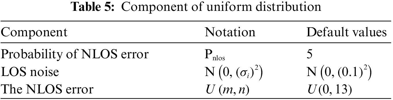
We make the assumption that the measurement noise’s distribution is Gaussian, and when the non-line-of-sight error obeys a gamma distribution, the components for the simulation are set as presented in Table 3.

The following simulation results are analyzed:

By referring to Fig. 3, it can be seen that when the probability of NLOS error increases from 0.1 to 0.8, the RMSE of EKF, JSEPF-EKF and PR-PF increases expeditiously with the gradual increase of NLOS probability, and the average accuracy of localization are 1.818, 1.762 and 2.207 m, respectively. Whereas the proposed solution’s average localization precision is 0.821 m, the average localization precision of Classical-UKF is 0.8093 m. The average localization precision of the proposed solution is improved by 54.84%, 53.41% and 62.80% compared to EKF, JSEPF-EKF and PR-PF, respectively. When the probability of non-line-of-sight error is between 0.3 and 0.7, the localization accuracy of Classical-UKF is higher than that of MCCUKF.

Figure 3: The value of the corresponding RMSE changes with the variation of NLOS error’s probability

Fig. 4 shows that the RMSE of EKF, JSEPF-EKF, Classical-UKF and PR-PF increases significantly when NLOS error’s mean value increases gradually from 1 to 6, while the proposed solution increases slowly and shows a relatively smooth effectiveness. The mean localization inaccuracies of the EKF, JSEPF-EKF, Classical-UKF and PR-PF are 1.771, 1.812, 1.157 and 2.1 m, respectively, whereas that of the proposed solution is 0.5746 m. In comparison to the other three comparative algorithms, the proposed solution demonstrates noteworthy progress in accuracy, with enhancements of 67.56%, 68.28%, 50.33% and 72.64% compared to EKF, JSEPF-EKF, Classical-UKF and PR-PF, respectively. It is evident that the proposed solution manifests superior localization accuracy and robustness when compared to the other three algorithms.

Figure 4: The value of the corresponding RMSE changes with the variation of NLOS error’s mean value

As depicted in Fig. 5, with the increasing standard deviation of NLOS, the RMSE of EKF, JSEPF-EKF, PR-PF and Classical-UKF shows a slow increasing trend, with average inaccuracies of 1.996, 1.929, 2.31 and 0.8157 m, respectively. The RMSE of the proposed solution shows a slow decreasing trend with little change and the average error is 0.541 m. The positioning performance of MCCUKF is superior to that of the Classic-UKF.

Figure 5: The value of the corresponding RMSE changes with the variation of NLOS error’s standard deviation

Fig. 6 shows that the average inaccuracies of all algorithms have several distinct peaks. This is because the rotation occurs during the movement of the MN when there is an abrupt change in the motion state of the MN. The average inaccuracies of EKF, JSEPF-EKF, PR-PF and Classical-UKF are 1.937, 1.829, 2.311 and 1.206 m, respectively. In contrast, the proposed solution’s average inaccuracy is 0.593 m, The positioning error is 1.344, 1.236, 1.718 and 0.613 m lower than the four comparative algorithms, and the precision is improved by 69.39%, 67.58%, 74.34% and 49.60%, respectively.

Figure 6: The average RMSE over time

Fig. 7 depicts the cumulative probability of the proposed algorithm reaches 1 very quickly, and the localization inaccuracies are distributed within 0.5 m from the target point.

Figure 7: The relationship between the CDF and the location error

4.1.2 Gaussian Distribution

When the measurement noise and the NLOS error both follow a Gaussian distribution, the corresponding parameters are set, as portrayed in Table 4.

Fig. 8 shows that the larger the NLOS error probability is, the larger the localization inaccuracy is and the smaller the accuracy is. The mean localization inaccuracies of EKF, JSEPF-EKF, PR-PF and Classical-UKF are 3.294, 2.957, 3.214 and 1.232 m, respectively. The accuracies of the proposed solution are improved by 81.41%, 79.29%, 80.94% and 50.28%, respectively, as compared to EKF, JSEPF-EKF, PR-PF and Classical-UKF.

Figure 8: The value of the corresponding RMSE changes with the variation of NLOS error’s probability

Fig. 9 shows that the RMSE of the proposed solution stays around 0.5 m, which has smaller and more stable localization inaccuracy. The EKF, JSEPF-EKF, PR-PF and Classical-UKF algorithms exhibit average localization errors of 3.678, 3.597, 3.627 and 0.6798 m, respectively. In contrast, the proposed solution achieves an average localization accuracy with an inaccuracy rate of 0.487 m. Comparing it with the other four algorithms, the proposed solution showcases accuracy improvements of 86.76%, 86.43%, 86.57% and 28.36%, respectively.

Figure 9: The value of the corresponding RMSE changes with the variation of NLOS error’s standard deviation

In Fig. 10, when NLOS error’s the mean value is between 3 and 9, the RMSE of the proposed solution is around 0.5 m, and the accuracy is improved by 87.12%, 87.10%, 87.37% and 28.11% compared to EKF, JSEPF-EKF, PRPF and Classical-UKF, respectively. Obviously, the solution presented in this paper demonstrates superior localization precision and robustness.

Figure 10: The value of the corresponding RMSE changes with the variation of NLOS error’s mean value

The CDF of the location error was depicted in Fig. 11. The proposed solution achieves a localization inaccuracy of approximately 0.9 m, surpassing the other four algorithms in terms of its significantly enhanced localization accuracy.

Figure 11: The relationship between the CDF and the location error

4.1.3 Uniform Distribution

Assuming that the LOS error follows a Gaussian distribution N(0,σG2) and the NLOS error follows a uniform distribution U(m,n), the conventional parameter settings are as portrayed in Table 5.

In Fig. 12, the localization accuracy of all algorithms shows a decreasing trend with increasing NLOS error probability. Compared to EKF, Classical-UKF, JSEPF-EKF and PRPF, the proposed solution exhibits improvements in accuracy by 79.24%, 20.08%, 79.16% and 81.39%, respectively. Besides, compared to the Classical-UKF, the MCCUKF has a slightly better positioning performance.

Figure 12: The value of the corresponding RMSE changes with the variation of NLOS error’s probability

At higher NLOS probability, the localization error is also increasing. However, the solution suggested can lower the impact of NLOS error on the localization effectiveness, so that the effectiveness remains better under higher NLOS probability, which indicates that the proposed solution demonstrates greater robustness and adaptability.

In Fig. 13, the RMSE of the EKF,JSEPF-EKF, PR-PF exhibits an increase as the NLOS standard deviation increases. However, the RMSE of the algorithm presented in this paper remains relatively stable around 0.5 m, with no notable changes. The proposed solution in this paper demonstrates improved accuracy compared to EKF, JSEPF-EKF, and PR-PF, with enhancements of 84.89%, 84.59%, and 86.01%, respectively, while it improves 32.09% over the Classical-UKF. From the simulation results in Fig. 13, it can be seen that the performance of UKF is improved by adding the maximum correntropy criterion.

Figure 13: The value of the corresponding RMSE changes with the variation of NLOS error’s standard deviation

In Fig. 14, the CDF plot of the proposed solution shows a steep shape, which indicates that most of the samples have a small localization error. This implies that the proposed algorithm exhibits enhanced effectiveness in localization.

Figure 14: The relationship between the CDF and the localization error

4.2 Experiment

To verify the efficacy of the suggested solution in localization, we established an authentic experimental setting within the library and the classroom. The distance separating the mobile node from the base station is measured by the TOA-based ranging technique through UWB wireless communication technology utilizing narrowband pulse transmission data characteristics. Considering the requirements of low cost and high effectiveness. The INS sensor comprises a triaxial gyroscope and a triaxial accelerometer, which can gauge the acceleration and angular velocity of the corresponding axes. Figs. 15 and 16 show the UWB module and inertial navigation trolley. To handle the time synchronization issue between the UWB module and the INS, the mobile node is prevented from traveling on the inertial navigation trolley and synchronized with the trolley. As shown in Figs. 17, 18, 19a and 19b, the experimental scenarios are the library and the classroom. We arranged five base stations, and the trolley containing the mobile nodes traveled along a predetermined trajectory, whose speed is 0.5 m/s at a uniform speed. The trajectory of the cart is represented by the red line and the arrow is the direction of movement The frequency of UWB in the experiment is 5 Hz, and the number of samples in the library and classroomis 294 and 322, respectively. The INS has a sampling frequency of 50 Hz and the number of samples in library and classroom is 2946 and 3220, respectively. The initial coordinates of the x-axis, y-axis and z-axis are set as 0.6, 0.6, and 0.2 m, correspondingly.

Figure 15: The UWB node

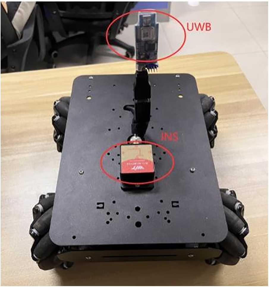
Figure 16: Inertial navigation trolley

Figure 17: Experimental scenario (library)

Figure 18: Experimental scenario (classroom)

Figure 19: The experiment’s floor plan

As depicted in Fig. 20, the suggested solution exhibits a significantly lower average localization error compared to the four algorithms being compared. Specifically, Fig. 20a shows that in the library, the average errors for EKF, JSEPF-EKF, Classical-UKF and PR-PF are recorded as 2.422, 2.199, 1.358 and 1.632, respectively, the proposed algorithm achieves an average error of 1.158. Fig. 20b shows that in the classroom, the average errors for EKF, JSEPF-EKF, Classical-UKF and PR-PF are recorded as 4.275, 4.683, 1.63 and 3.563, respectively, whereas the proposed algorithm achieves an average error of only 1.006. The CDF in Fig. 21 also clearly depicts that the suggested solution significantly outperforms the other comparative algorithms in terms of localization accuracy.

Figure 20: Positioning deviations of different sampling point

Figure 21: The relationship between the CDF and the localization error, (a) is in the library, (b) is in the classroom

5  Conclusion

In this research, a novel approach for enhancing the precision and reliability of indoor localization is introduced. The proposed method combines maximum correntropy with unscented Kalman filtering for inertial Navigation and an integrated ultra-wideband localization system. We first proposed a k-medoid clustering algorithm based on bisection k-means to preprocess UWB data and remove outliers caused by ranging errors or noise interference. Then, the concept of maximum correntropy criterion is implemented in the unscented Kalman filter, and the solutions of the inertial navigation system and the ultra-wideband system are fused using a hybrid filter based on EKF and MCCUKF to derive the ultimate state estimation of the target. The algorithm described in this paper exhibits enhanced precision and robustness in localization. Although the proposed algorithm has good performance in single-target localization, in multi-target localization, the performance of the algorithm is degraded due to the interactions between targets. Future research will concentrate on assessing the algorithm’s effectiveness in complex environments, such as multi-target tracking.

Acknowledgement: The authors wish to express their appreciation to the editors and reviewers for their helpful review and recommendations which greatly improved the presentation of this paper.

Funding Statement: This work was supported by the National Natural Science Foundation of China under Grant Nos. 62273083 and 61803077; Natural Science Foundation of Hebei Province under Grant No. F2020501012.

Author Contributions: The authors confirm contribution to the paper as follows: Guidance and oversight throughout the project: Yan Wang; provide critical feedback on the manuscript: Yan Wang; study conception and design: You Lu; data collection: You Lu; analysis and interpretation of results: You Lu; experimental design and perform data analysis: You Lu, Yuqing Zhou, Zhijian Zhao; draft manuscript preparation: You Lu. All authors reviewed the results and approved the final version of the manuscript.

Availability of Data and Materials: All the reviewed research literature and used data in this research paper consists of publicly available scholarly articles, conference proceedings and reports. The references and citations are contained in the reference list of this manuscript. Any further inquiries about the data can be directed to the corresponding author.

Conflicts of Interest: The authors declare that they have no conflicts of interest to report regarding the present study.

References

1. Feng, D., Wang, C., He, C., Zhuang, Y., Xia, X. G. (2020). Kalman-filter-based integration of IMU and UWB for high-accuracy indoor positioning and navigation. IEEE Internet of Things Journal, 7(4), 3133–3146. https://doi.org/10.1109/jiot.2020.2965115 [Google Scholar] [CrossRef]

2. Yin, H. H., Xia, W. W., Zhang, Y. Y., Shen, L. F. (2016). UWB-Based indoor high precision localization system with robust unscented kalman filter. 2016 IEEE International Conference on Communication Systems (ICCS), Shenzhen, China, IEEE. [Google Scholar]

3. Petrus, P. (1999). Robust huber adaptive filter. IEEE Transactions on Signal Processing, 47(4), 1129–1133. https://doi.org/10.1109/78.752610 [Google Scholar] [CrossRef]

4. Wang, H. W., Li, H. B., Zhang, W., Zuo, J. Y., Wang, H. P. (2019). Derivative-free Huber-Kalman smoothing based on alternating minimization. Signal Processing, 163, 115–122. https://doi.org/10.1016/j.sigpro.2019.05.011 [Google Scholar] [CrossRef]

5. Cho, S. Y., Lee, J. H., Park, C. G. (2022). Maximum correntropy criterion-based UKF for tightly coupling INS and UWB with non-Gaussian uncertainty noise. ICINCO, pp. 209–213. Lisbon, Portugal. [Google Scholar]

6. Bu, L., Zhang, Y., Xu, Y., Chen, X. (2018). Robust tightly-coupled INS/UWB-integrated human localization using UFIR filtering. 2018 IEEE International Instrumentation and Measurement Technology Conference (I2MTC), pp. 1–5. Houston, TX, IEEE. [Google Scholar]

7. Zeng, Z., Liu, S., Wang, L. (2018). NLOS detection and mitigation for UWB/IMU fusion system based on EKF and CIR. 2018 IEEE 18th International Conference on Communication Technology (ICCT), pp. 376–381. Chongqing, China, IEEE. [Google Scholar]

8. Zhao, H., Tian, B., Chen, B. (2022). Robust stable iterated unscented Kalman filter based on maximum correntropy criterion. Automatica, 142, 110410. https://doi.org/10.1016/j.automatica.2022.110410 [Google Scholar] [CrossRef]

9. Hafez, I., Wadi, A., Abdel-Hafez, M. F., Hussein, A. A. (2023). Variational Bayesian-based maximum correntropy cubature Kalman filter method for state-of-charge estimation of Li-ion battery cells. IEEE Transactions on Vehicular Technology, 72(3), 3090–3104. https://doi.org/10.1109/tvt.2022.3216337 [Google Scholar] [CrossRef]

10. Liu, X., Song, C. T., Pang, Z. H. (2022). Kernel recursive maximum correntropy with variable center. Signal Processing, 191, 108364. https://doi.org/10.1016/j.sigpro.2021.108364 [Google Scholar] [CrossRef]

11. Wang, X. Y., Gao, L. J., Mao, S. W., Pandey, S. (2017). CSI-based fingerprinting for indoor localization: A deep learning approach. IEEE Transactions on Vehicular Technology, 66(1), 763–776. https://doi.org/10.1109/tvt.2016.2545523 [Google Scholar] [CrossRef]

12. Liu, X., Ren, Z., Lyu, H., Jiang, Z., Ren, P. et al. (2021). Linear and nonlinear regression-based maximum correntropy extended Kalman filtering. IEEE Transactions on Systems Man Cybernetics-Systems, 51(5), 3093–3102. https://doi.org/10.1109/tsmc.2019.2917712 [Google Scholar] [CrossRef]

13. Xu, Y., Shmaliy, Y. S., Ahn, C. K., Shen, T., Zhuang, Y. (2021). Tightly coupled integration of INS and UWB using fixed-lag extended UFIR smoothing for quadrotor localization. IEEE Internet of Things Journal, 8(3), 1716–1727. https://doi.org/10.1109/jiot.2020.3015351 [Google Scholar] [CrossRef]

14. Zhao, W., Zhao, H., Liu, G., Zhang, G. (2022). ANFIS-EKF-based single-beacon localization algorithm for AUV. Remote Sensing, 14(20), 5281. https://doi.org/10.3390/rs14205281 [Google Scholar] [CrossRef]

15. Xu, Y., Li, Y., Ahn, C. K., Chen, X. (2020). Seamless indoor pedestrian tracking by fusing INS and UWB measurements via LS-SVM assisted UFIR filter. Neurocomputing, 388, 301–308. https://doi.org/10.1016/j.neucom.2019.12.121 [Google Scholar] [CrossRef]

16. Chen, H. T., Wang, G., Ansari, N. (2019). Improved robust TOA-based localization via NLOS balancing parameter estimation. IEEE Transactions on Vehicular Technology, 68(6), 6177–6181. https://doi.org/10.1109/tvt.2019.2911187 [Google Scholar] [CrossRef]

17. Chiu, C. J., Chan, F. C., Feng, K. T. (2022). Skeleton-based positioning and reference point deployment for hybrid wireless localization. IEEE Transactions on Vehicular Technology, 71(5), 5404–5414. https://doi.org/10.1109/tvt.2022.3153166 [Google Scholar] [CrossRef]

18. Gui, L. Q., Yang, M. X., Yu, H., Li, J., Shu, F. et al. (2018). A Cramer-rao lower bound of CSI-based indoor localization. IEEE Transactions on Vehicular Technology, 67(3), 2814–2818. https://doi.org/10.1109/tvt.2017.2773635 [Google Scholar] [CrossRef]

19. Ayyalasomayajula, R., Vasisht, D., Bharadia, D. (2018). BLoc: CSI-based accurate localization for BLE tags. Proceedings of the 14th International Conference on Emerging Networking Experiments and Technologies, pp. 126–138. Heraklion, Greece. [Google Scholar]

20. Zhou, B. D., Gu, Z. N., Gu, F. Q., Wu, P., Yang, C. J. et al. (2022). DeepVIP: Deep learning-based vehicle indoor positioning using smartphones. IEEE Transactions on Vehicular Technology, 71(12), 13299–13309. https://doi.org/10.1109/tvt.2022.3199507 [Google Scholar] [CrossRef]

21. Kumar, C., Rajawat, K. (2019). Dictionary-based statistical fingerprinting for indoor localization. IEEE Transactions on Vehicular Technology, 68(9), 8827–8841. https://doi.org/10.1109/tvt.2019.2929360 [Google Scholar] [CrossRef]

22. Zhang, X., Li, K. X., Wu, Z. Z., Fu, Y. L., Zhao, H. Q. et al. (2016). Convex regularized recursive maximum correntropy algorithm. Signal Processing, 129, 12–16. https://doi.org/10.1016/j.sigpro.2016.05.030 [Google Scholar] [CrossRef]

23. Zou, Y., Zou, S., Tang, X., Yu, L. (2020). Maximum correntropy criterion Kalman filter based target tracking with state constraints. 2020 39th Chinese Control Conference (CCC), pp. 3505–3510. Shenyang, China, IEEE. [Google Scholar]

24. Luan, S., Qiu, T., Principe, J. C. (2017). Adaptive filtering based on extended kernel recursive maximum correntropy. 2017 International Joint Conference on Neural Networks (IJCNN), pp. 2716–2722. Anchorage, AK, IEEE. [Google Scholar]

25. Yu, D., Liu, G., Guo, M., Liu, X. (2018). An improved K-medoids algorithm based on step increasing and optimizing medoids. Expert Systems with Applications, 92, 464–473. [Google Scholar]

26. Cheng, L., Zhao, F., Zhao, P., Guan, J. (2023). UWB/INS fusion positioning algorithm based on generalized probability data association for indoor vehicle. IEEE Transactions on Intelligent Vehicles, 8(10), 1–13. [Google Scholar]

27. Gonzalez, R., Giribet, J. I., Patino, H. D. (2015). NaveGo: A simulation framework for low-cost integrated navigation systems. Journal of Control Engineering and Applied Informatics, 17(2), 110–120. [Google Scholar]

28. Zhang, Y., Tan, X. L., Zhao, C. S. (2020). UWB/INS integrated pedestrian positioning for robust indoor environments. IEEE Sensors Journal, 20(23), 14401–14409. https://doi.org/10.1109/jsen.2020.2998815 [Google Scholar] [CrossRef]

29. Tian, Q., Wang, K. I. K., Salcic, Z. (2020). A resetting approach for INS and UWB sensor fusion using particle filter for pedestrian tracking. IEEE Transactions on Instrumentation and Measurement, 69(8), 5914–5921. https://doi.org/10.1109/tim.2019.2958471 [Google Scholar] [CrossRef]

30. You, W., Li, F., Liao, L., Huang, M. (2020). Data fusion of UWB and INS based on unscented Kalman filter for indoor localization of quadrotor UAV. IEEE Access, 8, 64971–64981. [Google Scholar]